Optimal Scanning of All Single-Point Mutants of a Protein

1. Introduction

To study the activity, structure, or stability of a protein, scientists often explore libraries that systematically cover single-point mutations at each of the protein's residues. A widely used scanning approach is alanine scanning, whereby each of the protein's wild-type residues is replaced in its turn by alanine, and the resulting variants are screened for the property of interest via an appropriate assay (Morrison and Weiss, 2001). Even more detailed information can be gained from studying all 19 substitutions, rather than only one, at each position of the protein. Such so-called complete site-saturation mutagenesis studies have previously been performed to isolate enantioselective enzymes, for example, a nitrilase (DeSantis et al., 2003) and a lipase (Eggert et al., 2011). A complete site-saturation library of the latter enzyme, the 181-residue-long Bacillus subtilis lipase A, is currently analyzed in our laboratory for the contribution of each amino acid residue to a variety of different biochemical properties. Further examples of using this scanning approach toward a sizable subset of a protein's residues include Wu et al. (1998), Chen et al. (1999), and Boakes et al. (2012). The constantly decreasing cost of mutagenesis, sequencing, and screening, as well as the rising of laboratory automation, make this approach increasingly attractive.

One way to generate all single-point mutants of a protein is by a massive use of site-directed mutagenesis, in which each mutant is generated individually in a separate reaction. However, the total cost of such a large number of reactions is currently still prohibitive. A more economical alternative is an iterative two-stage procedure, which is to be repeated at each position: (1) saturation mutagenesis is applied to construct L variants, which are all sequenced and observed for which of the 19 substitutions are present; this stage will be referred to as the randomization stage. (2) Site-directed mutagenesis is used to construct individually all the missing substitutions; this stage will be referred to as the site-directed mutagenesis stage.

The main decision variable in this process is L, the number of variants generated and sequenced in the randomization stage. Small L means lower sequencing cost in the randomization stage, yet large L means that more distinct sequences (out of the possible 19) will be generated in the randomization stage, and hence fewer variants will have to be individually generated in the site-directed mutagenesis stage, lowering the cost of this stage. The goal of this work is to establish a methodology for balancing these two conflicting requirements, and thus to optimize the process. Given the various experimental parameters (costs, yield, protein sequence, randomization scheme), one needs to choose optimally L so as to minimize the expected overall cost of the experiment. We emphasize that this work is concerned only with generating the mutant library, and not with the subsequent screening.

2. Methods

Let M be the number of positions to be scanned. These positions may be all of the protein's positions (as in the lipase A experiment, where M = 181), or some predetermined subset thereof. We denote by \documentclass{aastex}\usepackage{amsbsy}\usepackage{amsfonts}\usepackage{amssymb}\usepackage{bm}\usepackage{mathrsfs}\usepackage{pifont}\usepackage{stmaryrd}\usepackage{textcomp}\usepackage{portland, xspace}\usepackage{amsmath, amsxtra}\pagestyle{empty}\DeclareMathSizes{10}{9}{7}{6}\begin{document}$$A = \{ { \rm Ala , Arg , } \ldots , { \rm Val} \} $$\end{document} the set of all 20 amino acids. Let c_primer be the cost of the required amount of a single primer for a single reaction, c_fixed be the sum of all other fixed costs associated with a single reaction (mainly labor, dNTPs, polymerase, buffer, template DNA, DpnI, transformation), and c_seq be the cost of sequencing a single variant. We do not lump together c_primer and c_fixed, although they determine together the cost of single reaction, because different randomization schemes require different numbers of primers per reaction (see below).

We first focus on the cost associated with a single position out of the M to be scanned. This cost depends on the wild-type amino acid at that position, so for position i, we denote it by C_i(L). We assume that the QuikChange protocol is used, so that the per-position cost of the randomization stage is 2c_primer + c_fixed + Lc_seq (recall that the QuikChange protocol requires two primers—one forward and one backward). The cost of the site-directed mutagenesis stage is K_i,L(2c_primer + c_fixed + c_seq), where K_i,L is the random variable denoting the number of missing variants that need to be produced individually at position i in the site-directed mutagenesis stage, given that L variants were generated in the randomization stage. The distribution of K_i,L depends also on the randomization scheme (see below), but we suppress this dependence in the notation. The total cost of scanning position i is therefore \documentclass{aastex}\usepackage{amsbsy}\usepackage{amsfonts}\usepackage{amssymb}\usepackage{bm}\usepackage{mathrsfs}\usepackage{pifont}\usepackage{stmaryrd}\usepackage{textcomp}\usepackage{portland, xspace}\usepackage{amsmath, amsxtra}\pagestyle{empty}\DeclareMathSizes{10}{9}{7}{6}\begin{document}\begin{align*}C_i ( L ) = 2c_{{ \rm primer}} + c_{{ \rm fixed}} + Lc_{{ \rm seq}} + K_{i , L} ( 2c_{{ \rm primer}} + c_{{ \rm fixed}} + c_{{ \rm seq}} )\end{align*}\end{document}

The overall cost of the experiment is then \documentclass{aastex}\usepackage{amsbsy}\usepackage{amsfonts}\usepackage{amssymb}\usepackage{bm}\usepackage{mathrsfs}\usepackage{pifont}\usepackage{stmaryrd}\usepackage{textcomp}\usepackage{portland, xspace}\usepackage{amsmath, amsxtra}\pagestyle{empty}\DeclareMathSizes{10}{9}{7}{6}\begin{document}\begin{align*}C ( L ) = \sum_{i = 1}^M C_i ( L ) = M ( 2c_{{ \rm primer}} + c_{{ \rm fixed}} + Lc_{{ \rm seq}} ) + ( 2c_{{ \rm primer}} + c_{{ \rm fixed}} + c_{{ \rm seq}} ) \sum_{i = 1}^M K_{i , L} \tag{1}\end{align*}\end{document}

Let n_a be the number of positions in which the wild-type amino acid is a (so that \documentclass{aastex}\usepackage{amsbsy}\usepackage{amsfonts}\usepackage{amssymb}\usepackage{bm}\usepackage{mathrsfs}\usepackage{pifont}\usepackage{stmaryrd}\usepackage{textcomp}\usepackage{portland, xspace}\usepackage{amsmath, amsxtra}\pagestyle{empty}\DeclareMathSizes{10}{9}{7}{6}\begin{document}$$\sum \nolimits_{a \in A} n_a = M$$\end{document} ), and, with a slight abuse of notation, let K_a,L be the random variable denoting the number of missing variants to be produced in the site-directed mutagenesis stage at a position having wild-type amino acid a, given that L variants were generated in the randomization stage. To minimize the overall expected cost of the experiment, one needs to solve the following optimization problem: \documentclass{aastex}\usepackage{amsbsy}\usepackage{amsfonts}\usepackage{amssymb}\usepackage{bm}\usepackage{mathrsfs}\usepackage{pifont}\usepackage{stmaryrd}\usepackage{textcomp}\usepackage{portland, xspace}\usepackage{amsmath, amsxtra}\pagestyle{empty}\DeclareMathSizes{10}{9}{7}{6}\begin{document}\begin{align*}\min_{L \ge 0} E [ C ( L ) ] = \min_{L \ge 0} M ( 2c_{{ \rm primer}} + c_{{ \rm fixed}} + Lc_{{ \rm seq}} ) + ( 2c_{{ \rm primer}} + c_{{ \rm fixed}} + c_{{ \rm seq}} ) \sum \limits_{a \in A} n_a E ( K_{a , L} ) \tag{2}\end{align*}\end{document}

To analyze this optimization problem, we turn to study the distribution of K_a,L. Out of the L variants generated in the randomization stage at some given position, let X_a be the number of variants that resulted in amino acid a, and let X_stp be the number of variants which resulted in a premature stop codon (so that \documentclass{aastex}\usepackage{amsbsy}\usepackage{amsfonts}\usepackage{amssymb}\usepackage{bm}\usepackage{mathrsfs}\usepackage{pifont}\usepackage{stmaryrd}\usepackage{textcomp}\usepackage{portland, xspace}\usepackage{amsmath, amsxtra}\pagestyle{empty}\DeclareMathSizes{10}{9}{7}{6}\begin{document}$$\sum \nolimits_{a \in A} X_a + X_{{ \rm stp}} = L$$\end{document} ). The distribution of X_a is binomial with parameters L and p_a, where p_a is the probability that the randomization in the said position will result in amino acid a (for example, under the popular NNK randomization scheme, since 2 out of the 32 possible codons encode alanine, we have p_Ala = 2/32). The joint distribution of the 21-dimensional random vector (X_Ala, … ,X_Val, X_stp) is multinomial with parameters L and p_Ala, … , p_Val, p_stp.

Proposition 1.  \documentclass{aastex}\usepackage{amsbsy}\usepackage{amsfonts}\usepackage{amssymb}\usepackage{bm}\usepackage{mathrsfs}\usepackage{pifont}\usepackage{stmaryrd}\usepackage{textcomp}\usepackage{portland, xspace}\usepackage{amsmath, amsxtra}\pagestyle{empty}\DeclareMathSizes{10}{9}{7}{6}\begin{document}$$E ( K_{a , L} ) = \sum \nolimits_{b \neq a} ( 1 - p_b ) ^L$$\end{document}

Proof. Using the notation I_E for the indicator function of the event E, we have that \documentclass{aastex}\usepackage{amsbsy}\usepackage{amsfonts}\usepackage{amssymb}\usepackage{bm}\usepackage{mathrsfs}\usepackage{pifont}\usepackage{stmaryrd}\usepackage{textcomp}\usepackage{portland, xspace}\usepackage{amsmath, amsxtra}\pagestyle{empty}\DeclareMathSizes{10}{9}{7}{6}\begin{document}$$K_{a , L} = \sum \nolimits_{b \neq a} I_{ \{ X_b = 0 \} }$$\end{document} . Therefore, \documentclass{aastex}\usepackage{amsbsy}\usepackage{amsfonts}\usepackage{amssymb}\usepackage{bm}\usepackage{mathrsfs}\usepackage{pifont}\usepackage{stmaryrd}\usepackage{textcomp}\usepackage{portland, xspace}\usepackage{amsmath, amsxtra}\pagestyle{empty}\DeclareMathSizes{10}{9}{7}{6}\begin{document}\begin{align*}E ( K_{a , L} ) = \sum_{b \neq a} E ( I_{ \{ X_b = 0 \} } ) = \sum_{b \neq a} P ( X_b = 0 ) = \sum_{b \neq a} ( 1 - p_b ) ^L.\end{align*}\end{document}    ■

Proposition 2.  \documentclass{aastex}\usepackage{amsbsy}\usepackage{amsfonts}\usepackage{amssymb}\usepackage{bm}\usepackage{mathrsfs}\usepackage{pifont}\usepackage{stmaryrd}\usepackage{textcomp}\usepackage{portland, xspace}\usepackage{amsmath, amsxtra}\pagestyle{empty}\DeclareMathSizes{10}{9}{7}{6}\begin{document}$${ \rm Var} ( K_{a , L} ) = \sum \nolimits_{b \neq a} ( 1 - p_b ) ^L + \sum \nolimits_{b \neq a} \sum \nolimits_{c \neq a , b} ( 1 - p_b - p_c ) ^L - \left( \sum \nolimits_{b \neq a} ( 1 - p_b ) ^L \right)^2.$$\end{document}

Proof. We first derive the second moment of K_a,L: \documentclass{aastex}\usepackage{amsbsy}\usepackage{amsfonts}\usepackage{amssymb}\usepackage{bm}\usepackage{mathrsfs}\usepackage{pifont}\usepackage{stmaryrd}\usepackage{textcomp}\usepackage{portland, xspace}\usepackage{amsmath, amsxtra}\pagestyle{empty}\DeclareMathSizes{10}{9}{7}{6}\begin{document}\begin{align*}E \left( K_{a , L}^2 \right) = E \left[ \left(\sum_{b \neq a} I_{ \{ X_{b} = 0 \} } \right)^2 \right]\end{align*}\end{document} \documentclass{aastex}\usepackage{amsbsy}\usepackage{amsfonts}\usepackage{amssymb}\usepackage{bm}\usepackage{mathrsfs}\usepackage{pifont}\usepackage{stmaryrd}\usepackage{textcomp}\usepackage{portland, xspace}\usepackage{amsmath, amsxtra}\pagestyle{empty}\DeclareMathSizes{10}{9}{7}{6}\begin{document}\begin{align*}= E \left( \sum_{b \neq a}I_{ \{ X_{b} = 0 \} } + \sum_{b \neq a} \sum_{c \neq a , b}I_{ \{ X_{b} = 0 \} } I_{ \{ X_{c} = 0 \} } \right)\end{align*}\end{document} \documentclass{aastex}\usepackage{amsbsy}\usepackage{amsfonts}\usepackage{amssymb}\usepackage{bm}\usepackage{mathrsfs}\usepackage{pifont}\usepackage{stmaryrd}\usepackage{textcomp}\usepackage{portland, xspace}\usepackage{amsmath, amsxtra}\pagestyle{empty}\DeclareMathSizes{10}{9}{7}{6}\begin{document}\begin{align*}=\sum_{b \neq a} P ( X_b = 0 ) + \sum_{b \neq a} \sum_{c \neq a , b} P ( X_b = 0 , X_c = 0 )\end{align*}\end{document} \documentclass{aastex}\usepackage{amsbsy}\usepackage{amsfonts}\usepackage{amssymb}\usepackage{bm}\usepackage{mathrsfs}\usepackage{pifont}\usepackage{stmaryrd}\usepackage{textcomp}\usepackage{portland, xspace}\usepackage{amsmath, amsxtra}\pagestyle{empty}\DeclareMathSizes{10}{9}{7}{6}\begin{document}\begin{align*}= \sum_{b \neq a} ( 1 - p_b ) ^L + \sum_{b \neq a} \sum_{c \neq a , b} ( 1 - p_b - p_c ) ^L \cdot\end{align*}\end{document}

The result now follows from the elementary identity Var(X) = E(X²)−E²(X) and from proposition 1.   ■

More generally, it can be shown that the nth moment of K_a,L is \documentclass{aastex}\usepackage{amsbsy}\usepackage{amsfonts}\usepackage{amssymb}\usepackage{bm}\usepackage{mathrsfs}\usepackage{pifont}\usepackage{stmaryrd}\usepackage{textcomp}\usepackage{portland, xspace}\usepackage{amsmath, amsxtra}\pagestyle{empty}\DeclareMathSizes{10}{9}{7}{6}\begin{document}\begin{align*}E ( K_{a , L}^n ) = \sum_{{B \subseteq A \setminus \{a \} \atop \mid B \mid \leq n}} S ( n , \mid B \mid ) ( 1 - p_B ) ^L ,\end{align*}\end{document}

where \documentclass{aastex}\usepackage{amsbsy}\usepackage{amsfonts}\usepackage{amssymb}\usepackage{bm}\usepackage{mathrsfs}\usepackage{pifont}\usepackage{stmaryrd}\usepackage{textcomp}\usepackage{portland, xspace}\usepackage{amsmath, amsxtra}\pagestyle{empty}\DeclareMathSizes{10}{9}{7}{6}\begin{document}$$p_B = \sum\nolimits_{b \in B} p_b$$\end{document} , and S(n, |B|) =  \documentclass{aastex}\usepackage{amsbsy}\usepackage{amsfonts}\usepackage{amssymb}\usepackage{bm}\usepackage{mathrsfs}\usepackage{pifont}\usepackage{stmaryrd}\usepackage{textcomp}\usepackage{portland, xspace}\usepackage{amsmath, amsxtra}\pagestyle{empty}\DeclareMathSizes{10}{9}{7}{6}\begin{document}$$\sum\nolimits_{k = 0}^{ \mid B \mid } ( - 1 ) ^{ \mid B \mid - k} { \mid B \mid \choose k}k^n$$\end{document} is the number of surjective functions from a set having n elements onto a set having |B| elements (this number is closely related to the Stirling numbers of the second kind; see Comtet, 1974).

 Using proposition 1, the optimization problem in Equation (2) can be now written more explicitly as \documentclass{aastex}\usepackage{amsbsy}\usepackage{amsfonts}\usepackage{amssymb}\usepackage{bm}\usepackage{mathrsfs}\usepackage{pifont}\usepackage{stmaryrd}\usepackage{textcomp}\usepackage{portland, xspace}\usepackage{amsmath, amsxtra}\pagestyle{empty}\DeclareMathSizes{10}{9}{7}{6}\begin{document}\begin{align*}\min_{L \geq 0} E [ C ( L ) ] = \min_{L \geq 0} M (2c_{{ \rm primer}} + c_{{ \rm fixed}} + Lc_{{ \rm seq}} ) + (2c_{{ \rm primer}} + c_{{ \rm fixed}} + c_{{ \rm seq}} ) \sum_{a \in A} n_a \sum_{b \neq a} ( 1 - p_b ) ^L \tag{3}\end{align*}\end{document}

From proposition 2, the variance of the total cost of the experiment, C(L), is given by \documentclass{aastex}\usepackage{amsbsy}\usepackage{amsfonts}\usepackage{amssymb}\usepackage{bm}\usepackage{mathrsfs}\usepackage{pifont}\usepackage{stmaryrd}\usepackage{textcomp}\usepackage{portland, xspace}\usepackage{amsmath, amsxtra}\pagestyle{empty}\DeclareMathSizes{10}{9}{7}{6}\begin{document}\begin{align*}{ \rm Var} [ C ( L ) ] = ( 2c_{{ \rm primer}} + c_{{ \rm fixed}} + c_{{ \rm seq}} ) ^2 \sum_{a \in A} n_a \left[\sum_{b \neq a} ( 1 - p_b ) ^L + \sum_{b \neq a} \sum_{c \neq a , b} ( 1 - p_b - p_c ) ^L - \left( \sum_{b \neq a} ( 1 - p_b )^L \right)^2 \right] \cdot \tag{4}\end{align*}\end{document}

Proposition 3. The objective function in equation (3) is convex in L for L ≥ 0.

Proof. The objective function is a sum of a linear term and positively weighted exponential terms. All are convex functions, and since the sum of convex functions is convex, the proposition is proved. In more detail, the first derivative of the objective function in Equation (3) is \documentclass{aastex}\usepackage{amsbsy}\usepackage{amsfonts}\usepackage{amssymb}\usepackage{bm}\usepackage{mathrsfs}\usepackage{pifont}\usepackage{stmaryrd}\usepackage{textcomp}\usepackage{portland, xspace}\usepackage{amsmath, amsxtra}\pagestyle{empty}\DeclareMathSizes{10}{9}{7}{6}\begin{document}\begin{align*} \frac {d} {dL} E [C(L)] & = Mc_{\rm seq} + (2c_{\rm primer} + c_{\rm fixed} + c_{\rm seq}) \sum_{a \in A} n_a \frac {d} {dL} \sum_{b \neq a} (1 - p_b)^L \\ & = Mc_{\rm seq} + (2c_{\rm primer} + c_{\rm fixed} + c_{\rm seq}) \sum_{a \in A} n_a \sum_{b \neq a} (1 - p_b) ^L \log (1 - p_b). \end{align*}\end{document}

The second derivative is \documentclass{aastex}\usepackage{amsbsy}\usepackage{amsfonts}\usepackage{amssymb}\usepackage{bm}\usepackage{mathrsfs}\usepackage{pifont}\usepackage{stmaryrd}\usepackage{textcomp}\usepackage{portland, xspace}\usepackage{amsmath, amsxtra}\pagestyle{empty}\DeclareMathSizes{10}{9}{7}{6}\begin{document}\begin{align*} \frac { d^2 } { dL^2 } E [ C ( L ) ] = ( 2c_ { { \rm primer } } + c_ { { \rm fixed } } + c_ { { \rm seq } } ) \sum_ { a \in A } n_a \sum _ { b \neq a } ( 1 - p_b ) ^L \log^2 ( 1 - p_b ) .\end{align*}\end{document}

which is positive for each L ≥ 0, and hence E[C(L)] is convex in L.   ■

When viewed as a function of a continuous variable, as we did in the analysis so far, the objective function therefore possesses a unique optimal minimizer L*, which is either the boundary point L = 0, or the solution of the equation (d/dL)E[C(L)] = 0. Because of the structure of the objective function E[C(L)], one cannot solve the latter equation analytically. However, numerical methods for finding L* such as the Newton method are not required, since in practice L is an integer, so one can use, for example, simple binary search across a large enough set of consecutive integers, to find the integer minimizer L*. Note that, in principle, it may happen that there are two integer minimizers, which will be two consecutive integers flanking the real-valued minimizer of the objective function, when viewed as a continuous function of L.

3. Results

In this section, we present the practical consequences of the mathematical results derived in the Methods section.

The left panel of Figure 1 shows the expected overall cost of the experiment as a function of L, the number of variants generated and sequenced in the randomization stage. The black curve corresponds to the ideal case of 100% yield, and the red curve to 80% yield. In both cases it was assumed that randomization was done using NNK degenerate oligonucleotides, and that the cost parameters are c_primer = 8, c_fixed = 2, and c_seq = 2.8 (these are realistic figures in Euros, at the time of writing this article).

OPEN IN VIEWER

FIG. 1.

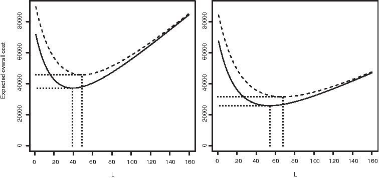
Expected overall cost as a function of L, the number of variants generated and sequenced in the randomization stage. Black curve corresponds to 100% yield and red to 80%. Left: c_primer = 8, c_fixed = 2, and c_seq = 2.8. Right: c_seq lowered to 1.5. All curves refer to NNK randomization and to a protein with M = 181 randomized positions, as in the Bacillus subtilis lipase A experiment.

It can be seen that the optimal L in the case of 100% yield is L* = 39, which correspond to an optimal expected overall cost of E[C(L*)] = 37,272. The cost curve varies considerably near its minimum: Sequencing L = 96 variants in the randomization stage (an entire microplate) would result in an expected overall cost of 54,012, an increase of 45%. As expected, the optimal overall expected cost increases when the yield drops to 80%, to 45,877, which is attained with L* = 49.

Over the past 2 decades, technological advances have kept lowering biotechnological costs considerably, and are expected to continue doing so. The right panel of Figure 1 shows how the results change when the sequencing cost c_seq drops from 2.8 to 1.5. With 100% yield, the optimal value of L is L* = 54, which correspond to an optimal expected overall cost of 25,814. Under 80% yield, the figures change to L* = 68 and E[C(L*)] = 31,522.

The influence of the yield on the expected overall cost can be seen in more detail in Figure 2. The left panel of the figure depicts the optimal value of the cost function (the minimal point of the cost curve in Figure 1) as a function of the yield. As expected, the resulting curve tends to infinity as the yield approaches zero. The influence of decreasing the yield on L* is a priori less clear, as lower yield affects adversely both stages of the scanning process. The right panel of Figure 2 shows that not only the optimal overall cost, but also L*, increases as the yield tends to 0.

OPEN IN VIEWER

FIG. 2.

Left: The optimal expected overall cost, E[C(L)], as a function of the yield. Right: The optimal number of variants generated and sequenced in the randomization stage, L*, as a function of the yield.

Although the distribution of C(L) is certainly not normal, it may be well approximated by a normal distribution having the mean and variance of C(L) (Equations (3) and (4) in the Methods section), as shown in Figure 3. The central limit theorem explains the good fit when M, the number of scanned positions, is large (M = 181 in the left panel), but the fit remains good also when only few positions are scanned (M = 10 in the right panel).

OPEN IN VIEWER

FIG. 3.

Histogram of 10,000 simulated values of C(L), the total cost of the experiment, with a density plot of a normal distribution having the mean and variance of C(L). Left: M = 181, as in the lipase A study. Right: M = 10. In both cases L = 40, and other parameters are as in the left panel of Figure 1.

All the results presented so far assumed that NNK randomization was used. Figure 4 shows the expected overall cost as a function of L for two additional randomization schemes: the “22c-trick,” and the method of Tang et al. (2012). It can be seen that in both methods, the savings due to the improved efficiency do not compensate for the increase in primer cost.

OPEN IN VIEWER

FIG. 4.

Expected overall cost as a function of L, the number of variants generated and sequenced in the randomization stage, for three randomization schemes. Left: 100% yield. Right: 80% yield. Other parameters are as in the left panel of Figure 1.

4. Discussion

The goal of this work is to establish a methodology for determining the optimal resource allocation, when scanning all single-point mutants of a protein. Only a small adjustment is needed if one wishes to scan not all 19 substitutions at each position, but rather, some other predetermined number. One can analyze similarly also a process whereby all two-mutant variants of a protein are to be systematically generated.

The cost function we employ is rather simplistic, as it ignores, for example, the cost of the nonexpendable laboratory equipment. Still, it captures the most essential components of the situation: the tradeoff between increased randomization cost and increased site-directed mutagenesis cost, as a result of varying L, the number of variants generated and sequenced in the randomization stage. Neglecting the integrality constraint, the optimal L is the solution of the equation obtained by equating the derivative of the objective function to zero. This solution lends itself to an intuitive interpretation: When increasing L by a unit, the per-position increase in the randomization cost is the derivative of the expression 2c_primer + c_fixed + Lc_seq, which is exactly c_seq, as one more variant will have to be sequenced. At the same time, the expected decrease in the site-directed mutagenesis cost (a decrease that takes place as fewer variants will have to be generated individually) is the derivative of (2c_primer + c_fixed + c_seq)E(K_a,L). The optimal L is indeed the value that makes these two forces equal to each other, and is therefore found by equating to zero the derivative of their sum, the total expected cost.

The original problem formulation assumed that the same L will be used in the randomization stage for all of the protein's position. However, since each position is dealt with separately, and since the per-position cost C_i(L) depends on the specific wild-type amino acid at that position, one could in principle find and use an optimal L for each position. By doing so the overall expected cost will indeed decrease, but it can be shown mathematically that the decrease will be of only about 1%, a small difference that will most likely get buried in the experimental noise.

Our analysis shows that the yield has a substantial influence on both the optimal cost and on the optimal L required to attain it. We recommend estimating the yield in a small preliminary experiment, and then use the estimate for determining the optimal L in the full-scale experiment.

In the process studied in this work, the genetic diversity created in the randomization stage was generated via saturation mutagenesis. Other alternatives are random mutagenesis techniques such as error-prone PCR (Cadwell and Joyce, 1992) and SeSaM (Wong et al., 2004), which have been used successfully in many mutagenesis experiments. However, upon analyzing mathematically these alternatives, it turns out that even under ideal conditions (zero probability for premature stop codons and complete control over the mutation spectrum), the resulting expected overall cost will be considerably higher than that obtained via saturation mutagenesis. The reason for this is that random mutagenesis protocols are whole-protein methods, which invariably produce a large portion of multiple-point mutants, whereas the experimental goal discussed in our work is to generate systematically only single-point mutants. The inevitable additional cost, incurred by generating and sequencing these multiple-point mutants, makes random mutagenesis methods less suitable for our specific goal. Another alternative for creating the desired library would be via a massive use of gene synthesis; however, at the current synthesis prices, this approach will be about an order of magnitude more expensive than the two-stage process studied above.