Simultaneous Folding of Alternative RNA Structures with Mutual Constraints: An Application to Next-Generation Sequencing-based RNA Structure Probing

Abstract

Recent advances in next-generation sequencing technology have significantly promoted high-throughput experimental probing of RNA secondary structures. The resulting enzymatic or chemical probing information is then incorporated into a minimum free energy folding algorithm to predict more accurate RNA secondary structures. A drawback of this approach is that it does not consider the presence of alternative RNA structures. In addition, the alternative RNA structures may contaminate experimental probing information of each other and direct the minimum free-energy folding to a wrong direction. In this article, we present a combinatorial solution for this problem, where two alternative structures can be folded simultaneously given the experimental probing information regarding the mixture of these two alternative structures. We have tested our algorithm with artificially generated mixture probing data on adenine riboswitch and thiamine pyrophosphate (TPP) riboswitch. The experimental results show that our algorithm can successfully recover the ON and OFF structures of these riboswitches.

1. Introduction

The structures of noncoding RNAs are critical in understanding the transcriptome, including structure–function relationship, stability of the RNA transcripts, and various regulations that may be applied (Eddy, 2001; Storz, 2002; Martin and Ephrussi, 2009). Recently, many enzymatic and chemical RNA structure-probing techniques have been coupled with next-generation sequencing, aiming at producing genome-wide RNA structure maps. In a high-throughput RNA structure-probing experiment, the RNA samples are treated with restriction enzymes or chemical reagents, which have preferential reactivity with helix or loop regions of the RNA transcripts. The resulting fragments of the reaction are pulled out and sequenced to recover RNA structural information (Wan et al., 2011). After sequencing, one can see discrepancies in the reads mapping profile between the paired and unpaired regions. The major idea of this technique is very similar to the traditional RNA probing techniques (Weeks, 2010), except that the resulting fragments are being sequenced using high-throughput next-generation sequencing rather than electrophoresis.

Kertesz et al. (2010) pioneered whole-genome RNA secondary structure probing and applied this novel technique to the yeast genome. Underwood et al. (2010) modified this technique with an alternative restriction enzyme and applied it to the mouse genome to discover novel ncRNAs. Besides restriction enzymes, chemicals have also been used as probing reagents. A technique named SHAPE uses chemical reagents such as NMIA or 1M7 to preferentially react with single-stranded RNA transcripts (Merino et al., 2005; Wilkinson et al., 2006; Mortimer and Weeks, 2007). Later, SHAPE technique was coupled with next-generation sequencing (SHAPE-seq) by Lucks et al. (2011) to improve its throughput and application. Although not yet applied to genome-wide analysis, SHAPE-seq has demonstrated its strong potential by accurately recovering the secondary structures of 16S and 23S ribosomal RNAs (Deigan et al., 2009).

The resulting output of these techniques is the potential for each site of the RNA transcript to react with the probing enzyme or reagent. The potential, also termed reactivity, is usually derived from the read mappings (normalized with a control experiment) of the chemical probing experiment (Aviran et al., 2011). Take the SHAPE experiment, for example, a site with reactivity ‘1’ indicates that it is highly reactive to the chemical reagent, suggesting a free (unpaired) configuration of the site. On the other hand, a site with reactivity ‘0’ indicates a restricted (paired) configuration of the site. These site-wise reactivities are usually transformed into pseudoenergies and incorporated into the existing minimum free energy (MFE) folding tools, such as RNAstructure (Reuter and Mathews, 2010), to predict the structure of the RNA transcript (Deigan et al., 2009; Low and Weeks, 2010). Recently, Washietl et al. (2012) developed an iterative approach to compute the optimal weight for the pseudoenergy that should be taken into account.

However, none of these approaches considers the presence of alternative RNA structures from the same RNA transcript (such as riboswitch elements). If alternative RNA structures are present, the reactivities for the mixture of RNA structures are generated from the experiment (Fig. 1). Such mixture reactivities may fail to capture the structural information from one, or even both, alternative RNA structures and can lead to misprediction while using current available approaches. Even though combining the experimental pseudoenergy and McCaskill's (1990) algorithm, a complete folding landscape of the RNA of interest can be generated, it is very difficult to obtain the two alternative structures of interest from an exponentially large search space (Wuchty et al., 1999; Li and Zhang, 2011). In this case, developing a new computational approach to partition the mixture of reads and explicitly predict the two alternative structures of interest is extremely important for extending experimental RNA structure-probing applications.

FIG. 1.

An overview of the RNA mutually constrained folding problem. A set of mixture of reactivities is generated as the enzymatic/chemical probing information of two alternative structures from the same RNA sequence. Assume the probing enzymes/chemical reagents will preferentially attack the unpaired (loop) regions (the blue arrows) of the RNA structures. High reactivities are expected to be observed at these regions, while low reactivities are expected for the paired regions. With the presence of both alternative structures (assuming the partition is 50%–50%), their individual reactivities are attenuated by each other. Finally, a mixture of reactivities of both alternative structures are observed from the experiment. The problem we aim to solve is how to infer both alternative structures from the mixture of reactivities.

We propose considering the observed reactivity as a mixture before performing the constrained folding algorithm. Ideally, if the correct assignment of the reactivities is given, we can perform the traditional constrained folding using the two sets of reactivities separately and reach satisfying results. However, unlike the reads assignment problems, there is no sequence discrepancy between these two RNA transcripts. Therefore, its very difficult to devise a statistical framework to infer the real partition. Thus, we will simultaneously fold these two alternative structures, such that (1) the sum of their free energies is minimized, and (2) the discrepancy between the expected and the observed reactivity profiles is minimized (Fig. 1).

We refer to this problem as the RNA mutually constrained folding problem, because each of the two alternative structures may exert constraint on, or be constrained by, the other structure. Therefore, to solve the RNA mutually constrained folding problem, we devise a combinatorial algorithm that finds the optimal solution by enumerating all possible constraining structures and constraining orders (which will be formally defined in the Methods section). We first present an algorithm using the Nussinov's energy model (Nussinov et al., 1978) (base-pair maximization). The algorithm can be run within O(l⁸) time and O(l⁵) space, where l is the length of the RNA sequence. To make the algorithm more applicable in real cases, we further present an improved algorithm that is guided by stacks (continuously nested base pairs), with the implementation of Turner's energy model (free-energy minimization). The improved algorithm can run within O(n⁵) time and O(n³l) space, where n is the number of stacks and n < l in most real scenarios (Bafna et al., 2006). In this case, we can significantly reduce the running time and space consumption, and the algorithm can be applied to predict alternative structures of real RNA sequences.

We implemented the improved algorithm into a program called MutualFold using GNU C++. Using artificially generated reactivities on adenine and thiamine pyrophosphate (TPP) riboswitches, we showed that our program, MutualFold, can successfully recover the major scaffold of the true alternative structures given a set of mixture reactivities. On the contrary, the traditional energy minimization approach, both with and without reactivity as an auxiliary information, failed to predict one or both of the alternative structures. In this case, we anticipate that the proposed MutualFold algorithm will significantly promote future RNA alternative structure prediction and related research.

2. Methods

In this section, we will introduce the RNA mutually constrained folding problem, which predicts two alternative RNA structures of the minimum sum of free energies with the consideration of step-wise folding constraint effect. We will first present the basic problem formulation in section 2.1, and then present a straightforward solution to the problem using Nussinov's energy model in section 2.2. We will further introduce a more realistic algorithm with sophisticated Turner's energy model and an improved time complexity in section 2.3. Finally, we will discuss how we handle reactivities and pseudoenergies in section 2.4.

2.1. Problem formulation

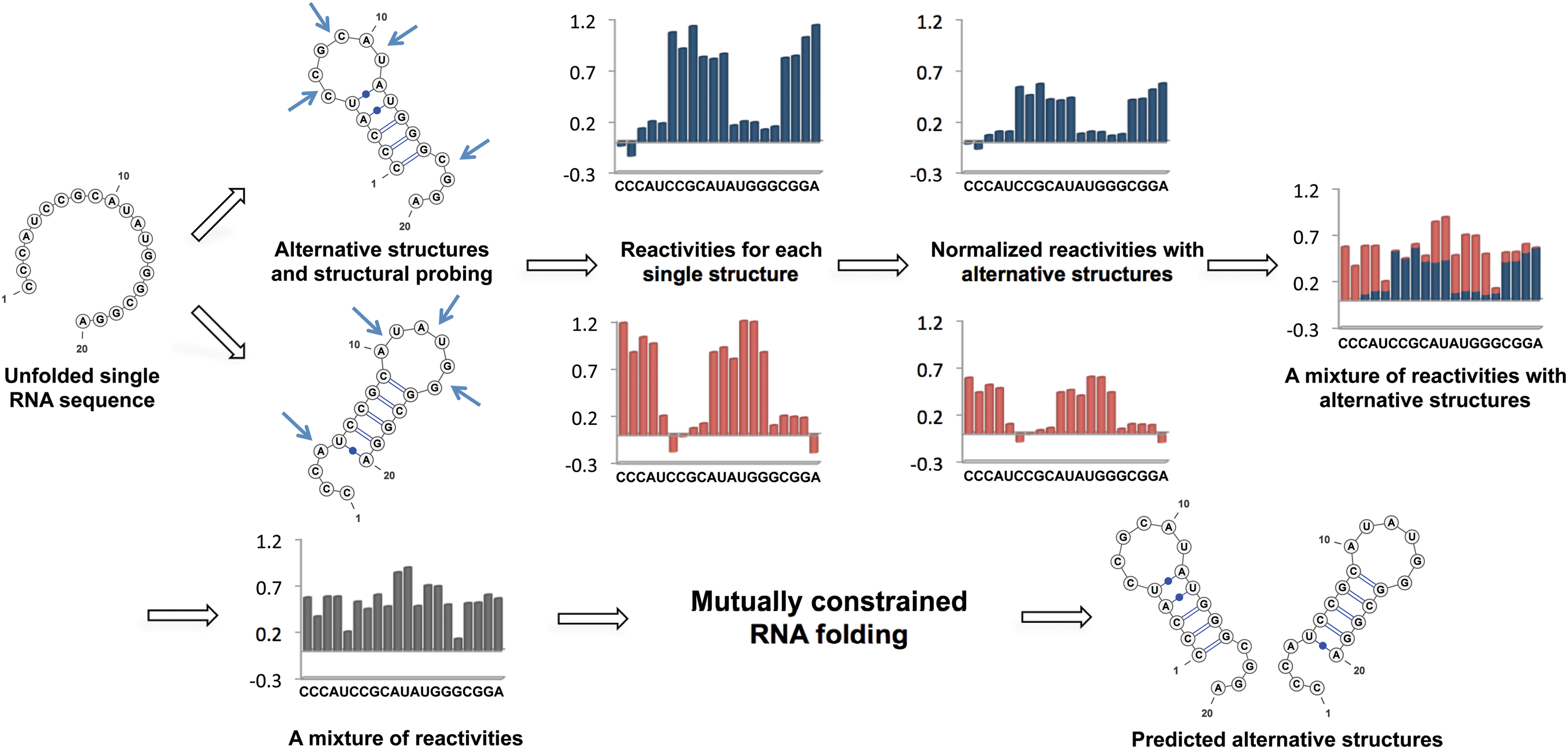
We begin the formulation of the RNA mutually constrained folding problem by introducing the inputs of the algorithm. The algorithm requires three inputs: (1) the RNA sequence S with length l, from which the alternative structures are to be predicted; (2) a set of observed mixture reactivities \documentclass{aastex}\usepackage{amsbsy}\usepackage{amsfonts}\usepackage{amssymb}\usepackage{bm}\usepackage{mathrsfs}\usepackage{pifont}\usepackage{stmaryrd}\usepackage{textcomp}\usepackage{portland, xspace}\usepackage{amsmath, amsxtra}\pagestyle{empty}\DeclareMathSizes{10}{9}{7}{6}\begin{document} $$R = \{r_0 , r_1 , \ldots , r_{l - 1} \}$$ \end{document} , where r_i is the reactivity for the ith nucleotide; and (3) the expected partition of these two alternative structures ψ, where 0 ≤ ψ ≤ 1.

The outputs of the algorithm are two simultaneously predicted RNA structures T^A and T^B. We expect that the predicted structures are thermodynamically stable, or, the sum of the real free energies of the two structures, say E^⋅(T^A) + E^⋅(T^B) (a solid dot is used to indicate real energy), is minimized. At the same time, we also expect that the discrepancy between the expected and the observed reactivity profile, say |R−mixture(R(T^A), R(T^B))|, is minimized. Here, R(T^A) refers to the expected reactivity profile of structure T^A alone. The discrepancy of the reactivity profiles is usually quantified by the pseudoenergy (Deigan et al., 2009; Low and Weeks, 2010), and we adopt this measurement as well. For example, let T^A(i) be the structural configuration of the ith nucleotide in T^A, and assume T^A(i) is paired. If the probing enzyme/chemical reagent is not reactive to the paired nucleotides, we should expect rather low reactivity observed at this nucleotide, that is, \documentclass{aastex}\usepackage{amsbsy}\usepackage{amsfonts}\usepackage{amssymb}\usepackage{bm}\usepackage{mathrsfs}\usepackage{pifont}\usepackage{stmaryrd}\usepackage{textcomp}\usepackage{portland, xspace}\usepackage{amsmath, amsxtra}\pagestyle{empty}\DeclareMathSizes{10}{9}{7}{6}\begin{document} $$\hat{r}_i = 0$$ \end{document} . The following formula (reformulated from Deigan et al., 2009 and Low and Weeks, 2010) has been proposed to compute the pseudoenergy E^∘ (a void dot is used to indicate pseudoenergy): \documentclass{aastex}\usepackage{amsbsy}\usepackage{amsfonts}\usepackage{amssymb}\usepackage{bm}\usepackage{mathrsfs}\usepackage{pifont}\usepackage{stmaryrd}\usepackage{textcomp}\usepackage{portland, xspace}\usepackage{amsmath, amsxtra}\pagestyle{empty}\DeclareMathSizes{10}{9}{7}{6}\begin{document} \begin{align*}E^{\circ} (\mid r_i - \hat{r}_i \mid) = m * \log (\mid r_i - \hat{r}_i \mid + 1) + b , \tag{1}\end{align*} \end{document}

where m is positive and b is a negative constant. If \documentclass{aastex}\usepackage{amsbsy}\usepackage{amsfonts}\usepackage{amssymb}\usepackage{bm}\usepackage{mathrsfs}\usepackage{pifont}\usepackage{stmaryrd}\usepackage{textcomp}\usepackage{portland, xspace}\usepackage{amsmath, amsxtra}\pagestyle{empty}\DeclareMathSizes{10}{9}{7}{6}\begin{document} $$\mid r_i - \hat{r}_i \mid = 0$$ \end{document} (i.e., no discrepancy), \documentclass{aastex}\usepackage{amsbsy}\usepackage{amsfonts}\usepackage{amssymb}\usepackage{bm}\usepackage{mathrsfs}\usepackage{pifont}\usepackage{stmaryrd}\usepackage{textcomp}\usepackage{portland, xspace}\usepackage{amsmath, amsxtra}\pagestyle{empty}\DeclareMathSizes{10}{9}{7}{6}\begin{document} $$E^{\circ} (\mid r_i - \hat{r}_i \mid) = b$$ \end{document} , and a favorable pseudoenergy is returned to indicate that the assumption of T^A(i) being paired is correct. If \documentclass{aastex}\usepackage{amsbsy}\usepackage{amsfonts}\usepackage{amssymb}\usepackage{bm}\usepackage{mathrsfs}\usepackage{pifont}\usepackage{stmaryrd}\usepackage{textcomp}\usepackage{portland, xspace}\usepackage{amsmath, amsxtra}\pagestyle{empty}\DeclareMathSizes{10}{9}{7}{6}\begin{document} $$\mid r_i - \hat{r}_i \mid > 0 , E^{\circ} (\mid r_i - \hat{r}_i \mid) > b$$ \end{document} , and a less favorable pseudoenergy is returned to question the assumption. We can simplify the notation of pseudoenergy as E^∘(r_i) since \documentclass{aastex}\usepackage{amsbsy}\usepackage{amsfonts}\usepackage{amssymb}\usepackage{bm}\usepackage{mathrsfs}\usepackage{pifont}\usepackage{stmaryrd}\usepackage{textcomp}\usepackage{portland, xspace}\usepackage{amsmath, amsxtra}\pagestyle{empty}\DeclareMathSizes{10}{9}{7}{6}\begin{document} $$\hat{r}$$ \end{document} is known. We also assume the pseudoenergies to be additive as the real energies, that is, \documentclass{aastex}\usepackage{amsbsy}\usepackage{amsfonts}\usepackage{amssymb}\usepackage{bm}\usepackage{mathrsfs}\usepackage{pifont}\usepackage{stmaryrd}\usepackage{textcomp}\usepackage{portland, xspace}\usepackage{amsmath, amsxtra}\pagestyle{empty}\DeclareMathSizes{10}{9}{7}{6}\begin{document} $$E^{\circ} (T_{i , j}) = \sum^j_{k = i}E^{\circ} (r_k)$$ \end{document} . In this case, the pseudo energy can be incorporated into the real free energy, that is, E(T^A) = E^⋅(T^A) + E^∘(T^A), and our algorithm will minimize E(T^A) + E(T^B) to simultaneously consider thermodynamic stability and reactivity discrepancy. Now, we can formally define the RNA mutually constrained folding problem as follows:

Input: an RNA sequence S, a set of mixture reactivities R, and an expected partition ψ.

Output: two RNA structures T^A and T^B of S, such that the sum of free energies (including both real and pseudo energies) E(T^A) + E(T^B) is minimized.

The key to the solution of this problem is based on the understanding of how T^A and T^B are mutually constrained, that is, how the folding of one structure may exert constraint on, or be constrained by, the other structure. Recall that r_i is the observed reactivity at the ith nucleotide, and let it be a mixture (with a ratio ψ) of the reactivity from structure A (defined as \documentclass{aastex}\usepackage{amsbsy}\usepackage{amsfonts}\usepackage{amssymb}\usepackage{bm}\usepackage{mathrsfs}\usepackage{pifont}\usepackage{stmaryrd}\usepackage{textcomp}\usepackage{portland, xspace}\usepackage{amsmath, amsxtra}\pagestyle{empty}\DeclareMathSizes{10}{9}{7}{6}\begin{document} $$r_i^A$$ \end{document} ) and structure B (defined as \documentclass{aastex}\usepackage{amsbsy}\usepackage{amsfonts}\usepackage{amssymb}\usepackage{bm}\usepackage{mathrsfs}\usepackage{pifont}\usepackage{stmaryrd}\usepackage{textcomp}\usepackage{portland, xspace}\usepackage{amsmath, amsxtra}\pagestyle{empty}\DeclareMathSizes{10}{9}{7}{6}\begin{document} $$r_i^B$$ \end{document} ). In other words, \documentclass{aastex}\usepackage{amsbsy}\usepackage{amsfonts}\usepackage{amssymb}\usepackage{bm}\usepackage{mathrsfs}\usepackage{pifont}\usepackage{stmaryrd}\usepackage{textcomp}\usepackage{portland, xspace}\usepackage{amsmath, amsxtra}\pagestyle{empty}\DeclareMathSizes{10}{9}{7}{6}\begin{document} $$r_i = f (\psi , r_i^A , r_i^B)$$ \end{document} . Also assume that we can represent the observed reactivity \documentclass{aastex}\usepackage{amsbsy}\usepackage{amsfonts}\usepackage{amssymb}\usepackage{bm}\usepackage{mathrsfs}\usepackage{pifont}\usepackage{stmaryrd}\usepackage{textcomp}\usepackage{portland, xspace}\usepackage{amsmath, amsxtra}\pagestyle{empty}\DeclareMathSizes{10}{9}{7}{6}\begin{document} $$r_i^B$$ \end{document} by its expectation \documentclass{aastex}\usepackage{amsbsy}\usepackage{amsfonts}\usepackage{amssymb}\usepackage{bm}\usepackage{mathrsfs}\usepackage{pifont}\usepackage{stmaryrd}\usepackage{textcomp}\usepackage{portland, xspace}\usepackage{amsmath, amsxtra}\pagestyle{empty}\DeclareMathSizes{10}{9}{7}{6}\begin{document} $$\hat{r}_i^B$$ \end{document} , which is determined by the structural configuration T^B(i), i.e., \documentclass{aastex}\usepackage{amsbsy}\usepackage{amsfonts}\usepackage{amssymb}\usepackage{bm}\usepackage{mathrsfs}\usepackage{pifont}\usepackage{stmaryrd}\usepackage{textcomp}\usepackage{portland, xspace}\usepackage{amsmath, amsxtra}\pagestyle{empty}\DeclareMathSizes{10}{9}{7}{6}\begin{document} $$r_i^B = \hat{r}_i^B = g (T^B (i))$$ \end{document} . Therefore, \documentclass{aastex}\usepackage{amsbsy}\usepackage{amsfonts}\usepackage{amssymb}\usepackage{bm}\usepackage{mathrsfs}\usepackage{pifont}\usepackage{stmaryrd}\usepackage{textcomp}\usepackage{portland, xspace}\usepackage{amsmath, amsxtra}\pagestyle{empty}\DeclareMathSizes{10}{9}{7}{6}\begin{document} $$r_i = f_g (\psi , r_i^A , T^B (i))$$ \end{document} and finally, \documentclass{aastex}\usepackage{amsbsy}\usepackage{amsfonts}\usepackage{amssymb}\usepackage{bm}\usepackage{mathrsfs}\usepackage{pifont}\usepackage{stmaryrd}\usepackage{textcomp}\usepackage{portland, xspace}\usepackage{amsmath, amsxtra}\pagestyle{empty}\DeclareMathSizes{10}{9}{7}{6}\begin{document} $$r_i^A = f^{\prime}_g (\psi , r_i , T^B (i))$$ \end{document} . For the sake of simplicity, we will write \documentclass{aastex}\usepackage{amsbsy}\usepackage{amsfonts}\usepackage{amssymb}\usepackage{bm}\usepackage{mathrsfs}\usepackage{pifont}\usepackage{stmaryrd}\usepackage{textcomp}\usepackage{portland, xspace}\usepackage{amsmath, amsxtra}\pagestyle{empty}\DeclareMathSizes{10}{9}{7}{6}\begin{document} $$r_i^A = f (T^B (i))$$ \end{document} , as ψ and r_i are not variables and are given as the inputs. In this case, the pseudoenergy used for folding T^A is affected by the structure of T^B and vise versa. In this case, T^A and T^B are mutually constrained.

With the understanding of mutual constraints, we can easily devise a brute force solution, which takes exponential time. We can enumerate all possible T^B as constraints and fold T^A correspondingly. The pair of T^A and T^B that results in the minimum sum of free energies can be taken as the optimal solution. However, this approach is computationally expensive, as there are an exponential number of possible structures that are to be enumerated as the structural constraint T^B. To resolve this issue, we can break down the problem into smaller subproblems using dynamic programming formulation. Let \documentclass{aastex}\usepackage{amsbsy}\usepackage{amsfonts}\usepackage{amssymb}\usepackage{bm}\usepackage{mathrsfs}\usepackage{pifont}\usepackage{stmaryrd}\usepackage{textcomp}\usepackage{portland, xspace}\usepackage{amsmath, amsxtra}\pagestyle{empty}\DeclareMathSizes{10}{9}{7}{6}\begin{document} $$(i_1 \ldots j_1) ^A$$ \end{document} be a substructure in T^A (which begins with S_i₁ and ends with S_j₁), and \documentclass{aastex}\usepackage{amsbsy}\usepackage{amsfonts}\usepackage{amssymb}\usepackage{bm}\usepackage{mathrsfs}\usepackage{pifont}\usepackage{stmaryrd}\usepackage{textcomp}\usepackage{portland, xspace}\usepackage{amsmath, amsxtra}\pagestyle{empty}\DeclareMathSizes{10}{9}{7}{6}\begin{document} $$(i_2 \ldots j_2) ^B$$ \end{document} be a substructure in T^B (which begins with S_i₂ and ends with S_j₂). These two substructures may or may not overlap each other. If the optimal structures (with the minimum sum of energies) adopted by both subregions, say T_i_1,j1;i2,j2, are known, we can use them as structural constraints to fold nearby RNA sequences. We can reach the final solution using this approach by extending i₁, j₁ to 0 and i₂, j₂ to l−1.

To guarantee optimality, we need to consider all possible constraining orders when computing T_i_1,j1;i2,j2. For example, let “−” indicate a void region that exerts no structural constraint, T_{−,−;i2,k2} → T_i_1,j1;i2,k2 → T_i_1,j1;i2,j2 (where i₂ ≤ k₂ ≤ j₂) represents the following constraining order: (1) \documentclass{aastex}\usepackage{amsbsy}\usepackage{amsfonts}\usepackage{amssymb}\usepackage{bm}\usepackage{mathrsfs}\usepackage{pifont}\usepackage{stmaryrd}\usepackage{textcomp}\usepackage{portland, xspace}\usepackage{amsmath, amsxtra}\pagestyle{empty}\DeclareMathSizes{10}{9}{7}{6}\begin{document} $$(i_2 \ldots k_2) ^B$$ \end{document} is folded without constraint, (2) \documentclass{aastex}\usepackage{amsbsy}\usepackage{amsfonts}\usepackage{amssymb}\usepackage{bm}\usepackage{mathrsfs}\usepackage{pifont}\usepackage{stmaryrd}\usepackage{textcomp}\usepackage{portland, xspace}\usepackage{amsmath, amsxtra}\pagestyle{empty}\DeclareMathSizes{10}{9}{7}{6}\begin{document} $$(i_1 \ldots j_1) ^A$$ \end{document} is folded by applying \documentclass{aastex}\usepackage{amsbsy}\usepackage{amsfonts}\usepackage{amssymb}\usepackage{bm}\usepackage{mathrsfs}\usepackage{pifont}\usepackage{stmaryrd}\usepackage{textcomp}\usepackage{portland, xspace}\usepackage{amsmath, amsxtra}\pagestyle{empty}\DeclareMathSizes{10}{9}{7}{6}\begin{document} $$(i_2 \ldots k_2) ^B$$ \end{document} as a structural constraint, and (3) \documentclass{aastex}\usepackage{amsbsy}\usepackage{amsfonts}\usepackage{amssymb}\usepackage{bm}\usepackage{mathrsfs}\usepackage{pifont}\usepackage{stmaryrd}\usepackage{textcomp}\usepackage{portland, xspace}\usepackage{amsmath, amsxtra}\pagestyle{empty}\DeclareMathSizes{10}{9}{7}{6}\begin{document} $$(k_2 + 1 \ldots j_2) ^B$$ \end{document} is folded by applying \documentclass{aastex}\usepackage{amsbsy}\usepackage{amsfonts}\usepackage{amssymb}\usepackage{bm}\usepackage{mathrsfs}\usepackage{pifont}\usepackage{stmaryrd}\usepackage{textcomp}\usepackage{portland, xspace}\usepackage{amsmath, amsxtra}\pagestyle{empty}\DeclareMathSizes{10}{9}{7}{6}\begin{document} $$(i_1 \ldots j_1) ^A$$ \end{document} as a structural constraint. Other constraining orders are possible as well. For example, T_{−,−;i2,k2} → T_i_1,k1;i2,k2 → T_i_1,k1;i2,j2 → T_i_1,j1;i2,j2 (where i₁ ≤ k₁ ≤ j₁) can act as an alternative constraining order to be traversed during the computation of T_i_1,j1;i2,j2. In summary, all subregions (T_i_1,j1;i2,j2) and all constraining orders need to be taken into account in the algorithm. We present a combinatorial solution using the Nussinov's energy model (Nussinov et al., 1978) in the following section.

2.2. An algorithm with Nussinov's energy model

In this section, we will introduce a solution for the RNA mutually constrained folding problem using Nussinov's energy model (Nussinov et al., 1978) to facilitate the understanding of the major idea. The object function of Nussinov's RNA folding formulation is to maximize the number of base pairs, instead of minimizing the free energy, of the predicted RNA structure. Therefore, denote F(i₁,j₁;i₂,j₂) as the maximum number of base pairs within the subregions \documentclass{aastex}\usepackage{amsbsy}\usepackage{amsfonts}\usepackage{amssymb}\usepackage{bm}\usepackage{mathrsfs}\usepackage{pifont}\usepackage{stmaryrd}\usepackage{textcomp}\usepackage{portland, xspace}\usepackage{amsmath, amsxtra}\pagestyle{empty}\DeclareMathSizes{10}{9}{7}{6}\begin{document} $$(i_1 \ldots j_1) ^A$$ \end{document} and \documentclass{aastex}\usepackage{amsbsy}\usepackage{amsfonts}\usepackage{amssymb}\usepackage{bm}\usepackage{mathrsfs}\usepackage{pifont}\usepackage{stmaryrd}\usepackage{textcomp}\usepackage{portland, xspace}\usepackage{amsmath, amsxtra}\pagestyle{empty}\DeclareMathSizes{10}{9}{7}{6}\begin{document} $$(i_2 \ldots j_2) ^B$$ \end{document} , where \documentclass{aastex}\usepackage{amsbsy}\usepackage{amsfonts}\usepackage{amssymb}\usepackage{bm}\usepackage{mathrsfs}\usepackage{pifont}\usepackage{stmaryrd}\usepackage{textcomp}\usepackage{portland, xspace}\usepackage{amsmath, amsxtra}\pagestyle{empty}\DeclareMathSizes{10}{9}{7}{6}\begin{document} $$F (i_1 , j_1; i_2 , j_2) = F (T_{i_1 , j_1; i_2 , j_2}^A) + F (T_{i_1 , j_1; i_2 , j_2}^B)$$ \end{document} , and \documentclass{aastex}\usepackage{amsbsy}\usepackage{amsfonts}\usepackage{amssymb}\usepackage{bm}\usepackage{mathrsfs}\usepackage{pifont}\usepackage{stmaryrd}\usepackage{textcomp}\usepackage{portland, xspace}\usepackage{amsmath, amsxtra}\pagestyle{empty}\DeclareMathSizes{10}{9}{7}{6}\begin{document} $$T_{i_1 , j_1; i_2 , j_2}^A$$ \end{document} is the structure for the subregion \documentclass{aastex}\usepackage{amsbsy}\usepackage{amsfonts}\usepackage{amssymb}\usepackage{bm}\usepackage{mathrsfs}\usepackage{pifont}\usepackage{stmaryrd}\usepackage{textcomp}\usepackage{portland, xspace}\usepackage{amsmath, amsxtra}\pagestyle{empty}\DeclareMathSizes{10}{9}{7}{6}\begin{document} $$(i_1 \ldots j_1) ^A$$ \end{document} of T_i_1,j2;i2,j2. Note that F also contains both real and pseudo base pairs, that is, F = F^⋅ + F^∘. Also denote \documentclass{aastex}\usepackage{amsbsy}\usepackage{amsfonts}\usepackage{amssymb}\usepackage{bm}\usepackage{mathrsfs}\usepackage{pifont}\usepackage{stmaryrd}\usepackage{textcomp}\usepackage{portland, xspace}\usepackage{amsmath, amsxtra}\pagestyle{empty}\DeclareMathSizes{10}{9}{7}{6}\begin{document} $$F^A (i_1 , j_1 , T_{i_2 , j_2}^B)$$ \end{document} as the maximal number of base pairs within the subregions \documentclass{aastex}\usepackage{amsbsy}\usepackage{amsfonts}\usepackage{amssymb}\usepackage{bm}\usepackage{mathrsfs}\usepackage{pifont}\usepackage{stmaryrd}\usepackage{textcomp}\usepackage{portland, xspace}\usepackage{amsmath, amsxtra}\pagestyle{empty}\DeclareMathSizes{10}{9}{7}{6}\begin{document} $$(i_1 \ldots j_1) ^A$$ \end{document} given the structure \documentclass{aastex}\usepackage{amsbsy}\usepackage{amsfonts}\usepackage{amssymb}\usepackage{bm}\usepackage{mathrsfs}\usepackage{pifont}\usepackage{stmaryrd}\usepackage{textcomp}\usepackage{portland, xspace}\usepackage{amsmath, amsxtra}\pagestyle{empty}\DeclareMathSizes{10}{9}{7}{6}\begin{document} $$T_{i_2 , j_2}^B$$ \end{document} as a structural constraint. For the sake of clarity, we underline the terms that correspond to the terminal cases, whose values can be directly computed or looked up. We can compute F(i₁,j₁;i₂,j₂) using the following recursive function: \documentclass{aastex}\usepackage{amsbsy}\usepackage{amsfonts}\usepackage{amssymb}\usepackage{bm}\usepackage{mathrsfs}\usepackage{pifont}\usepackage{stmaryrd}\usepackage{textcomp}\usepackage{portland, xspace}\usepackage{amsmath, amsxtra}\pagestyle{empty}\DeclareMathSizes{10}{9}{7}{6}\begin{document} \begin{align*} & F (i_1 , j_1; i_2 , j_2) \\& = \max \begin{cases}0 \quad [ {\rm if} \ i_1 = j_1 \ {\rm and} \ i_2 = j_2 ] , \\ F (i_1 + 1 , j_1 \,- \, 1; i_2 , j_2) \, + \, 1 \, + \, \underline{F^{\circ}} (f (T_{i_1 + 1 , j_1 - 1; i_2 , j_2}^B (i_1))) + \underline{F^{\circ}} (f (T_{i_1 + 1 , j_1 - 1; i_2 , j_2}^B (j_1))) [{\rm if} \ i_1 \ pairs with \ j_1 ] , \\ F (i_1 , j_1; i_2 + 1 , j_2 - 1) \, + \, 1 \, +\, \underline{F^{\circ}} (f (T_{i_1 , j_1; i_2 + 1 , j_2 - 1}^A (i_2))) + \underline{F^{\circ}} (f (T_{i_1 , j_1; i_2 + 1 , j_2 - 1}^A (j_2))) [{\rm if} \ i_2 \ {pairs with} \ j_2 ] , \\ \max_{i_1 < k_1 \leq j_1} \{F (k_1 + 1 , j_1; i_2 , j_2) + F^A (i_1 , k_1 , T_{{k_1 + 1 , j_1; i_2 , j_2}}^B) \} , \\ \max_{i_1 \leq k_1 < j_1} \{F (i_1 , k_1 - 1; i_2 , j_2) + F^A (k_1 , j_1 , T_{{i_1 , k_1 - 1; i_2 , j_2}}^B) \} , \\ \max_{i_2 < k_2 \leq j_2} \{F (i_1 , j_1; k_2 + 1 , j_2) + F^B (i_2 , k_2 , T_{{i_1 , j_1; k_2 + 1 , j_2}}^A) \} , \\ \max_{i_2 \leq k_2 < j_2} \{F (i_1 , j_1; i_2 , k_2 - 1) + F^B (k_2 , j_2 , T^A_{i_1 , j_1; i_2 , k_2 - 1}) \}. \end{cases} \tag{2} \end{align*} \end{document}

The first case described in Equation (2) corresponds to a boundary case where no base pair is formed. The second and third cases correspond to paired cases, where the outmost nucleotides (i₁ and j₁, or i₂ and j₂, respectively) form a base pair. In this case, “1” is added to indicate the base pair that has formed, and how well the observed reactivity supports the pair is evaluated by pseudo base pairs ( F ^∘ s). The last four cases try all possible branching points with different constraining orders. Take the fourth case as an example; the last added structural component (i.e., \documentclass{aastex}\usepackage{amsbsy}\usepackage{amsfonts}\usepackage{amssymb}\usepackage{bm}\usepackage{mathrsfs}\usepackage{pifont}\usepackage{stmaryrd}\usepackage{textcomp}\usepackage{portland, xspace}\usepackage{amsmath, amsxtra}\pagestyle{empty}\DeclareMathSizes{10}{9}{7}{6}\begin{document} $$(i_1 \ldots k_1) ^A$$ \end{document} ) will be predicted using the existing optimal substructure (i.e., \documentclass{aastex}\usepackage{amsbsy}\usepackage{amsfonts}\usepackage{amssymb}\usepackage{bm}\usepackage{mathrsfs}\usepackage{pifont}\usepackage{stmaryrd}\usepackage{textcomp}\usepackage{portland, xspace}\usepackage{amsmath, amsxtra}\pagestyle{empty}\DeclareMathSizes{10}{9}{7}{6}\begin{document} $$T_{{k_1 + 1 , j_1; i_2 , j_2}}^B$$ \end{document} ) as a constraint by the traditional Nussinov's folding algorithm (Nussinov et al., 1978) with soft constraints.

The optimal structural configuration for a region with a structural constraint, for example, \documentclass{aastex}\usepackage{amsbsy}\usepackage{amsfonts}\usepackage{amssymb}\usepackage{bm}\usepackage{mathrsfs}\usepackage{pifont}\usepackage{stmaryrd}\usepackage{textcomp}\usepackage{portland, xspace}\usepackage{amsmath, amsxtra}\pagestyle{empty}\DeclareMathSizes{10}{9}{7}{6}\begin{document} $$F^A (i , j , T_{{i_1 , j_1; i_2 , j_2}}^B)$$ \end{document} [similar for \documentclass{aastex}\usepackage{amsbsy}\usepackage{amsfonts}\usepackage{amssymb}\usepackage{bm}\usepackage{mathrsfs}\usepackage{pifont}\usepackage{stmaryrd}\usepackage{textcomp}\usepackage{portland, xspace}\usepackage{amsmath, amsxtra}\pagestyle{empty}\DeclareMathSizes{10}{9}{7}{6}\begin{document} $$F^B (i , j , T_{{i_1 , j_1; i_2 , j_2}}^A)$$ \end{document} ], can be computed as follows: \documentclass{aastex}\usepackage{amsbsy}\usepackage{amsfonts}\usepackage{amssymb}\usepackage{bm}\usepackage{mathrsfs}\usepackage{pifont}\usepackage{stmaryrd}\usepackage{textcomp}\usepackage{portland, xspace}\usepackage{amsmath, amsxtra}\pagestyle{empty}\DeclareMathSizes{10}{9}{7}{6}\begin{document} \begin{align*} & F^A (i , j , T_{{i_1 , j_1; i_2 , j_2}}^B) \\ & = \max \begin{cases}0 \quad\quad [ {\rm if} \ i = j ] , \\ F^A (i + 1 , j - 1 , T_{{i_1 , j_1; i_2 , j_2}}^B) + 1 + \underline{F^{\circ}} (f (T_{{i_1 , j_1; i_2 , j_2}}^B (i))) + \underline{F^{\circ}} (f (T_{{i_1 , j_1; i_2 , j_2}}^B (j))) \quad [ {\rm if} \ i \ {pairs with} \ j ] , \\ \max_{i < k \leq j} \{F^A (i , k - 1 , T_{{i_1 , j_1; i_2 , j_2}}^B) + F^A (k , j , T_{i_1 , j_1; i_2 , j_2}^B) \} , \end{cases} & (3) \end{align*} \end{document}

A direct implementation of this algorithm leads to an O(l⁸) time complexity and O(l⁵) space complexity. Indeed, to complete the algorithm, we need to fill up a four-dimensional dynamic programming table F, which requires O(l⁴) time. For each entry in F, O(l) time is used for traversing all branching k₁ and k₂, and O(l³) is used to compute the constrained folding F^A and F^B. Therefore, the overall time complexity would be O(l⁸). The space complexity is O(l⁵). Note that the algorithm needs to maintain the four-dimensional table F, in addition, and O(l) space is also required for each entry of F to record the corresponding optimal structure that would be used as a structural constraint in the future folding steps. Hence the overall space complexity is O(l⁵).

2.3. An improved algorithm with Turner's energy model

The time and space complexity of the previous algorithm are prohibitively high and are not feasible for most real RNA sequences. Therefore, we need to devise a more efficient algorithm. At the same time, we need to consider the more realistic Turner's energy model (Turner et al., 1988). Inspired by the idea of RNAscf (Bafna et al., 2006), we observe that the major scaffolds of RNA secondary structures can be represented by stacks. A stack, built from a number of continuously nested base pairs, form the regular A-form helix of the RNA structure that stabilizes the structure. Note that we only consider the significant stacks, that is, those with more than four base pairs and eight hydrogen bonds, as the number of these significant stacks is usually small and less than the length of the RNA sequence (Bafna et al., 2006). Therefore, at each folding step we will add a stack or a structural component enclosed by a stack. Thus we can achieve significant speedup compared to the previous algorithm with base-pair resolution.

We begin the exposition of the algorithm by introducing basic definitions of stacks and their relationships. An RNA structure can be represented by a set of significant stacks; denote the set as \documentclass{aastex}\usepackage{amsbsy}\usepackage{amsfonts}\usepackage{amssymb}\usepackage{bm}\usepackage{mathrsfs}\usepackage{pifont}\usepackage{stmaryrd}\usepackage{textcomp}\usepackage{portland, xspace}\usepackage{amsmath, amsxtra}\pagestyle{empty}\DeclareMathSizes{10}{9}{7}{6}\begin{document} $${\cal P}$$ \end{document} . A stack p can be uniquely determined by three indices: the leftmost endpoint l(p), the rightmost endpoint r(p), and the width of the stack w(p). The nucleotides at l(p) and r(p) form the outmost (smallest 5′ and largest 3′ indices) base pair of p, while l(p) + w(p) − 1 and r(p) − w(p) + 1 form the innermost base pair of p. To simplify the notations, we also say that l_I(p) and r_I(p) form the innermost base pair of p. The stacks can be partially ordered by increasing rightmost endpoints and decreasing leftmost endpoints. With such partial ordering, we can denote the ith stack in \documentclass{aastex}\usepackage{amsbsy}\usepackage{amsfonts}\usepackage{amssymb}\usepackage{bm}\usepackage{mathrsfs}\usepackage{pifont}\usepackage{stmaryrd}\usepackage{textcomp}\usepackage{portland, xspace}\usepackage{amsmath, amsxtra}\pagestyle{empty}\DeclareMathSizes{10}{9}{7}{6}\begin{document} $${\cal P}$$ \end{document} as p_i.

Let p_i and p_j be two stacks in \documentclass{aastex}\usepackage{amsbsy}\usepackage{amsfonts}\usepackage{amssymb}\usepackage{bm}\usepackage{mathrsfs}\usepackage{pifont}\usepackage{stmaryrd}\usepackage{textcomp}\usepackage{portland, xspace}\usepackage{amsmath, amsxtra}\pagestyle{empty}\DeclareMathSizes{10}{9}{7}{6}\begin{document} $${\cal P}$$ \end{document} and assume that i < j. If p_i is enclosed by p_j, that is, l_I(p_j) < l(p_i) and r_I(p_j) > r(p_i), denote their relationship as p_i < _I p_j. If p_i is juxtaposed to p_j, that is, r(p_i) < l(p_j), denote their relationship as p_i < _J p_j. If there is no stack p_k such that p_i < _J p_k and p_k < _J p_j, we say that p_i is directly before p_j. Note that there may exist more than one stack that are directly before p_j, therefore denote the stacks that are directly before p_j as a set \documentclass{aastex}\usepackage{amsbsy}\usepackage{amsfonts}\usepackage{amssymb}\usepackage{bm}\usepackage{mathrsfs}\usepackage{pifont}\usepackage{stmaryrd}\usepackage{textcomp}\usepackage{portland, xspace}\usepackage{amsmath, amsxtra}\pagestyle{empty}\DeclareMathSizes{10}{9}{7}{6}\begin{document} $${\cal F} (p_j)$$ \end{document} . The size of the set \documentclass{aastex}\usepackage{amsbsy}\usepackage{amsfonts}\usepackage{amssymb}\usepackage{bm}\usepackage{mathrsfs}\usepackage{pifont}\usepackage{stmaryrd}\usepackage{textcomp}\usepackage{portland, xspace}\usepackage{amsmath, amsxtra}\pagestyle{empty}\DeclareMathSizes{10}{9}{7}{6}\begin{document} $${\cal F} (p_j)$$ \end{document} is expected to be a constant when only the significant stacks are considered (Bafna et al., 2006).

Since Turner's energy model also considers the free energies of loops (unpaired regions) formed between stacks, we define the loop regions as follows. Denote the hairpin loop formed by stack p_i as L(p_i), which refers to the region \documentclass{aastex}\usepackage{amsbsy}\usepackage{amsfonts}\usepackage{amssymb}\usepackage{bm}\usepackage{mathrsfs}\usepackage{pifont}\usepackage{stmaryrd}\usepackage{textcomp}\usepackage{portland, xspace}\usepackage{amsmath, amsxtra}\pagestyle{empty}\DeclareMathSizes{10}{9}{7}{6}\begin{document} $$(l_I (p_i) + 1 \ldots r_I (p_i) - 1)$$ \end{document} . Denote the internal/bulge loops formed between stacks p_i and p_j as L_l(p_i, p_j) and L_r(p_i, p_j) if p_i < _I p_j, which refer to the two regions \documentclass{aastex}\usepackage{amsbsy}\usepackage{amsfonts}\usepackage{amssymb}\usepackage{bm}\usepackage{mathrsfs}\usepackage{pifont}\usepackage{stmaryrd}\usepackage{textcomp}\usepackage{portland, xspace}\usepackage{amsmath, amsxtra}\pagestyle{empty}\DeclareMathSizes{10}{9}{7}{6}\begin{document} $$(l_I (p_j) + 1 \ldots l (p_i) - 1)$$ \end{document} and \documentclass{aastex}\usepackage{amsbsy}\usepackage{amsfonts}\usepackage{amssymb}\usepackage{bm}\usepackage{mathrsfs}\usepackage{pifont}\usepackage{stmaryrd}\usepackage{textcomp}\usepackage{portland, xspace}\usepackage{amsmath, amsxtra}\pagestyle{empty}\DeclareMathSizes{10}{9}{7}{6}\begin{document} $$(r (p_i) + 1 \ldots r_I (p_j) - 1)$$ \end{document} , respectively. If not specified, L(p_i, p_j) is used to represent both loops. Denote the multibranch loop formed between stacks p_i and p_j as L(p_i, p_j) if p_i < _J p_j, which refers to the region \documentclass{aastex}\usepackage{amsbsy}\usepackage{amsfonts}\usepackage{amssymb}\usepackage{bm}\usepackage{mathrsfs}\usepackage{pifont}\usepackage{stmaryrd}\usepackage{textcomp}\usepackage{portland, xspace}\usepackage{amsmath, amsxtra}\pagestyle{empty}\DeclareMathSizes{10}{9}{7}{6}\begin{document} $$(r (p_i) + 1 \ldots l (p_j) - 1)$$ \end{document} . Finally, we can also represent a loop region by explicitly giving the sequence region, for example, \documentclass{aastex}\usepackage{amsbsy}\usepackage{amsfonts}\usepackage{amssymb}\usepackage{bm}\usepackage{mathrsfs}\usepackage{pifont}\usepackage{stmaryrd}\usepackage{textcomp}\usepackage{portland, xspace}\usepackage{amsmath, amsxtra}\pagestyle{empty}\DeclareMathSizes{10}{9}{7}{6}\begin{document} $$L (i \ldots j)$$ \end{document} is a loop starting from the ith nucleotide and ending with the jth nucleotide.

Let the minimum free energy of the regions enclosed by stacks p_i and p_j (including these two stacks) be E(p_i; p_j), and E = E^⋅ +E^∘. If we artificially add a stack p*, where l(p*) = 0, r(p*) = l − 1 and w(p*) = 0, we can retrieve the global optimal solution from E(p*;p*). For clarity, we explicitly write E(p_i;p_j) as \documentclass{aastex}\usepackage{amsbsy}\usepackage{amsfonts}\usepackage{amssymb}\usepackage{bm}\usepackage{mathrsfs}\usepackage{pifont}\usepackage{stmaryrd}\usepackage{textcomp}\usepackage{portland, xspace}\usepackage{amsmath, amsxtra}\pagestyle{empty}\DeclareMathSizes{10}{9}{7}{6}\begin{document} $$E (p_i^A; p_j^B)$$ \end{document} to indicate that p_i is presented in the structure A and p_j is presented in the structure B. Also, denote \documentclass{aastex}\usepackage{amsbsy}\usepackage{amsfonts}\usepackage{amssymb}\usepackage{bm}\usepackage{mathrsfs}\usepackage{pifont}\usepackage{stmaryrd}\usepackage{textcomp}\usepackage{portland, xspace}\usepackage{amsmath, amsxtra}\pagestyle{empty}\DeclareMathSizes{10}{9}{7}{6}\begin{document} $$E_h (p_i^A; p_j^B)$$ \end{document} as the minimum free energy for the most recent hairpin loop folding event, \documentclass{aastex}\usepackage{amsbsy}\usepackage{amsfonts}\usepackage{amssymb}\usepackage{bm}\usepackage{mathrsfs}\usepackage{pifont}\usepackage{stmaryrd}\usepackage{textcomp}\usepackage{portland, xspace}\usepackage{amsmath, amsxtra}\pagestyle{empty}\DeclareMathSizes{10}{9}{7}{6}\begin{document} $$E_l (p_i^A; p_j^B)$$ \end{document} for the most recent internal/bulge loop folding event, and \documentclass{aastex}\usepackage{amsbsy}\usepackage{amsfonts}\usepackage{amssymb}\usepackage{bm}\usepackage{mathrsfs}\usepackage{pifont}\usepackage{stmaryrd}\usepackage{textcomp}\usepackage{portland, xspace}\usepackage{amsmath, amsxtra}\pagestyle{empty}\DeclareMathSizes{10}{9}{7}{6}\begin{document} $$E_m (p_i^A; p_j^B)$$ \end{document} for the most recent multibranch loop folding event. Therefore: \documentclass{aastex}\usepackage{amsbsy}\usepackage{amsfonts}\usepackage{amssymb}\usepackage{bm}\usepackage{mathrsfs}\usepackage{pifont}\usepackage{stmaryrd}\usepackage{textcomp}\usepackage{portland, xspace}\usepackage{amsmath, amsxtra}\pagestyle{empty}\DeclareMathSizes{10}{9}{7}{6}\begin{document} \begin{align*}E (p_i^A; p_j^B) = \min \{0 , E_h (p_i^A; p_j^B) , E_l (p_i^A; p_j^B) , E_m (p_i^A; p_j^B) \} , \tag{4}\end{align*} \end{document}

where the first case “0” is a boundary case where no structure is formed.

To compute the hairpin loop energy \documentclass{aastex}\usepackage{amsbsy}\usepackage{amsfonts}\usepackage{amssymb}\usepackage{bm}\usepackage{mathrsfs}\usepackage{pifont}\usepackage{stmaryrd}\usepackage{textcomp}\usepackage{portland, xspace}\usepackage{amsmath, amsxtra}\pagestyle{empty}\DeclareMathSizes{10}{9}{7}{6}\begin{document} $$E_h (p_i^A; p_j^B)$$ \end{document} , denote e_s (p) as the free energy of a stack p, and \documentclass{aastex}\usepackage{amsbsy}\usepackage{amsfonts}\usepackage{amssymb}\usepackage{bm}\usepackage{mathrsfs}\usepackage{pifont}\usepackage{stmaryrd}\usepackage{textcomp}\usepackage{portland, xspace}\usepackage{amsmath, amsxtra}\pagestyle{empty}\DeclareMathSizes{10}{9}{7}{6}\begin{document} $$\underline{e_h} (L (p_i^A))$$ \end{document} as the free energy for the hairpin loop \documentclass{aastex}\usepackage{amsbsy}\usepackage{amsfonts}\usepackage{amssymb}\usepackage{bm}\usepackage{mathrsfs}\usepackage{pifont}\usepackage{stmaryrd}\usepackage{textcomp}\usepackage{portland, xspace}\usepackage{amsmath, amsxtra}\pagestyle{empty}\DeclareMathSizes{10}{9}{7}{6}\begin{document} $$L (p_i^A)$$ \end{document} (recall that the underlined terms indicate the terminal cases that can be directly computed or looked up). Denote \documentclass{aastex}\usepackage{amsbsy}\usepackage{amsfonts}\usepackage{amssymb}\usepackage{bm}\usepackage{mathrsfs}\usepackage{pifont}\usepackage{stmaryrd}\usepackage{textcomp}\usepackage{portland, xspace}\usepackage{amsmath, amsxtra}\pagestyle{empty}\DeclareMathSizes{10}{9}{7}{6}\begin{document} $$\underline{E^{uc}} (p_i^A)$$ \end{document} as the minimum free energy for the stack \documentclass{aastex}\usepackage{amsbsy}\usepackage{amsfonts}\usepackage{amssymb}\usepackage{bm}\usepackage{mathrsfs}\usepackage{pifont}\usepackage{stmaryrd}\usepackage{textcomp}\usepackage{portland, xspace}\usepackage{amsmath, amsxtra}\pagestyle{empty}\DeclareMathSizes{10}{9}{7}{6}\begin{document} $$p_i^A$$ \end{document} and the region enclosed by it when folded without mutual constraint. The matrix E^uc can be precomputed by using the traditional minimum free energy folding algorithms (Zuker and Sankoff, 1984; Hofacker et al., 1994; Reuter and Mathews, 2010), while the reactivities are used as soft constraints [extending the recursive function for computing \documentclass{aastex}\usepackage{amsbsy}\usepackage{amsfonts}\usepackage{amssymb}\usepackage{bm}\usepackage{mathrsfs}\usepackage{pifont}\usepackage{stmaryrd}\usepackage{textcomp}\usepackage{portland, xspace}\usepackage{amsmath, amsxtra}\pagestyle{empty}\DeclareMathSizes{10}{9}{7}{6}\begin{document} $$F^A (i , j , T_{{i_1 , j_1; i_2 , j_2}}^B)$$ \end{document} with Turner's energy model]. Note that we only need to precompute the matrix once, and all required unconstrained folding results can be retrieved. Let the structure that corresponds to \documentclass{aastex}\usepackage{amsbsy}\usepackage{amsfonts}\usepackage{amssymb}\usepackage{bm}\usepackage{mathrsfs}\usepackage{pifont}\usepackage{stmaryrd}\usepackage{textcomp}\usepackage{portland, xspace}\usepackage{amsmath, amsxtra}\pagestyle{empty}\DeclareMathSizes{10}{9}{7}{6}\begin{document} $$\underline{E^{uc}} (p_i^A)$$ \end{document} be \documentclass{aastex}\usepackage{amsbsy}\usepackage{amsfonts}\usepackage{amssymb}\usepackage{bm}\usepackage{mathrsfs}\usepackage{pifont}\usepackage{stmaryrd}\usepackage{textcomp}\usepackage{portland, xspace}\usepackage{amsmath, amsxtra}\pagestyle{empty}\DeclareMathSizes{10}{9}{7}{6}\begin{document} $$T^{uc} (p_i^A)$$ \end{document} . For pseudoenergies, denote \documentclass{aastex}\usepackage{amsbsy}\usepackage{amsfonts}\usepackage{amssymb}\usepackage{bm}\usepackage{mathrsfs}\usepackage{pifont}\usepackage{stmaryrd}\usepackage{textcomp}\usepackage{portland, xspace}\usepackage{amsmath, amsxtra}\pagestyle{empty}\DeclareMathSizes{10}{9}{7}{6}\begin{document} $$\underline{E^{\circ}} (p_i^A; T^B)$$ \end{document} as the pseudoenergy of adopting \documentclass{aastex}\usepackage{amsbsy}\usepackage{amsfonts}\usepackage{amssymb}\usepackage{bm}\usepackage{mathrsfs}\usepackage{pifont}\usepackage{stmaryrd}\usepackage{textcomp}\usepackage{portland, xspace}\usepackage{amsmath, amsxtra}\pagestyle{empty}\DeclareMathSizes{10}{9}{7}{6}\begin{document} $$p_i^A$$ \end{document} as a stack into the structure given the constraint T^B, and \documentclass{aastex}\usepackage{amsbsy}\usepackage{amsfonts}\usepackage{amssymb}\usepackage{bm}\usepackage{mathrsfs}\usepackage{pifont}\usepackage{stmaryrd}\usepackage{textcomp}\usepackage{portland, xspace}\usepackage{amsmath, amsxtra}\pagestyle{empty}\DeclareMathSizes{10}{9}{7}{6}\begin{document} $$\underline{E^{\circ}} (L (p_i^A) ; T^B)$$ \end{document} as the pseudoenergy of adopting the loop region given the constraint. (We do not consider loop pseudoenergy if both structures are unpaired at this region.) The recursive function for computing \documentclass{aastex}\usepackage{amsbsy}\usepackage{amsfonts}\usepackage{amssymb}\usepackage{bm}\usepackage{mathrsfs}\usepackage{pifont}\usepackage{stmaryrd}\usepackage{textcomp}\usepackage{portland, xspace}\usepackage{amsmath, amsxtra}\pagestyle{empty}\DeclareMathSizes{10}{9}{7}{6}\begin{document} $$E_h (p_i^A; p_j^B)$$ \end{document} considers two cases, where (1) \documentclass{aastex}\usepackage{amsbsy}\usepackage{amsfonts}\usepackage{amssymb}\usepackage{bm}\usepackage{mathrsfs}\usepackage{pifont}\usepackage{stmaryrd}\usepackage{textcomp}\usepackage{portland, xspace}\usepackage{amsmath, amsxtra}\pagestyle{empty}\DeclareMathSizes{10}{9}{7}{6}\begin{document} $$p_j^B$$ \end{document} , or (2) \documentclass{aastex}\usepackage{amsbsy}\usepackage{amsfonts}\usepackage{amssymb}\usepackage{bm}\usepackage{mathrsfs}\usepackage{pifont}\usepackage{stmaryrd}\usepackage{textcomp}\usepackage{portland, xspace}\usepackage{amsmath, amsxtra}\pagestyle{empty}\DeclareMathSizes{10}{9}{7}{6}\begin{document} $$p_i^A$$ \end{document} is recently added as a hairpin loop: \documentclass{aastex}\usepackage{amsbsy}\usepackage{amsfonts}\usepackage{amssymb}\usepackage{bm}\usepackage{mathrsfs}\usepackage{pifont}\usepackage{stmaryrd}\usepackage{textcomp}\usepackage{portland, xspace}\usepackage{amsmath, amsxtra}\pagestyle{empty}\DeclareMathSizes{10}{9}{7}{6}\begin{document} \begin{align*}E_h (p_i^A; p_j^B) = \min \begin{cases} \underline{E^{uc}} (p_i^A) + \underline{E^{\circ}} (p_j^B; T_{{p_i^A}}^{uc}) + \underline{E^{\circ}} (L (p_j^B) ; T_{{p_i^A}}^{uc}) + \underline{e_s} (p_j^B) + \underline{e_h} (L (p_j^B)) , \\ \underline{E^{uc}} (p^B_j) + \underline{E^{\circ}} (p_i^A; T_{{p_j^B}}^{uc}) + \underline{E^{\circ}} (L (p_i^A) ; T_{{p_j^B}}^{uc}) + \underline{e_s} (p_i^A) + \underline{e_h} (L (p_i^A)) .\end{cases} & (5) \end{align*} \end{document}

To consider the internal/bulge loop case, denote \documentclass{aastex}\usepackage{amsbsy}\usepackage{amsfonts}\usepackage{amssymb}\usepackage{bm}\usepackage{mathrsfs}\usepackage{pifont}\usepackage{stmaryrd}\usepackage{textcomp}\usepackage{portland, xspace}\usepackage{amsmath, amsxtra}\pagestyle{empty}\DeclareMathSizes{10}{9}{7}{6}\begin{document} $$\underline{e_l} (L (p_x^A , p_i^A))$$ \end{document} as the free energy for the internal/bulge loop formed by \documentclass{aastex}\usepackage{amsbsy}\usepackage{amsfonts}\usepackage{amssymb}\usepackage{bm}\usepackage{mathrsfs}\usepackage{pifont}\usepackage{stmaryrd}\usepackage{textcomp}\usepackage{portland, xspace}\usepackage{amsmath, amsxtra}\pagestyle{empty}\DeclareMathSizes{10}{9}{7}{6}\begin{document} $$p_x^A$$ \end{document} and \documentclass{aastex}\usepackage{amsbsy}\usepackage{amsfonts}\usepackage{amssymb}\usepackage{bm}\usepackage{mathrsfs}\usepackage{pifont}\usepackage{stmaryrd}\usepackage{textcomp}\usepackage{portland, xspace}\usepackage{amsmath, amsxtra}\pagestyle{empty}\DeclareMathSizes{10}{9}{7}{6}\begin{document} $$p_i^A$$ \end{document} , if \documentclass{aastex}\usepackage{amsbsy}\usepackage{amsfonts}\usepackage{amssymb}\usepackage{bm}\usepackage{mathrsfs}\usepackage{pifont}\usepackage{stmaryrd}\usepackage{textcomp}\usepackage{portland, xspace}\usepackage{amsmath, amsxtra}\pagestyle{empty}\DeclareMathSizes{10}{9}{7}{6}\begin{document} $$p_x^A <_{I} p_i^A$$ \end{document} . The recursive function for computing \documentclass{aastex}\usepackage{amsbsy}\usepackage{amsfonts}\usepackage{amssymb}\usepackage{bm}\usepackage{mathrsfs}\usepackage{pifont}\usepackage{stmaryrd}\usepackage{textcomp}\usepackage{portland, xspace}\usepackage{amsmath, amsxtra}\pagestyle{empty}\DeclareMathSizes{10}{9}{7}{6}\begin{document} $$E_l (p_i^A; p_j^B)$$ \end{document} considers two cases, where (1) \documentclass{aastex}\usepackage{amsbsy}\usepackage{amsfonts}\usepackage{amssymb}\usepackage{bm}\usepackage{mathrsfs}\usepackage{pifont}\usepackage{stmaryrd}\usepackage{textcomp}\usepackage{portland, xspace}\usepackage{amsmath, amsxtra}\pagestyle{empty}\DeclareMathSizes{10}{9}{7}{6}\begin{document} $$p_j^B$$ \end{document} or (2) \documentclass{aastex}\usepackage{amsbsy}\usepackage{amsfonts}\usepackage{amssymb}\usepackage{bm}\usepackage{mathrsfs}\usepackage{pifont}\usepackage{stmaryrd}\usepackage{textcomp}\usepackage{portland, xspace}\usepackage{amsmath, amsxtra}\pagestyle{empty}\DeclareMathSizes{10}{9}{7}{6}\begin{document} $$p_i^A$$ \end{document} is recently added as an internal/bulge loop: \documentclass{aastex}\usepackage{amsbsy}\usepackage{amsfonts}\usepackage{amssymb}\usepackage{bm}\usepackage{mathrsfs}\usepackage{pifont}\usepackage{stmaryrd}\usepackage{textcomp}\usepackage{portland, xspace}\usepackage{amsmath, amsxtra}\pagestyle{empty}\DeclareMathSizes{10}{9}{7}{6}\begin{document} \begin{align*} E_l{(p_i^A; p_j^B)} = \min \begin{cases} \min_{p_y^B < _I p_j^B} \{E (p_i^A; p_y^B) + \underline{E^o} (p_j^B; T_{{p^A_i{o ;} p^B_y}}^A) + \underline{E^{o}} (L (p_y^B; p_j^B) ; T_{{p^A_i{o ;} p^B_y}}^A) + \underline{e_s} (p_j^B) + \underline{e_l} (L (p_y^B , p_j^B)) \} ,\\ \min_{p_x^A < _I p_i^A} \{E (p_x^A; p_j^B) + \underline{E^{o}} (p_i^A; T_{{p^A_x{o;} p^B_j}}^B) + \underline{E^{o}} (L (p_x^A; p_i^A) ; T_{{p^A_x{o;} p^B_j}}^B) + \underline{e_s} (p_i^A) + \underline{e_l} (L (p_x^A , p_i^A)) \}. \end{cases} {(6)}\end{align*} \end{document}

To compute the multibranch loop case, we have to introduce a new three-dimensional matrix E_m₁. E_m₁ stores the minimum free energy formed between an opened multibranch loop and a closed loop. The opened multibranch loop can be viewed as a chain, which is formally defined as a set of juxtaposing stacks and their enclosed structural components. Therefore, the entry \documentclass{aastex}\usepackage{amsbsy}\usepackage{amsfonts}\usepackage{amssymb}\usepackage{bm}\usepackage{mathrsfs}\usepackage{pifont}\usepackage{stmaryrd}\usepackage{textcomp}\usepackage{portland, xspace}\usepackage{amsmath, amsxtra}\pagestyle{empty}\DeclareMathSizes{10}{9}{7}{6}\begin{document} $$E_{m1} (p_i^A , p_x^A; p_j^B)$$ \end{document} is the optimal structural configuration formed between the chain that is ended with \documentclass{aastex}\usepackage{amsbsy}\usepackage{amsfonts}\usepackage{amssymb}\usepackage{bm}\usepackage{mathrsfs}\usepackage{pifont}\usepackage{stmaryrd}\usepackage{textcomp}\usepackage{portland, xspace}\usepackage{amsmath, amsxtra}\pagestyle{empty}\DeclareMathSizes{10}{9}{7}{6}\begin{document} $$p_x^A$$ \end{document} and enclosed by \documentclass{aastex}\usepackage{amsbsy}\usepackage{amsfonts}\usepackage{amssymb}\usepackage{bm}\usepackage{mathrsfs}\usepackage{pifont}\usepackage{stmaryrd}\usepackage{textcomp}\usepackage{portland, xspace}\usepackage{amsmath, amsxtra}\pagestyle{empty}\DeclareMathSizes{10}{9}{7}{6}\begin{document} $$p_i^A$$ \end{document} ( \documentclass{aastex}\usepackage{amsbsy}\usepackage{amsfonts}\usepackage{amssymb}\usepackage{bm}\usepackage{mathrsfs}\usepackage{pifont}\usepackage{stmaryrd}\usepackage{textcomp}\usepackage{portland, xspace}\usepackage{amsmath, amsxtra}\pagestyle{empty}\DeclareMathSizes{10}{9}{7}{6}\begin{document} $$p_i^A$$ \end{document} itself is NOT included in the chain), and the structural component that is enclosed by \documentclass{aastex}\usepackage{amsbsy}\usepackage{amsfonts}\usepackage{amssymb}\usepackage{bm}\usepackage{mathrsfs}\usepackage{pifont}\usepackage{stmaryrd}\usepackage{textcomp}\usepackage{portland, xspace}\usepackage{amsmath, amsxtra}\pagestyle{empty}\DeclareMathSizes{10}{9}{7}{6}\begin{document} $$p_j^B$$ \end{document} (where \documentclass{aastex}\usepackage{amsbsy}\usepackage{amsfonts}\usepackage{amssymb}\usepackage{bm}\usepackage{mathrsfs}\usepackage{pifont}\usepackage{stmaryrd}\usepackage{textcomp}\usepackage{portland, xspace}\usepackage{amsmath, amsxtra}\pagestyle{empty}\DeclareMathSizes{10}{9}{7}{6}\begin{document} $$p_j^B$$ \end{document} itself is included). Let e_ma be the multibranch loop closing penalty, e_mb be the unpaired region extension penalty (applied on the length of the loop L, |L|), and e_mc be the bonus free energy for adding a new branch. The recursive function for computing \documentclass{aastex}\usepackage{amsbsy}\usepackage{amsfonts}\usepackage{amssymb}\usepackage{bm}\usepackage{mathrsfs}\usepackage{pifont}\usepackage{stmaryrd}\usepackage{textcomp}\usepackage{portland, xspace}\usepackage{amsmath, amsxtra}\pagestyle{empty}\DeclareMathSizes{10}{9}{7}{6}\begin{document} $$E_m (p_i^A; p_j^B)$$ \end{document} considers two cases, where (1) \documentclass{aastex}\usepackage{amsbsy}\usepackage{amsfonts}\usepackage{amssymb}\usepackage{bm}\usepackage{mathrsfs}\usepackage{pifont}\usepackage{stmaryrd}\usepackage{textcomp}\usepackage{portland, xspace}\usepackage{amsmath, amsxtra}\pagestyle{empty}\DeclareMathSizes{10}{9}{7}{6}\begin{document} $$p_j^B$$ \end{document} , or (2) \documentclass{aastex}\usepackage{amsbsy}\usepackage{amsfonts}\usepackage{amssymb}\usepackage{bm}\usepackage{mathrsfs}\usepackage{pifont}\usepackage{stmaryrd}\usepackage{textcomp}\usepackage{portland, xspace}\usepackage{amsmath, amsxtra}\pagestyle{empty}\DeclareMathSizes{10}{9}{7}{6}\begin{document} $$p_i^A$$ \end{document} is recently added as a multibranch loop: \documentclass{aastex}\usepackage{amsbsy}\usepackage{amsfonts}\usepackage{amssymb}\usepackage{bm}\usepackage{mathrsfs}\usepackage{pifont}\usepackage{stmaryrd}\usepackage{textcomp}\usepackage{portland, xspace}\usepackage{amsmath, amsxtra}\pagestyle{empty}\DeclareMathSizes{10}{9}{7}{6}\begin{document} \begin{align*}E_m (p^A_i , p^B_j) = \min \begin{cases} \min_{p^B_y < _I p^B_j} \{E_{m1} (p^A_i; p^B_j , p^B_y) + \underline{E^{o}} (p^B_j , T^A_{p^A_i; p^B_j , p^B_y}) + \underline{E^{o}} (L_r (p^B_y , p^B_j) , T^A_{p^A_i; p^B_j , p^B_y}) \\ \qquad \,\,+ \underline{e_s} (p^B_j) + \underline{e_{ma}} + \underline{e_{mb}} * \mid L_r (p^B_y , p^B_j) \mid + \underline{e_{mc}} \} , \\ \min_{p^A_x < _I p^A_i} \{E_{m1} (p^A_i , p^A_x; p^B_j) + \underline{E^{o}} (p^A_i , T^B_{p^A_i , p^A_x; p^B_j}) + \underline{E^{o}} (L_r (p^A_x , p^A_i) , T^B_{p^A_i , p^A_x; p^B_j}) \\ \qquad \,\,+ \underline{e_s} (p^A_i) + \underline{e_{ma}} + \underline{e_{mb}} * \mid L_r (p^A_x , p^A_i) \mid + \underline{e_{mc}} \} .\end{cases} \tag {7}\end{align*} \end{document}

To compute \documentclass{aastex}\usepackage{amsbsy}\usepackage{amsfonts}\usepackage{amssymb}\usepackage{bm}\usepackage{mathrsfs}\usepackage{pifont}\usepackage{stmaryrd}\usepackage{textcomp}\usepackage{portland, xspace}\usepackage{amsmath, amsxtra}\pagestyle{empty}\DeclareMathSizes{10}{9}{7}{6}\begin{document} $$E_{m1} (p^A_i , p^A_x; p^B_j)$$ \end{document} , we introduce another matrix E_m₂ that corresponds to the minimum free energy configuration formed between two chains. The two chains that correspond to the entry \documentclass{aastex}\usepackage{amsbsy}\usepackage{amsfonts}\usepackage{amssymb}\usepackage{bm}\usepackage{mathrsfs}\usepackage{pifont}\usepackage{stmaryrd}\usepackage{textcomp}\usepackage{portland, xspace}\usepackage{amsmath, amsxtra}\pagestyle{empty}\DeclareMathSizes{10}{9}{7}{6}\begin{document} $$E_{m2} (p^A_i , p^A_x; p^B_j , p^B_y)$$ \end{document} are the ones that ended with \documentclass{aastex}\usepackage{amsbsy}\usepackage{amsfonts}\usepackage{amssymb}\usepackage{bm}\usepackage{mathrsfs}\usepackage{pifont}\usepackage{stmaryrd}\usepackage{textcomp}\usepackage{portland, xspace}\usepackage{amsmath, amsxtra}\pagestyle{empty}\DeclareMathSizes{10}{9}{7}{6}\begin{document} $$p^A_x$$ \end{document} (enclosed by \documentclass{aastex}\usepackage{amsbsy}\usepackage{amsfonts}\usepackage{amssymb}\usepackage{bm}\usepackage{mathrsfs}\usepackage{pifont}\usepackage{stmaryrd}\usepackage{textcomp}\usepackage{portland, xspace}\usepackage{amsmath, amsxtra}\pagestyle{empty}\DeclareMathSizes{10}{9}{7}{6}\begin{document} $$p^A_i$$ \end{document} ) and \documentclass{aastex}\usepackage{amsbsy}\usepackage{amsfonts}\usepackage{amssymb}\usepackage{bm}\usepackage{mathrsfs}\usepackage{pifont}\usepackage{stmaryrd}\usepackage{textcomp}\usepackage{portland, xspace}\usepackage{amsmath, amsxtra}\pagestyle{empty}\DeclareMathSizes{10}{9}{7}{6}\begin{document} $$p^B_y$$ \end{document} (enclosed by \documentclass{aastex}\usepackage{amsbsy}\usepackage{amsfonts}\usepackage{amssymb}\usepackage{bm}\usepackage{mathrsfs}\usepackage{pifont}\usepackage{stmaryrd}\usepackage{textcomp}\usepackage{portland, xspace}\usepackage{amsmath, amsxtra}\pagestyle{empty}\DeclareMathSizes{10}{9}{7}{6}\begin{document} $$p^B_j$$ \end{document} ), respectively. Let the term ‘ \documentclass{aastex}\usepackage{amsbsy}\usepackage{amsfonts}\usepackage{amssymb}\usepackage{bm}\usepackage{mathrsfs}\usepackage{pifont}\usepackage{stmaryrd}\usepackage{textcomp}\usepackage{portland, xspace}\usepackage{amsmath, amsxtra}\pagestyle{empty}\DeclareMathSizes{10}{9}{7}{6}\begin{document} $$E (p^A_i , p^B_j) .E^{\bullet} (A)$$ \end{document} ’ refer to the real free energy of the structural component formed in A as recorded in \documentclass{aastex}\usepackage{amsbsy}\usepackage{amsfonts}\usepackage{amssymb}\usepackage{bm}\usepackage{mathrsfs}\usepackage{pifont}\usepackage{stmaryrd}\usepackage{textcomp}\usepackage{portland, xspace}\usepackage{amsmath, amsxtra}\pagestyle{empty}\DeclareMathSizes{10}{9}{7}{6}\begin{document} $$E (p^A_i , p^B_j)$$ \end{document} . For boundary cases, denote \documentclass{aastex}\usepackage{amsbsy}\usepackage{amsfonts}\usepackage{amssymb}\usepackage{bm}\usepackage{mathrsfs}\usepackage{pifont}\usepackage{stmaryrd}\usepackage{textcomp}\usepackage{portland, xspace}\usepackage{amsmath, amsxtra}\pagestyle{empty}\DeclareMathSizes{10}{9}{7}{6}\begin{document} $$\underline{E^{uc}_m} (p^A_i , p^A_x)$$ \end{document} as the unconstrained free energy of the chain that is enclosed at \documentclass{aastex}\usepackage{amsbsy}\usepackage{amsfonts}\usepackage{amssymb}\usepackage{bm}\usepackage{mathrsfs}\usepackage{pifont}\usepackage{stmaryrd}\usepackage{textcomp}\usepackage{portland, xspace}\usepackage{amsmath, amsxtra}\pagestyle{empty}\DeclareMathSizes{10}{9}{7}{6}\begin{document} $$p^A_i$$ \end{document} and ended at \documentclass{aastex}\usepackage{amsbsy}\usepackage{amsfonts}\usepackage{amssymb}\usepackage{bm}\usepackage{mathrsfs}\usepackage{pifont}\usepackage{stmaryrd}\usepackage{textcomp}\usepackage{portland, xspace}\usepackage{amsmath, amsxtra}\pagestyle{empty}\DeclareMathSizes{10}{9}{7}{6}\begin{document} $$p^A_x$$ \end{document} . Note that the \documentclass{aastex}\usepackage{amsbsy}\usepackage{amsfonts}\usepackage{amssymb}\usepackage{bm}\usepackage{mathrsfs}\usepackage{pifont}\usepackage{stmaryrd}\usepackage{textcomp}\usepackage{portland, xspace}\usepackage{amsmath, amsxtra}\pagestyle{empty}\DeclareMathSizes{10}{9}{7}{6}\begin{document} $$\underline{E^{uc}_m}$$ \end{document} matrix is auxiliary to E^uc matrix (Zuker and Sankoff, 1984; Hofacker et al., 1994), which can also be precomputed for a constant time look-up. Let the corresponding structure of \documentclass{aastex}\usepackage{amsbsy}\usepackage{amsfonts}\usepackage{amssymb}\usepackage{bm}\usepackage{mathrsfs}\usepackage{pifont}\usepackage{stmaryrd}\usepackage{textcomp}\usepackage{portland, xspace}\usepackage{amsmath, amsxtra}\pagestyle{empty}\DeclareMathSizes{10}{9}{7}{6}\begin{document} $$\underline{E^{uc}_m} (p^A_i , p^A_x)$$ \end{document} be \documentclass{aastex}\usepackage{amsbsy}\usepackage{amsfonts}\usepackage{amssymb}\usepackage{bm}\usepackage{mathrsfs}\usepackage{pifont}\usepackage{stmaryrd}\usepackage{textcomp}\usepackage{portland, xspace}\usepackage{amsmath, amsxtra}\pagestyle{empty}\DeclareMathSizes{10}{9}{7}{6}\begin{document} $$T^{uc}_{p^A_i , p^A_x}$$ \end{document} . The recursive function for computing \documentclass{aastex}\usepackage{amsbsy}\usepackage{amsfonts}\usepackage{amssymb}\usepackage{bm}\usepackage{mathrsfs}\usepackage{pifont}\usepackage{stmaryrd}\usepackage{textcomp}\usepackage{portland, xspace}\usepackage{amsmath, amsxtra}\pagestyle{empty}\DeclareMathSizes{10}{9}{7}{6}\begin{document} $$E_{m1} (p^A_i , p^A_x; p^B_j)$$ \end{document} considers five cases: where the closed loop \documentclass{aastex}\usepackage{amsbsy}\usepackage{amsfonts}\usepackage{amssymb}\usepackage{bm}\usepackage{mathrsfs}\usepackage{pifont}\usepackage{stmaryrd}\usepackage{textcomp}\usepackage{portland, xspace}\usepackage{amsmath, amsxtra}\pagestyle{empty}\DeclareMathSizes{10}{9}{7}{6}\begin{document} $$p^B_j$$ \end{document} is recently added as (1) a hairpin loop, (2) an internal/bulge loop, or (3) a multi-branch loop, respectively; or the last component \documentclass{aastex}\usepackage{amsbsy}\usepackage{amsfonts}\usepackage{amssymb}\usepackage{bm}\usepackage{mathrsfs}\usepackage{pifont}\usepackage{stmaryrd}\usepackage{textcomp}\usepackage{portland, xspace}\usepackage{amsmath, amsxtra}\pagestyle{empty}\DeclareMathSizes{10}{9}{7}{6}\begin{document} $$p^A_x$$ \end{document} in the chain is recently added as (4) an extension, or (5) the beginning of the chain. \documentclass{aastex}\usepackage{amsbsy}\usepackage{amsfonts}\usepackage{amssymb}\usepackage{bm}\usepackage{mathrsfs}\usepackage{pifont}\usepackage{stmaryrd}\usepackage{textcomp}\usepackage{portland, xspace}\usepackage{amsmath, amsxtra}\pagestyle{empty}\DeclareMathSizes{10}{9}{7}{6}\begin{document} \begin{align*}E_{m1} (p^A_i , p^A_x; p^B_j) = \min \begin{cases} \underline{E^{uc}_m} (p^A_i , p^A_x) + \underline{E^{o}} (p^B_j , T^{uc}_{p^A_i , p^A_x}) + \underline{E^{o}} (L (p^B_j) , T^{uc}_{p^A_i , p^A_x}) + \underline{e_s} (p^B_j) + \underline{e_h} (L (p^B_j)) , \\ \min_{p^B_y < _I p^B_j} \{E_{m1} (p^A_i , p^A_x; p^B_y) + \underline{E^{o}} (p^B_i , T^A_{p^A_i , p^A_x; p^B_y}) + \underline{E^{o}} (L (p^B_y , p^B_j) , T^A_{p^A_i , p^A_x; p^B_y}) \\ \qquad \,\,+ \underline{e_s} (p^B_j) + \underline{e_l} (L (p^B_y , p^B_j)) \} , \\ \min_{p^B_y < _I p^B_j} \{E_{m2} (p^A_i , p^A_x; p^B_j , p^B_y) + \underline{E^{o}} (p^B_j , T^A_{p^A_i , p^A_x; p^B_j , p^B_y}) + \underline{E^{o}} (L_r (p^B_y , p^B_j) , T^A_{p^A_i , p^A_x; p^B_j , p^B_y}) \\ \qquad \,\,+ \underline{e_s} (p^B_j) + \underline{e_{ma}} + \underline{e_{mb}} * \mid L_r (p^B_y , p^B_j) \mid \} , \\ \min_{p^A_u \in {\cal F} (p^A_x)} \{E_{m1} (p^A_i , p^A_u; p^B_j) + \underline{E^{o}} (L (p^A_u , p^A_x) , T^B_{p^A_i , p^A_u; p^B_j}) + \underline{e_{mb}} * \mid L (p^A_u , p^A_x) \mid + \underline{e_{mc}} \\ \qquad \,\,+ \min_{p^B_v \in T^B_{p^A_i , p^A_u; p^B_j}} \{E (p^A_x; p^B_v) .E^{\bullet} (A) + \underline{E^{o}} (T^A_{p^A_x; p^B_v} , T^B_{p^A_i , p^A_u; p^B_j}) \} \} , \\ \underline{E^{uc}} (p^B_j) + \underline{E^{o}} (L_l (p^A_x , p^A_i) , T^{uc}_{p^B_j}) + \min_{p^B_v \in T^{uc}_{p^B_j}} \{E (p^A_x , p^B_v) .E^{\bullet} (A) + \underline{E^{o}} (T^A_{p^A_x; p^B_v} , T^{uc}_{p^B_j}) \} \\ \qquad \,\,+ \underline{e_{mb}} * \mid L_l (p^A_x , p^A_i) \mid + \underline{e_{mc}}.\end{cases} \tag {8}\end{align*} \end{document}

In the last two cases, note that we do not fold the structure enclosed by \documentclass{aastex}\usepackage{amsbsy}\usepackage{amsfonts}\usepackage{amssymb}\usepackage{bm}\usepackage{mathrsfs}\usepackage{pifont}\usepackage{stmaryrd}\usepackage{textcomp}\usepackage{portland, xspace}\usepackage{amsmath, amsxtra}\pagestyle{empty}\DeclareMathSizes{10}{9}{7}{6}\begin{document} $$p^A_x$$ \end{document} from scratch as we did in the naive algorithm. Instead, we assume that its structure is majorally determined by only one structural constraint. Let the structural constraint be enclosed by \documentclass{aastex}\usepackage{amsbsy}\usepackage{amsfonts}\usepackage{amssymb}\usepackage{bm}\usepackage{mathrsfs}\usepackage{pifont}\usepackage{stmaryrd}\usepackage{textcomp}\usepackage{portland, xspace}\usepackage{amsmath, amsxtra}\pagestyle{empty}\DeclareMathSizes{10}{9}{7}{6}\begin{document} $$p^B_v$$ \end{document} . By search all \documentclass{aastex}\usepackage{amsbsy}\usepackage{amsfonts}\usepackage{amssymb}\usepackage{bm}\usepackage{mathrsfs}\usepackage{pifont}\usepackage{stmaryrd}\usepackage{textcomp}\usepackage{portland, xspace}\usepackage{amsmath, amsxtra}\pagestyle{empty}\DeclareMathSizes{10}{9}{7}{6}\begin{document} $$p^B_v \in T^B_{p^A_i , p^A_u; p^B_j , p^B_y}$$ \end{document} , we will identify this structural constraint from \documentclass{aastex}\usepackage{amsbsy}\usepackage{amsfonts}\usepackage{amssymb}\usepackage{bm}\usepackage{mathrsfs}\usepackage{pifont}\usepackage{stmaryrd}\usepackage{textcomp}\usepackage{portland, xspace}\usepackage{amsmath, amsxtra}\pagestyle{empty}\DeclareMathSizes{10}{9}{7}{6}\begin{document} $$T^B_{p^A_i , p^A_u; p^B_j , p^B_y}$$ \end{document} . Once we have identified \documentclass{aastex}\usepackage{amsbsy}\usepackage{amsfonts}\usepackage{amssymb}\usepackage{bm}\usepackage{mathrsfs}\usepackage{pifont}\usepackage{stmaryrd}\usepackage{textcomp}\usepackage{portland, xspace}\usepackage{amsmath, amsxtra}\pagestyle{empty}\DeclareMathSizes{10}{9}{7}{6}\begin{document} $$p^B_v$$ \end{document} , which encloses the structural constraint, we can retrieve the corresponding structure that is enclosed by \documentclass{aastex}\usepackage{amsbsy}\usepackage{amsfonts}\usepackage{amssymb}\usepackage{bm}\usepackage{mathrsfs}\usepackage{pifont}\usepackage{stmaryrd}\usepackage{textcomp}\usepackage{portland, xspace}\usepackage{amsmath, amsxtra}\pagestyle{empty}\DeclareMathSizes{10}{9}{7}{6}\begin{document} $$p^A_x$$ \end{document} from \documentclass{aastex}\usepackage{amsbsy}\usepackage{amsfonts}\usepackage{amssymb}\usepackage{bm}\usepackage{mathrsfs}\usepackage{pifont}\usepackage{stmaryrd}\usepackage{textcomp}\usepackage{portland, xspace}\usepackage{amsmath, amsxtra}\pagestyle{empty}\DeclareMathSizes{10}{9}{7}{6}\begin{document} $$E (p^A_x; p^B_v)$$ \end{document} . Note that we omitted the cases where \documentclass{aastex}\usepackage{amsbsy}\usepackage{amsfonts}\usepackage{amssymb}\usepackage{bm}\usepackage{mathrsfs}\usepackage{pifont}\usepackage{stmaryrd}\usepackage{textcomp}\usepackage{portland, xspace}\usepackage{amsmath, amsxtra}\pagestyle{empty}\DeclareMathSizes{10}{9}{7}{6}\begin{document} $$p^A_x$$ \end{document} adopts no structure, which can be computed easily by adjusting the length to be applied on e_mb and discard e_mc .

Note that the recursive function for computing \documentclass{aastex}\usepackage{amsbsy}\usepackage{amsfonts}\usepackage{amssymb}\usepackage{bm}\usepackage{mathrsfs}\usepackage{pifont}\usepackage{stmaryrd}\usepackage{textcomp}\usepackage{portland, xspace}\usepackage{amsmath, amsxtra}\pagestyle{empty}\DeclareMathSizes{10}{9}{7}{6}\begin{document} $$E_{m1} (p^A_i; p^B_j , p^B_y)$$ \end{document} can be easily derived based on the symmetricity. Therefore, we omit the exposition of this part. Finally, the recursive function for computing \documentclass{aastex}\usepackage{amsbsy}\usepackage{amsfonts}\usepackage{amssymb}\usepackage{bm}\usepackage{mathrsfs}\usepackage{pifont}\usepackage{stmaryrd}\usepackage{textcomp}\usepackage{portland, xspace}\usepackage{amsmath, amsxtra}\pagestyle{empty}\DeclareMathSizes{10}{9}{7}{6}\begin{document} $$E_{m2} (p^A_i , p^A_x; p^B_j , p^B_y)$$ \end{document} considers four cases, where (1) \documentclass{aastex}\usepackage{amsbsy}\usepackage{amsfonts}\usepackage{amssymb}\usepackage{bm}\usepackage{mathrsfs}\usepackage{pifont}\usepackage{stmaryrd}\usepackage{textcomp}\usepackage{portland, xspace}\usepackage{amsmath, amsxtra}\pagestyle{empty}\DeclareMathSizes{10}{9}{7}{6}\begin{document} $$p^B_y$$ \end{document} from the chain is recently added as an extension of the existing chain, (2) \documentclass{aastex}\usepackage{amsbsy}\usepackage{amsfonts}\usepackage{amssymb}\usepackage{bm}\usepackage{mathrsfs}\usepackage{pifont}\usepackage{stmaryrd}\usepackage{textcomp}\usepackage{portland, xspace}\usepackage{amsmath, amsxtra}\pagestyle{empty}\DeclareMathSizes{10}{9}{7}{6}\begin{document} $$p^A_x$$ \end{document} is added as an extension, (3) \documentclass{aastex}\usepackage{amsbsy}\usepackage{amsfonts}\usepackage{amssymb}\usepackage{bm}\usepackage{mathrsfs}\usepackage{pifont}\usepackage{stmaryrd}\usepackage{textcomp}\usepackage{portland, xspace}\usepackage{amsmath, amsxtra}\pagestyle{empty}\DeclareMathSizes{10}{9}{7}{6}\begin{document} $$p^B_y$$ \end{document} is added as the beginning of the chain, or (4) \documentclass{aastex}\usepackage{amsbsy}\usepackage{amsfonts}\usepackage{amssymb}\usepackage{bm}\usepackage{mathrsfs}\usepackage{pifont}\usepackage{stmaryrd}\usepackage{textcomp}\usepackage{portland, xspace}\usepackage{amsmath, amsxtra}\pagestyle{empty}\DeclareMathSizes{10}{9}{7}{6}\begin{document} $$p^A_x$$ \end{document} is added as the beginning of the chain: \documentclass{aastex}\usepackage{amsbsy}\usepackage{amsfonts}\usepackage{amssymb}\usepackage{bm}\usepackage{mathrsfs}\usepackage{pifont}\usepackage{stmaryrd}\usepackage{textcomp}\usepackage{portland, xspace}\usepackage{amsmath, amsxtra}\pagestyle{empty}\DeclareMathSizes{10}{9}{7}{6}\begin{document} \begin{align*} \begin{split}&E_{m2} (p^A_i , p^A_x; p^B_j , p^B_y) \\ &= \min \begin{cases} \min_{p^B_v \in {\cal F} (p^B_y)} \{E_{m2} (p^A_i , p^A_x; p^B_j , p^B_v) + \underline{E^{o}} (L (p^B_v , p^B_y) , T^A_{p^A_i , p^A_x; p^B_j , p^B_v}) + \underline{e_{mb}} * \mid L (p^B_v , p^B_y) \mid + \underline{e_{mc}} \\ \qquad + \min_{p^A_u \in T^A_{p^A_i , p^A_x; p^B_j , p^B_v}} \{E (p^A_u , p^B_y) .E^{\bullet} (B) + \underline{E^{o}} (T^B_{p^A_u; p^B_y} , T^A_{p^A_i , p^A_x; p^B_j , p^B_v}) \} \} , \\ \min_{p^A_u \in {\cal F} (p^A_x)} \{E_{m2} (p^A_i , p^A_u; p^B_j , p^B_y) + \underline{E^{o}} (L (p^A_u , p^A_x) , T^B_{p^A_i , p^A_u; p^B_j , p^B_y}) + \underline{e_{mb}} * \mid L (p^A_u , p^A_x) \mid + \underline{e_{mc}} \\ \qquad + \min_{p^B_v \in T^B_{p^A_i , p^A_u; p^B_j , p^B_y}} \{E (p^A_x , p^B_v) .E^{\bullet} (A) + \underline{E^{o}} (T^A_{p^A_x; p^B_v} , T^B_{p^A_i , p^A_u; p^B_j , p^B_y}) \} \} , \\ \underline{E^{uc}_m} (p^A_i , p^A_x) + \underline{E^{o}} (L_l (p^B_y , p^B_j) , T^{uc}_{p^A_i , p^A_x}) + \underline{e_{mb}} * \mid L_l (p^B_y , p^B_j) \mid + \underline{e_{mc}} \\ \qquad + \min_{p^A_u \in T^{uc}_{p^A_i , p^A_x}} \{E (p^A_u , p^B_y) .E^{\bullet} (B) + \underline{E^{o}} (T^B_{p^A_u; p^B_y} , T^{uc}_{p^A_i , p^A_x}) \} , \\ \underline{E^{uc}_m} (p^B_j , p^B_y) + \underline{E^{o}} (L_l (p^A_x , p^A_i) , T^{uc}_{p^B_j , p^B_y}) + \underline{e_{mb}} * \mid L_l (p^A_x , p^A_i) \mid + \underline{e_{mc}} \\ \qquad + \min_{p^B_v \in T^{uc}_{p^B_j , p^B_y}} \{E (p^A_x , p^B_v) .E^{\bullet} (A) + \underline{E^{o}} (T^A_{p^A_x; p^B_v} , T^{uc}_{p^B_j , p^B_y}) \} . \end{cases}\end{split} \tag {9}\end{align*} \end{document}

Note that we also omitted the cases where \documentclass{aastex}\usepackage{amsbsy}\usepackage{amsfonts}\usepackage{amssymb}\usepackage{bm}\usepackage{mathrsfs}\usepackage{pifont}\usepackage{stmaryrd}\usepackage{textcomp}\usepackage{portland, xspace}\usepackage{amsmath, amsxtra}\pagestyle{empty}\DeclareMathSizes{10}{9}{7}{6}\begin{document} $$p^A_x$$ \end{document} or \documentclass{aastex}\usepackage{amsbsy}\usepackage{amsfonts}\usepackage{amssymb}\usepackage{bm}\usepackage{mathrsfs}\usepackage{pifont}\usepackage{stmaryrd}\usepackage{textcomp}\usepackage{portland, xspace}\usepackage{amsmath, amsxtra}\pagestyle{empty}\DeclareMathSizes{10}{9}{7}{6}\begin{document} $$p^B_y$$ \end{document} adopts no structure, which can be computed by adjusting the loop size for e_mb and discarding e_mc .

The time complexity of the improved algorithm is O(n⁵), where n is the number of significant stacks predicted from the input RNA sequence. It is shown that n < l (Bafna et al., 2006), and thus the improved algorithm is feasible for most real RNAs. The algorithm will fill up the two-dimensional matrix E. To compute an entry in E, say \documentclass{aastex}\usepackage{amsbsy}\usepackage{amsfonts}\usepackage{amssymb}\usepackage{bm}\usepackage{mathrsfs}\usepackage{pifont}\usepackage{stmaryrd}\usepackage{textcomp}\usepackage{portland, xspace}\usepackage{amsmath, amsxtra}\pagestyle{empty}\DeclareMathSizes{10}{9}{7}{6}\begin{document} $$E (p^A_i , p^B_j)$$ \end{document} , one needs to compute three matrices: \documentclass{aastex}\usepackage{amsbsy}\usepackage{amsfonts}\usepackage{amssymb}\usepackage{bm}\usepackage{mathrsfs}\usepackage{pifont}\usepackage{stmaryrd}\usepackage{textcomp}\usepackage{portland, xspace}\usepackage{amsmath, amsxtra}\pagestyle{empty}\DeclareMathSizes{10}{9}{7}{6}\begin{document} $$E_{m1} (p^A_i , p^A_x; p^B_j)$$ \end{document} , \documentclass{aastex}\usepackage{amsbsy}\usepackage{amsfonts}\usepackage{amssymb}\usepackage{bm}\usepackage{mathrsfs}\usepackage{pifont}\usepackage{stmaryrd}\usepackage{textcomp}\usepackage{portland, xspace}\usepackage{amsmath, amsxtra}\pagestyle{empty}\DeclareMathSizes{10}{9}{7}{6}\begin{document} $$E_{m1} (p^A_i; p^B_j , p^B_y)$$ \end{document} , and \documentclass{aastex}\usepackage{amsbsy}\usepackage{amsfonts}\usepackage{amssymb}\usepackage{bm}\usepackage{mathrsfs}\usepackage{pifont}\usepackage{stmaryrd}\usepackage{textcomp}\usepackage{portland, xspace}\usepackage{amsmath, amsxtra}\pagestyle{empty}\DeclareMathSizes{10}{9}{7}{6}\begin{document} $$E_{m2} (p^A_i , p^A_x; p^B_j , p^B_y)$$ \end{document} . Since \documentclass{aastex}\usepackage{amsbsy}\usepackage{amsfonts}\usepackage{amssymb}\usepackage{bm}\usepackage{mathrsfs}\usepackage{pifont}\usepackage{stmaryrd}\usepackage{textcomp}\usepackage{portland, xspace}\usepackage{amsmath, amsxtra}\pagestyle{empty}\DeclareMathSizes{10}{9}{7}{6}\begin{document} $$p^A_i$$ \end{document} and \documentclass{aastex}\usepackage{amsbsy}\usepackage{amsfonts}\usepackage{amssymb}\usepackage{bm}\usepackage{mathrsfs}\usepackage{pifont}\usepackage{stmaryrd}\usepackage{textcomp}\usepackage{portland, xspace}\usepackage{amsmath, amsxtra}\pagestyle{empty}\DeclareMathSizes{10}{9}{7}{6}\begin{document} $$p^B_j$$ \end{document} are determined, the variables become \documentclass{aastex}\usepackage{amsbsy}\usepackage{amsfonts}\usepackage{amssymb}\usepackage{bm}\usepackage{mathrsfs}\usepackage{pifont}\usepackage{stmaryrd}\usepackage{textcomp}\usepackage{portland, xspace}\usepackage{amsmath, amsxtra}\pagestyle{empty}\DeclareMathSizes{10}{9}{7}{6}\begin{document} $$p^A_x$$ \end{document} and \documentclass{aastex}\usepackage{amsbsy}\usepackage{amsfonts}\usepackage{amssymb}\usepackage{bm}\usepackage{mathrsfs}\usepackage{pifont}\usepackage{stmaryrd}\usepackage{textcomp}\usepackage{portland, xspace}\usepackage{amsmath, amsxtra}\pagestyle{empty}\DeclareMathSizes{10}{9}{7}{6}\begin{document} $$p^B_y$$ \end{document} . Therefore, we can use O(n) time to compute the E_m₁ matrix, and O(n²) time to compute the E_m₂ matrix. Since we need to traverse a number of constraining structural components for computing each entry of E_m₁ and E_m₂, the time complexities add up to O(n²) and O(n³), respectively. Hence, the overall time complexity for this algorithm is O(n⁵).

The space complexity of the improved algorithm is O(n³l). Consider the fact that the matrix E_m₂ is only referred to by the computation of E_m₁ with the same enclosing base pairs ( \documentclass{aastex}\usepackage{amsbsy}\usepackage{amsfonts}\usepackage{amssymb}\usepackage{bm}\usepackage{mathrsfs}\usepackage{pifont}\usepackage{stmaryrd}\usepackage{textcomp}\usepackage{portland, xspace}\usepackage{amsmath, amsxtra}\pagestyle{empty}\DeclareMathSizes{10}{9}{7}{6}\begin{document} $$p^A_i$$ \end{document} and \documentclass{aastex}\usepackage{amsbsy}\usepackage{amsfonts}\usepackage{amssymb}\usepackage{bm}\usepackage{mathrsfs}\usepackage{pifont}\usepackage{stmaryrd}\usepackage{textcomp}\usepackage{portland, xspace}\usepackage{amsmath, amsxtra}\pagestyle{empty}\DeclareMathSizes{10}{9}{7}{6}\begin{document} $$p^B_j$$ \end{document} ), it can be discarded immediately once the corresponding entries in E_m₁ are computed. Therefore, we only need to store E and E_m₁. For each entry in E and E_m₁, O(l) space is used to record the optimal structures. As a result, the overall space complexity for this algorithm is O(n³l) (note that E_m₁ is a three-dimensional matrix).

2.4. Inferring reactivities and pseudoenergies

In this section, we mainly discuss how we infer the reactivities and compute the corresponding pseudoenergies. Note that the reactivity is computed as a scaled reads mapping difference between the treated sample and the control sample (Deigan et al., 2009; Low and Weeks, 2010). In this case, when we assume that the number of reads for the control sample is very small (which can be expected from high-quality experiments), we can derive the following naive model to partition the mixture of reactivities. Given the partition for the first transcript ψ, and the expected reactivities for T^A and T^B at the ith nucleotide alone, that is, \documentclass{aastex}\usepackage{amsbsy}\usepackage{amsfonts}\usepackage{amssymb}\usepackage{bm}\usepackage{mathrsfs}\usepackage{pifont}\usepackage{stmaryrd}\usepackage{textcomp}\usepackage{portland, xspace}\usepackage{amsmath, amsxtra}\pagestyle{empty}\DeclareMathSizes{10}{9}{7}{6}\begin{document} $$\hat{r}^A_i$$ \end{document} and \documentclass{aastex}\usepackage{amsbsy}\usepackage{amsfonts}\usepackage{amssymb}\usepackage{bm}\usepackage{mathrsfs}\usepackage{pifont}\usepackage{stmaryrd}\usepackage{textcomp}\usepackage{portland, xspace}\usepackage{amsmath, amsxtra}\pagestyle{empty}\DeclareMathSizes{10}{9}{7}{6}\begin{document} $$\hat{r}^B_i$$ \end{document} , we approximately model the observed reactivity r_i as the weighted (ψ) sum of \documentclass{aastex}\usepackage{amsbsy}\usepackage{amsfonts}\usepackage{amssymb}\usepackage{bm}\usepackage{mathrsfs}\usepackage{pifont}\usepackage{stmaryrd}\usepackage{textcomp}\usepackage{portland, xspace}\usepackage{amsmath, amsxtra}\pagestyle{empty}\DeclareMathSizes{10}{9}{7}{6}\begin{document} $$\hat{r}^A_i$$ \end{document} and \documentclass{aastex}\usepackage{amsbsy}\usepackage{amsfonts}\usepackage{amssymb}\usepackage{bm}\usepackage{mathrsfs}\usepackage{pifont}\usepackage{stmaryrd}\usepackage{textcomp}\usepackage{portland, xspace}\usepackage{amsmath, amsxtra}\pagestyle{empty}\DeclareMathSizes{10}{9}{7}{6}\begin{document} $$\hat{r}^B_i: r_i = \psi * r^A_i + (1 - \psi) * \hat{r}^B_i$$ \end{document} . The expected reactivity may vary in experiments, where different enzymes/chemical reagents are used. In this article, we assume \documentclass{aastex}\usepackage{amsbsy}\usepackage{amsfonts}\usepackage{amssymb}\usepackage{bm}\usepackage{mathrsfs}\usepackage{pifont}\usepackage{stmaryrd}\usepackage{textcomp}\usepackage{portland, xspace}\usepackage{amsmath, amsxtra}\pagestyle{empty}\DeclareMathSizes{10}{9}{7}{6}\begin{document} $$\hat{r} (unpaired) = 1$$ \end{document} and \documentclass{aastex}\usepackage{amsbsy}\usepackage{amsfonts}\usepackage{amssymb}\usepackage{bm}\usepackage{mathrsfs}\usepackage{pifont}\usepackage{stmaryrd}\usepackage{textcomp}\usepackage{portland, xspace}\usepackage{amsmath, amsxtra}\pagestyle{empty}\DeclareMathSizes{10}{9}{7}{6}\begin{document} $$\hat{r} (paired) = 0$$ \end{document} . In cases when one of the structures is not determined, say T^B(i) = unknown, we make \documentclass{aastex}\usepackage{amsbsy}\usepackage{amsfonts}\usepackage{amssymb}\usepackage{bm}\usepackage{mathrsfs}\usepackage{pifont}\usepackage{stmaryrd}\usepackage{textcomp}\usepackage{portland, xspace}\usepackage{amsmath, amsxtra}\pagestyle{empty}\DeclareMathSizes{10}{9}{7}{6}\begin{document} $$r^A_i = \hat{r} (T^A (i))$$ \end{document} . That is, an optimistic pseudoenergy is applied no matter what structural configuration T^A(i) may adopt. In other words, T^A(i) has the “right of free folding” and will constrain the folding of T^B in the future. After inferring the reactivity, we can then compute pseudoenergy using the traditional way as described in Equation (1). Note that we only compute the pseudoenergy E^∘(r_i) when at least one of T^A(i) and T^B(i) is paired (Deigan et al., 2009; Low and Weeks, 2010). The parameters m and b are used as suggested in the references, where m = 2.6 kcal/mol and b = −0.8 kcal/mol.

Note that we only present a naive way of handling the reactivities and pseudoenergies. More sophisticated algorithms are encouraged if the characteristics of the probing enzymes/chemical reagents are well understood (Vasa et al., 2008; Aviran et al., 2011). In addition, if the raw reads are available, we can better model their mutual constraints and devise a more accurate estimation of the reactivities. Nevertheless, our focus of this work is to devise a new algorithmic framework for folding RNA structures with mutual constraints, and the reactivity and pseudoenergy handling components are independent of the major algorithmic framework. Different handling techniques are expected to be derived for specific applications.

3. Results

We have implemented the improved algorithm into a program called MutualFold using GNU C++. We searched for real experimental data on RNA alternative structures that cannot be correctly predicted simultaneously. Unfortunately, we cannot find such experimental data, because this technology is only developed recently. Therefore, we generate two artificial examples to demonstrate that MutualFold can correctly predict the alternative structures through partitioning the mixture of reactivities. We artificially assigned the mixture reactivities based on known alternative structures of adenine (Lemay et al., 2011) and TPP (Mironov et al., 2002; Rentmeister et al., 2007) riboswitches to their corresponding sequences, respectively. Following the convention of the SHAPE technology, we assumed that the expected reactivities for the unpaired regions are 1 and for paired regions are 0. Also, we introduced 20% error rate into the expected reactivities to simulate experimental errors. We expected that such high error rate is sufficient to cover most of the real experimental errors, and we also expected to show that the MutualFold algorithm is robust with such errors.

We first generated a set of mixture reactivities from a known adenine riboswitch. We assume that 70% of the transcripts adopt the “ON” structure, and 30% of them adopt the “OFF” structure. Given the mixture reactivities (and the correct partition ψ, see the Discussion section for cases in which the correct ψ is not available), we applied MutualFold to predict the two alternative structures and compared the results with the true alternative structures. We also used RNAstructure to predict the minimum free energy structure of the RNA, both with and without the reactivities as auxiliary information. We summarize the experimental results for adenine riboswitch in Figure 2.

FIG. 2.

Alternative structures of adenine riboswitch and structures predicted by MutualFold and RNAstructure. (a and b) ON and OFF structures of adenine riboswitch, respectively. (c and d) Two alternative structures of adenine riboswitch predicted by MutualFold. (e) The minimum free energy (MFE) folding result of adenine riboswitch by RNAstructure. (f) The MFE folding result of adenine riboswitch with artificially generated reactivities by RNAstructure.

The real alternative structures of adenine riboswitch are shown in Figure 2 a and b. The two structures that are simultaneously predicted by MutualFold are shown in Figure 2 c and d. We can see that the two alternative structures predicted by MutualFold are exactly the same as the true structures. Therefore, the proposed algorithm is very powerful in recovering alternative structures when the mixture reactivities are given. In addition, MutualFold is also very robust in handling experimental errors, as both correct structures can be perfectly predicted even when 20% error rate is assumed. On the other hand, we found that the minimum free energy structure, both with and without (Fig. 2e and f, respectively) reactivity, cannot perfectly predict the real structures. Therefore, the alternative structures cannot be predicted separately, and the algorithm that can simultaneously predict both structures is necessary.

For a more challenging test, we artificially generated the mixture reactivities for a TPP riboswitch, while assuming the transcript partition is 50%–50%. This test is challenging because (1) a large fraction of the TPP riboswitch adopts the same structure, thus the mixture reactivities have less distinguishing power to recover both alternative structures; and (2) there exist many insignificant stacks presented in the TPP riboswitch alternative structures that will be considered by MutualFold. We presented the test results of TPP riboswitch in Figure 3.

FIG. 3.

Alternative structures of thiamine pyrophosphate (TPP) riboswitch and structures predicted by MutualFold and RNAstructure. (a and b) ON and OFF structures of TPP riboswitch, respectively. (c and d) Two alternative structures of TPP riboswitch predicted by MutualFold. (e) The MFE folding result of TPP riboswitch by RNAstructure. (f) The MFE folding result of TPP riboswitch with artificially generated reactivities by RNAstructure.

The real alternative structures of TPP riboswitch are shown in Figure 3a and b. The two structures that are simultaneously predicted by MutualFold are shown in Figure 3c and d, and the minimum free energy structures, with and without input reactivities, are shown in Figure 3e and f, respectively. Using the reactivities as soft constraint, RNAstructure can only predict the “OFF” structure with high accuracy. On the other hand, MutualFold is able to recover the major scaffold of both “ON” and “OFF” structures, although several insignificant stacks are missed. We argue that MutualFold only considers significant stacks for computational efficiency, and the insignificant stacks can be easily taken back when more powerful computational resource is available. Nevertheless, even with the missed insignificant stacks, MutualFold is still capable of recovering the major scaffold of both “ON” and “OFF” structures (Fig. 3c and d).

4. Discussion

The algorithm presented in this work assumes that the real partition of the alternative structures, ψ, is known. In cases when such information is unknown, we can devise an EM (Expectation Maximization) algorithm to computationally estimate the partition ψ. We start with arbitrarily assigning a value between 0 and 1 to ψ as the a priori estimation, and compute the alternative structures using the MutualFold algorithm as the E-step. In the M-step, we update the partition estimation using the reactivity profiles at regions where the two predicted structures T^A and T^B adopt different structural configurations. This EM algorithm will terminate when the predictions of T^A and T^B become invariant.

In cases when the partition is difficult to estimate, we claim that the proposed combinatorial algorithm is not sensitive to the estimation of ψ. The phase transition property of dynamic programming indicates that the results are invariant when the parameters vary only within a certain range. That is, small deviation of the partition estimation will not change the predicted alternative structures significantly. We have tested the adenine example with partition estimation from 50% to 80% (note that the real partition is 70%), and MutualFold can still predict the correct alternative structures. In addition, because of the symmetricity, the partition estimation from 20% to 50% will also generate the correct prediction. In this case, the algorithm can accept a wide range (20% to 80% in this case) of partition estimations without making errors in the prediction.

In summary, we presented a combinatorial algorithm to simultaneously fold two alternative structures from a mixture of their experimental structure-probing results. The algorithm has a time complexity of O(n⁵) and a space complexity of O(n³l), where n is the number of significant stacks, l is the length of the RNA sequence, and n < l. We implemented the algorithm into a program called MutualFold and have shown that MutualFold is capable of simultaneously predicting both alternative structures with the artificially generated mixture reactivities. The algorithmic framework can be applied to different RNA structure-probing techniques, and only the reactivity and pseudoenergy handling component need to be revised. Therefore, we anticipate that the proposed algorithm will significantly promote future RNA structure-probing studies and related research.

Footnotes

Acknowledgment

This work is supported by the National Institute of General Medical Sciences of the National Institutes of Health (R01GM102515).

Author Disclosure Statement

The authors declare that no competing financial interests exist.

References

Aviran

, Trapnell

, Lucks

J.B.

, et al. 2011. Modeling and automation of sequencing-based characterization of RNA structure. Proc. Natl. Acad. Sci. U.S.A., 108, 11069–11074.

Bafna

, Tang

, and Zhang

2006. Consensus folding of unaligned RNA sequences revisited. J. Comput. Biol., 13, 283–295.

Deigan

K.E.

, Li

T.W.

, Mathews

D.H.

, and Weeks

K.M.

2009. Accurate SHAPE-directed RNA structure determination. Proc. Natl. Acad. Sci. U.S.A., 106, 97–102.

Eddy

2001. Non-coding RNA genes and the modern RNA world. Nature Reviews in Genetics, 2, 919–929.

Hofacker

I.L.

, Fontana

, Stadler

P.F.

, et al. 1994. Fast folding and comparison of RNA secondary structures. Monatsh. Chem., 125, 167–188.

Kertesz

, Wan

, Mazor

, et al. 2010. Genome-wide measurement of RNA secondary structure in yeast. Nature, 467, 103–107.

Lemay

J.F.

, Desnoyers

, Blouin

, et al. 2011. Comparative study between transcriptionally- and translationally-acting adenine riboswitches reveals key differences in riboswitch regulatory mechanisms. PLoS Genet., 7, e1001278.

, and Zhang

2011. Finding stable local optimal RNA secondary structures. Bioinformatics, 27, 2994–3001.

Low

J.T.

, and Weeks

K.M.

2010. SHAPE-directed RNA secondary structure prediction. Methods, 52, 150–158.

10.

Lucks

J.B.

, Mortimer

S.A.

, Trapnell

, et al. 2011. Multiplexed RNA structure characterization with selective 2′-hydroxyl acylation analyzed by primer extension sequencing (SHAPE-Seq). Proc. Natl. Acad. Sci. U.S.A., 108, 11063–11068.

11.

Martin

K.C.

, and Ephrussi

2009. mRNA localization: gene expression in the spatial dimension. Cell, 136, 719–730.

12.

McCaskill

J.S.

1990. The equilibrium partition function and base pair binding probabilities for RNA secondary structure. Biopolymers, 29, 1105–1119.

13.

Merino

E.J.

, Wilkinson

K.A.

, Coughlan

J.L.

, and Weeks

K.M.

2005. RNA structure analysis at single nucleotide resolution by selective 2′-hydroxyl acylation and primer extension (SHAPE). J. Am. Chem. Soc., 127, 4223–4231.

14.

Mironov

A.S.

, Gusarov

, Rafikov

, et al. 2002. Sensing small molecules by nascent RNA: a mechanism to control transcription in bacteria. Cell, 111, 747–756.

15.

Mortimer

S.A.

, and Weeks

K.M.

2007. A fast-acting reagent for accurate analysis of RNA secondary and tertiary structure by SHAPE chemistry. J. Am. Chem. Soc., 129, 4144–4145.

16.

Nussinov

, Pieczenik

, Griggs

, and Kleitman

1978. Algorithms for loop matchings. SIAM J. Appl. Math., 35, 68–82.

17.

Rentmeister

, Mayer

, Kuhn

, and Famulok

2007. Conformational changes in the expression domain of the Escherichia coli thiM riboswitch. Nucleic Acids Res., 35, 3713–3722.

18.

Reuter

J.S.

, and Mathews

D.H.

2010. RNAstructure: software for RNA secondary structure prediction and analysis. BMC Bioinformatics, 11, 129.

19.

Storz

2002. An expanding universe of noncoding RNAs. Science, 296, 1260–1263.

20.

Turner

D.H.

, Sugimoto

, and Freier

S.M.

1988. RNA structure prediction. Annu. Rev. Biophys. Biophys. Chem., 17, 167–192.

21.

Underwood

J.G.

, Uzilov

A.V.

, Katzman

, et al. 2010. FragSeq: transcriptome-wide RNA structure probing using high-throughput sequencing. Nat. Methods, 7, 995–1001.

22.

Vasa

S.M.

, Guex

, Wilkinson

K.A.

, et al. 2008. ShapeFinder: a software system for high-throughput quantitative analysis of nucleic acid reactivity information resolved by capillary electrophoresis. RNA, 14, 1979–1990.

23.

Wan

, Kertesz

, Spitale

R.C.

, et al. 2011. Understanding the transcriptome through RNA structure. Nat. Rev. Genet., 12, 641–655.

24.

Washietl

, Hofacker

I.L.

, Stadler

P.F.

, and Kellis

2012. RNA folding with soft constraints: reconciliation of probing data and thermodynamic secondary structure prediction. Nucleic Acids Res., 40, 4261–4272.

25.

Weeks

K.M.

2010. Advances in RNA structure analysis by chemical probing. Curr. Opin. Struct. Biol., 20, 295–304.

26.

Wilkinson

K.A.

, Merino

E.J.

, and Weeks

K.M.

2006. Selective 2′-hydroxyl acylation analyzed by primer extension (SHAPE): quantitative RNA structure analysis at single nucleotide resolution. Nat. Protoc., 1, 1610–1616.

27.

Wuchty

, Fontana

, Hofacker

I.L.

, and Schuster

1999. Complete suboptimal folding of RNA and the stability of secondary structures. Biopolymers, 49, 145–165.

28.

Zuker

, and Sankoff

1984. RNA secondary structures and their prediction. Bull. Math. Biol., 46, 591–621.