Detecting Protein Conformational Changes in Interactions via Scaling Known Structures

Abstract

Conformational changes frequently occur when proteins interact with other proteins. How to detect such changes in silico is a major problem. Existing methods for docking with conformational changes remain time-consuming, and they solve only a small portion of protein complexes accurately. This work presents a more accurate method (FlexDoBi) for docking with conformational changes. FlexDoBi generates the possible conformational changes of the interface residues that transform the proteins from their unbound states to bound states. Based on the generated conformational changes, multidimensional scaling is performed to construct candidates for the bound structure. We develop a new energy item for determining the orientation of docking subunits and selecting of plausible conformational changes. Experimental results illustrate that FlexDoBi achieves better results. On 20 complexes, we obtained an average iRMSD of 1.55Å, which compares favorably with the average iRMSD of 1.94Å for FiberDock. Compared to ZDOCK, our results are of 0.27Å less in average iRMSD of the medium difficulty group.

1. Introduction

Many proteins realize their biological functions by interacting with other proteins to form complexes. In forming a complex, the protein structures involved frequently undergo conformational changes. Modeling and detecting these conformational changes in docking problems is a challenging task and is a topic under active research, since a solution to the problem will help remove bottlenecks in various biological studies.

Protein docking is the task of calculating the three-dimensional structure of a complex starting from the individual structures (subunits) of proteins. There are many techniques for predicting protein–protein docking configurations. Broadly, they can be grouped into two categories. The first we call rigid molecule docking methods. They work by sampling the effective positions and orientations of a rigid-body protein around another one. Among these, some induced fit approaches based on fast Fourier transformation (Chen et al., 2003; Heifetz et al., 2002), geometric surface matching (Schneidman-Duhovny et al., 2005), as well as intermolecular energy (Fernández-Recio et al., 2004; Dominguez et al., 2003; Alcaro et al., 2007) have been proposed. In addition, other existing methods follow the population selection. They identify that the interface residues are based on analyzing the differences between interface residues and noninterface residues in known complexes, often through the use of statistical techniques (Neuvirth et al., 2004; Bradford and Westhead, 2005) and 3D structural algorithms (Shulman-Peleg et al., 2005; Konc and Janežič, 2010).

The second category of docking techniques is the flexible molecule docking methods. These methods work by changing the backbone and/or side-chain conformations to refine flexible structures of complexes. The flexible docking methods can be divided into three groups according to their treatment of structural flexibility. The first group, including FiberDock and RosettaDock, searches for energetically favored conformations in a wide conformational search space. FiberDock (Mashiach et al., 2009) combines a novel normal mode analysis (NMA)–based backbone refinement with side-chain optimization and rigid-body minimization. It minimizes the backbone conformation along a few degrees of freedom, which are carefully picked by NMA. The side-chain flexibility of interface residues is modeled by a rotamer library. After refining all docking solutions, the predicted structures are ranked according to an energy function. RosettaDock (Lyskov and Gray, 2008) is a Monte Carlo–based docking method. It optimizes both rigid-body orientation and side-chain conformation via rotamer packing. RosettaDock refines the flexible backbone by minimizing the energy functions via varying the backbone torsional angles. The second group deals with hinge-bending motions in the docked molecules, such as FlexDock (Schneidman-Duhovny et al., 2007). It first detects hinge regions, rigid parts, and motion directions in the flexible structure. Then, each rigid part of the flexible molecule is docked with the rigid molecule, and the directions generate more conformations of the flexible molecule. Finally, all the partial docking solutions are assembled with good shape complementarity, and they are selected according to scoring. The last one, HADDOCK (Dominguez et al., 2003), is an experimental data-driven method by using the biochemical and biophysical interaction data, such as chemical shift perturbation data resulting from NMR titration experiments, mutagenesis data, or bioinformatics predictions. This information is introduced as ambiguous interaction restraints (AIRs) to drive the docking process. An AIR is defined as an ambiguous distance between all residues shown to be involved in the interaction. The method uses simulated annealing in torsion angle space to refine the structure, allowing for both backbone and side-chain flexibility on the interface. The final structures are clustered and ranked according to their average interaction energies.

In this article, we present a more accurate method, FlexDoBi, for docking with conformational changes. We develop an approach to detect the conformational changes from unbound states to bound states. Our approach examines a set of scaled structures as candidates for the bound structure (possibly with conformational changes), and uses a new energy function to select the best solutions.

To obtain the set of scaled structures, we maintain a database of structures, from which raw candidates for the conformationally changed residues can be rapidly selected. These candidates are then refined through an efficient method based on multidimensional scaling. This allows accurate near-native structures to be constructed with a minimal number of sampling steps. One advantage in this approach is that, whereas the large search space of existing methods requires intensive computational power and produces a large portion of conformations different from the native complex, in our method the geometrical constraints—imposed by the distance between two residues respectively at both ends of an interface fragment—eliminate a substantial number of unlikely candidate structures. One caveat is that for our method to work, the regions far from the interface should be almost unchanged in the protein complex.

The energy function used in FlexDoBi for structural evaluation is carefully constructed, since the effectiveness of the function is a crucial factor in determining the resultant structure. In this work, we develop a new statistical energy item, which is combined linearly with four other energy items to rank the poses and to direct the search of the plausible conformations.

Experimental results show that FlexDoBi achieves better results than other methods for the same purpose. On 20 complexes, we obtained an average iRMSD of 1.55Å, which compares favorably with the average iRMSD of 1.94Å in the predictions from FiberDock. Compared with ZDOCK, our results are of 0.27Å less in average iRMSD on the medium difficulty group.

2. Method Overview

Our method for the flexible docking problem contains two steps. In the first step, we find the relative orientation and position between two subunits. That is, we determine where the two subunits bind. Each relative orientation and position combination is referred to as a configuration or pose. Once a pose is given, we can determine the interface region between two subunits and fix the orientation as well as position of the regions far from the interface. In the second step, we use an efficient way to compute the possibly changed conformation of the interface. Here our method examines only thousands of structure candidates for the bound conformation of the interface, which is significantly less than existing methods.

To perform the first step, we modify P-Binder (Guo et al., 2012), a tool we have developed recently. P-Binder utilizes an enumeration method to identify the docking configurations of two subunits. It first performs a large number of rigid transformations to enumerate the poses. For each configuration, the side-chain conformation on the interface is built for energy evaluation. The problem of modeling side-chain is well studied (Xu and Berger, 2006; Brown et al., 2006; Krivov et al., 2009), and we use SCWRL4 (Krivov et al., 2009) in this work. Side-chains are unchanged on the structures in this step and are repacked in the second step. The poses are evaluated through a linear combination of five energy items, one of which is newly developed in this article. The top-ranking poses are selected for the second step processing.

In the second step, we assume that only the interface region in a given configuration of the unbound structures will experience conformational changes. Hence, to obtain a near-native structure of a complex, one only needs to modify the residues in the interface region. Our strategy is to replace each fragment formed by the consecutive residues in the interface region with some similar fragments. A residue is to be replaced if any of its atoms are within 10Å to any atoms in the partner subunits. In each subunit, four or more consecutive residues to be replaced form a replaceable fragment. A database of known structure fragments is maintained to search for suitable replacement candidate structures. Referring to the pair of residues respectively at both ends of a fragment as stems, we use the following two measures in our selection of candidate structures: (1) the root mean square deviation (RMSD) of the heavy backbone atoms in the stems and (2) the sequence similarity between the replaceable fragment and the candidate.

Some processing is required in replacing the fragments, since selected fragment candidates may result in unreasonable bond lengths, bond angles, and even collisions in the protein structure. Hence, in our structural modification, we scale all fragment candidates to reduce these inconsistencies. This is formulated as a weighted multidimensional scaling (WMDS) (de Leeuw, 1977) problem and solved by using a heuristic method, which aims to reduce the unreasonable bond length on the interface as well as remove most of the clashes between pairs of subunits in a complex.

Each docking orientation and position is to be evaluated by a new energy function. This energy function is a combination of the following energy items: side-chain energy (Krivov et al., 2009), dDFIRE energy function (Yang and Zhou, 2008), atomic contact energy (Zhang et al., 1997; Zhang, 1998), secondary structure energy (our newly developed energy item), and the Gromacs force field (Lindahl et al., 2001). We use a trained SVM model to rank the docking solutions and report the best ones with the lowest energy values.

Throughout this article, a complex may contain several subunits and multiple binding interfaces. Each binding interface in a complex occurs in a pair of subunits. Two residues in a pair of subunits are called interface residues if any two atoms, one from each residue, interact. By interact, we mean the distance between two atoms is less than 6Å.

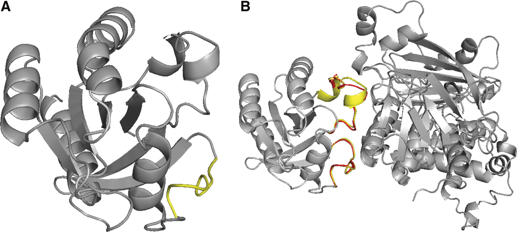
Figure 1 depicts an example of our result. In panel (A), we present a case where many fragment candidates are obtained for the replaceable fragments on the interface of each subunit. The value of Cα RMSD between the unbound and bound states of interface structure is 3.57Å; FlexDoBi gives a candidate of RMSD 2.57Å. In panel (B), multidimensional scaling refines dihedral angles and bond lengths, allowing for more accurate energy calculation. We select the highest ranked structure, which has the iRMSD (the RMSD between the C_α atoms of interface residues) of 2.21Å between the choosing structure and the bound complex.

FIG. 1.

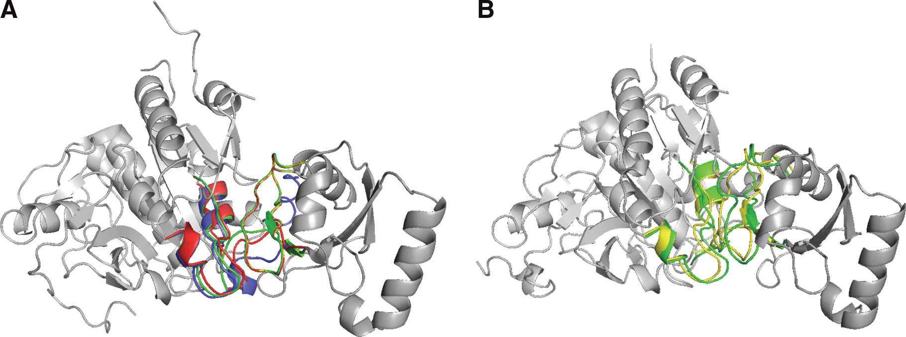
The refinement of the case 2z0e(A:B). (A) The unbound structure of interface is colored green, and several fragment candidates selected by FlexDoBi are colored blue or red. (B) The unbound structure of the interface is colored green, and the refined structure created by FlexDoBi is colored yellow.

3. Results

To evaluate our method, we conduct three groups of experiments. Recall that our method replaces the fragment, which is formed by the consecutive residues, in each interface region with candidate fragments in a database. To test the feasibility of the method, we show that for each native fragment of the bound subunit, there are some similar fragments in the database. The second group of experiments is to examine the performance of our method, that is, the ability of identifying the conformational changes from unbound state to bound state. We use native-bound complexes to fix the pose and compute the conformational changes of interface (see Section 3.2). In Section 3.3, we compare our method (FlexDoBi) with FiberDock (Mashiach et al., 2009), which also assumes that the poses are given. Finally, to test our program for unspecified poses, we compare our method with ZDOCK (Chen et al., 2003).

3.1. Similarity between native interface and selected candidates

Observations of protein complexes show that for many complexes, the major structural changes between the bound and unbound states occur on the interface regions. Our sample data set is extracted from the medium difficulty group (29 complexes) and the regular difficulty group (24 complexes) in protein–protein docking Benchmark 4.0 (Hwang et al., 2010). We calculate the C_α RMSD values on the whole structures and on the interface residues. The average C_α RMSD value between the complex structures and the unbound proteins in native-binding orientation is 1.92Å. However, the average RMSD between the interface residues of these two states is 3.78Å. These details are shown in Figure 2. Clearly, the interfaces are more flexible than the rest of the structures. This justifies our method for transforming an unbound structure into its bound state by substituting only the fragments on the interface.

FIG. 2.

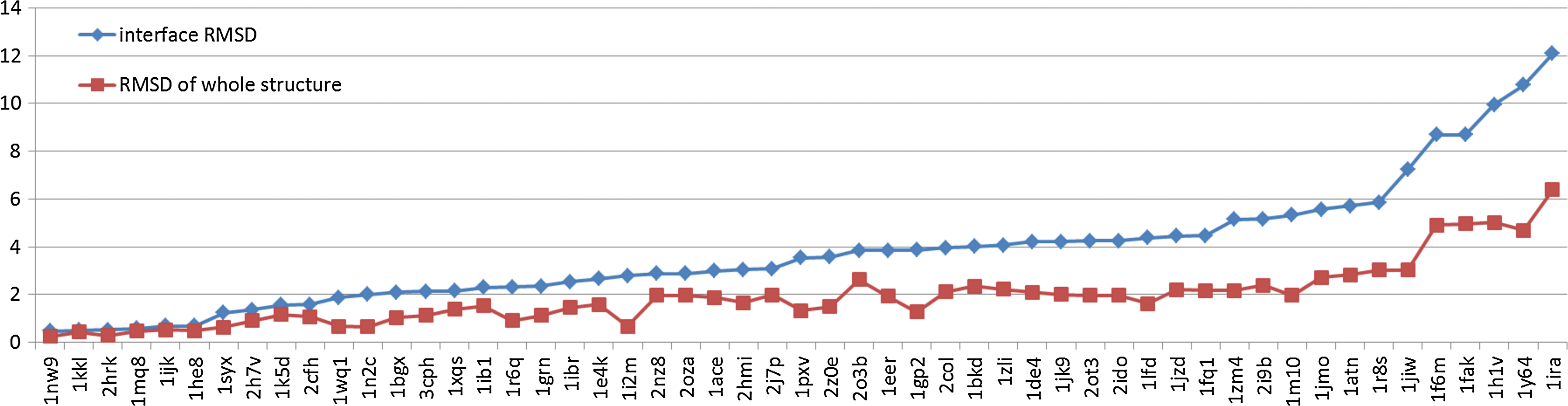
The C_α RMSD between the complex structures and the unbound proteins in native binding orientation: interface RMSD (blue) and RMSD for the whole structure (red).

Suitable replacement fragment candidates are selected from a database. We use a database comprising 13,255 protein chains, selected by using PISCES (Wang and Dunbrack, 2003) with cutoff values being 90 percent identity, resolution 2.0Å, and R-value 0.25. Fragment candidates are selected from this database without the homologous proteins. We find that the homologous candidates appear in the fragment candidates for 42 complexes and filter out those fragments to make a fair assessment. Among 53 complexes, 326 replaceable fragments are extracted from the interfaces of bound states. We search the candidates for the bound state of the replaceable fragment. As shown in Figure 3, for all the fragments, the best candidates are found within 2.25Å.

FIG. 3.

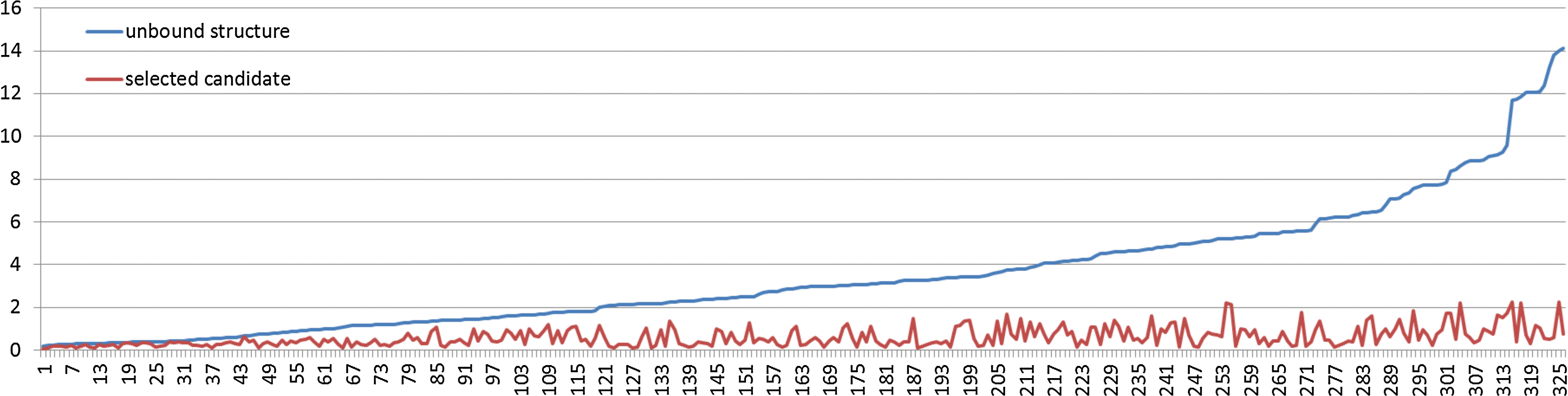
The C_α RMSD between the interface fragments on bound conformations and unbound structures (blue) or best candidates selected by FlexDoBi (red).

3.2. Conformational changes of native poses

In this experiment, we verify that suitable fragment candidates can be identified from the database and reshaped properly for interface fragments. We assume that the native poses are given and two subunits are unbound. Now the task is to transform the unbound subunits onto bound states. To obtain the native pose, the unbound structure is superimposed on the native bound complex by the orientation of lowest C_α RMSD for the whole structure. The value of iRMSD is to denote the RMSD between the C_α atoms of interface in the predicted structure and in the native complex after superimposing the interfaces.

The medium difficulty group in Benchmark 4.0 is used for this study. Details are in Table 1. Among the 29 instances, our program obtains better conformations for 22; that is, FlexDoBi discovers better conformations than simply putting two unbound subunits together for 22 instances. The iRMSD values become worse for three instances and are similar in four instances; by similar, we mean the difference between the iRMSD of the prediction structures and that of the unbound ones is less than 0.05Å. The average C_α iRMSD value between the interface predicted by FlexDoBi and the corresponding portion of the native complex is 2.29Å. Yet, the average iRMSD value between the interface of unbound structures and that of the native complex is 2.51Å.

Table 1.

Refinement of the Unbound Conformations in Their Native Binding Orientations

			FlexDoBi		Unbound ^b
Complex ID	Unbound receptor ^a	Unbound ligand ^a	iRMSD ^c	Energy ^d	iRMSD	Energy
1bgx(HL:T)	1ay1HL	1cmwA	1.97	−287.02	2.10	−233.53
1acb(E:I)	2cgaB	1egl_	2.63	−282.94	2.79	−229.68
1ijk(A:BC)	1auq_	1fvuAB	0.68	−120.15	0.70	−116.70
1jiw(P:I)	1aklA	2rn4A	6.82	−369.11	7.23	−165.38
1kkl(ABC:H)	1jb1AB	2hpr_	0.48	−112.72	0.51	−117.16
1m10(A:B)	1auq_	1m0zB	4.56	−239.47	5.32	−107.04
1nw9(B:A)	1jxqA	2opyA	0.40	−359.64	0.47	−300.06
1gp2(A:BG)	1gia_	1tbgDH	3.76	−236.95	3.86	−160.61
1grn(A:B)	1a4rA	1rgp_	2.44	−366.41	2.35	−228.89
1he8(B:A)	821p_	1e8zA	0.52	−242.02	0.70	−185.29
1i2m(A:B)	1qg4A	1a12A	2.59	−410.51	2.80	−367.41
1ib1(AB:E)	1qjbAB	1kuyA	1.80	−298.37	2.30	−271.32
1k5d(AB:C)	1rrpAB	1yrgB	1.49	−378.72	1.57	−214.85
1lfd(A:B)	5p21A	1lxdA	4.21	−203.56	4.38	−144.88
1mq8(A:B)	1iamA	1mq9A	0.55	−127.40	0.58	−85.25
1n2c(ABCD:EF)	3minABCD	2nipAB	1.68	−234.86	2.01	−169.06
1r6q(A:C)	1r6cX	2w9rA	1.70	−256.47	2.32	−186.50
1syx(A:B)	1qgvA	1l2zA	1.10	−203.26	1.24	−76.83
1wq1(R:G)	6q21D	1wer_	1.61	−379.54	1.87	−328.65
1xqs(A:C)	1xqrA	1s3xA	2.13	−363.10	2.15	−278.70
1zm4(A:B)	1n0vC	1xk9A	5.03	−278.57	5.15	−180.03
2cfh(A:C)	1sz7A	2bjnA	1.49	−298.42	1.59	−248.20
2h7v(A:C)	1mh1_	2h7oA	1.12	−263.02	1.36	−208.97
2hrk(A:B)	2hraA	2hqtA	0.76	−241.75	0.52	−237.32
2j7p(A:D)	1ng1A	2iylD	3.15	−491.82	3.09	−393.70
2nz8(A:B)	1mh1_	1ntyA	2.67	−383.72	2.88	−312.00
2oza(B:A)	3hecA	3fykX	2.69	−549.15	2.89	−221.08
2z0e(A:B)	2d1iA	1v49A	2.21	−343.12	3.57	−229.21
3cph(A:G)	3cpiG	1g16A	2.07	−303.29	2.13	−309.73

Unbound structure of receptor or ligand in the complex.

Unbound structure is superimposed on the bound conformation by the orientation of lowest C_α RMSD for the whole structure.

C_α RMSD between the interface of the predicted structure and the native complex.

Energy value of the predicted complex.

The best instances, predicted by FlexDoBi, are 1m10(A:B), 1r6q(A:C), and 2z0e(A:B), where the values of C_α iRMSD are reduced by 0.7Å, 0.6Å, and 1.3Å, respectively. Figure 4 displays the conformation discovered by FlexDoBi for 1r6q(A:C). FlexDoBi predicts the interface conformation with 1.70Å iRMSD; however, the value of iRMSD for the unbound structures on the native orientation is 2.32Å. The energy of the conformation predicted by FlexDoBi, −256.47, is lower than the initial energy of the unbound structure, −186.50. We should notice that lower energy does not always imply better conformation in terms of iRMSD.

FIG. 4.

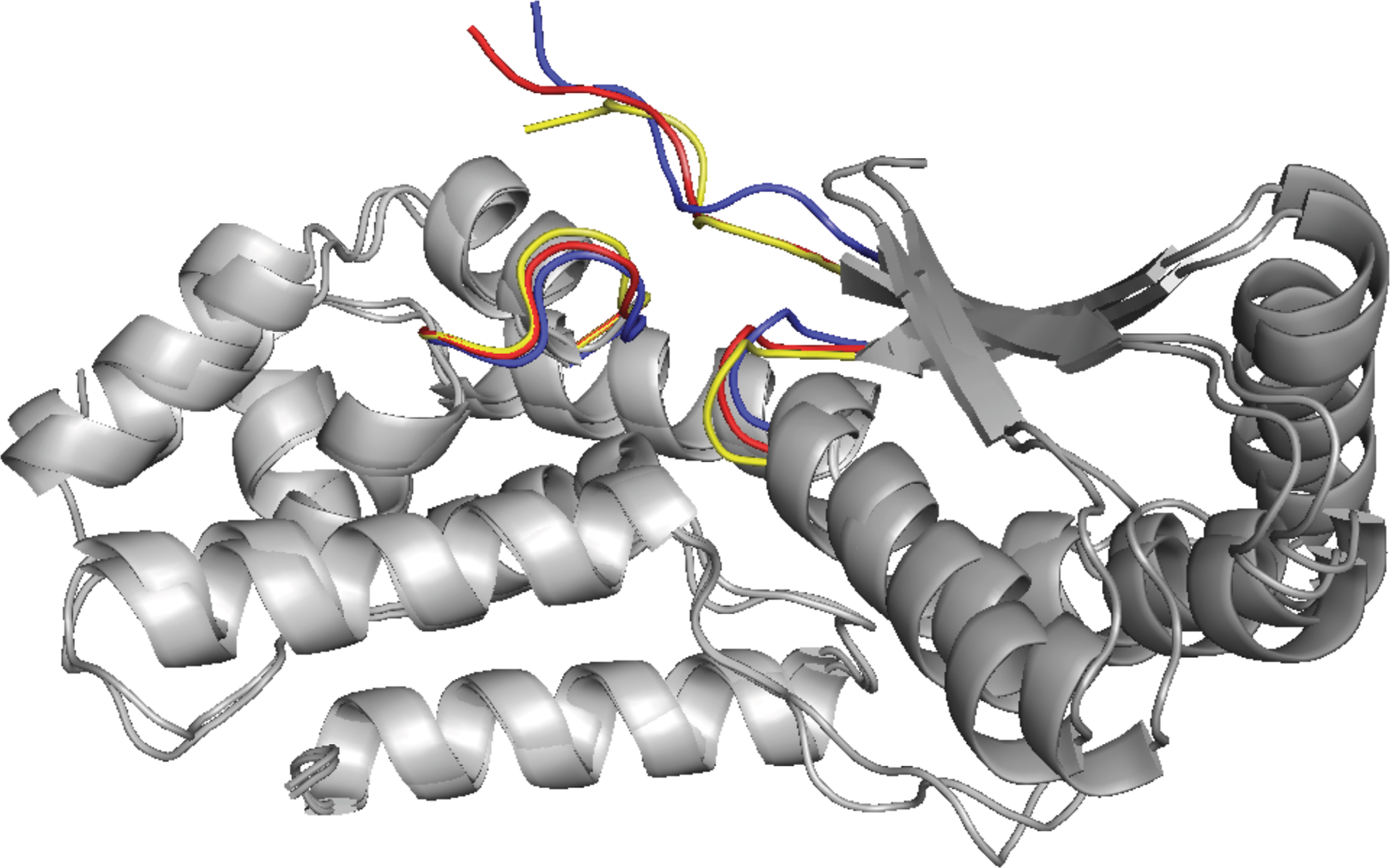
The refinement of the case 1r6q(A:C): The unbound structure of interface is colored yellow and the bound structure is blue. The refined structure, created by FlexDoBi, is in red.

3.3. Comparison with FiberDock

In this subsection, we compare the results of FlexDoBi with FiberDock (Mashiach et al., 2009). FiberDock is a novel NMA-based backbone flexibility treatment, which refines the structure of complex from a given docking configuration. We evaluate the performance of two methods by using the unbound native pose. The data set is extracted from FiberDock's paper. We obtain much better results than that of FiberDock. The comparison result is detailed in Table 2. Among 20 instances, FlexDoBi produces better results for 14 instances. By better, we mean that the iRMSD value is at least 0.05Å smaller than the iRMSD of the FiberDock method. Only for four instances, FiberDock produces better results. The average values of C_α iRMSD between the predicted structures and the native complexes are 1.55Å (FlexDoBi) and 1.94Å (FiberDock), respectively.

Table 2.

Docking Results of FlexDoBi and FiberDock with Known Poses

			FlexDoBi		FiberDock
Complex ID	Unbound receptor ^a	Unbound ligand ^a	iRMSD ^c	rec-iRMSD ^d	iRMSD	rec-iRMSD	Unbound ^b
1a0o(A:B)	1chn_	1fwpA	3.19	3.68	2.44	2.12	3.27
1acb(E:I)	2cgaB	1egl_	2.63	2.85	2.58	2.54	2.79
1ay7(A:B)	1rghB	1a19B	0.47	0.40	1.30	0.59	0.43
1bth(H:P)	2hnt_	6ptiA	1.34	1.67	1.16	1.31	1.49
1cgi(E:I)	2cgaB	1hpt_	2.09	2.28	2.08	2.26	2.53
1dfj(E:I)	9rsa_	2bnh_	0.56	0.53	1.12	1.11	0.56
1e6e(A:B)	1e1nA	1cjeD	0.64	0.84	1.21	0.62	0.73
1fin(A:B)	1hcl_	1vin_	5.47	7.47	6.06	6.16	5.17
1ggi(L:H)	1ggcL	1cgiH	0.66	1.08	1.95	1.26	0.71
1got(A:B)	1tag_	1tbgA	0.92	1.35	4.68	3.78	3.62
1ibr(A:B)	1qg4A	1f59A	2.37	1.27	2.63	2.56	2.53
1oaz(H:L)	1oaqH	1oazL	0.75	0.50	1.00	1.07	0.70
1pxv(A:C)	1x9yA	1nycA	2.90	3.79	3.42	3.31	3.85
1t6g(C:A)	1ukr_	1t6e_	0.48	0.37	0.88	0.66	1.10
1tgs(Z:I)	2ptn_	1hpt_	0.64	0.56	1.57	1.54	1.38
1wq1(R:G)	6q21D	1wer_	1.61	1.79	1.50	0.93	1.87
1zhi(A:B)	1m4zA	1z1aA	0.75	1.10	1.24	0.74	0.94
2buo(A:T)	1a43_	2buoT	1.24	0.54	4.05	4.30	1.96
2kai(A:I)	2pka_	6pti_	0.38	0.34	0.74	0.72	0.31
3hhr(A:B)	1hgu_	3hhrB	2.93	3.56	1.98	2.56	2.94

Unbound structure of receptor or ligand in the complex.

Unbound structure is superimposed on the bound conformation by the orientation of lowest C_α RMSD for the whole structure.

C_α RMSD between the interface in the predicted structure and the native complex.

C_α RMSD between the interface in the predicted structure of receptor and in its bound conformation.

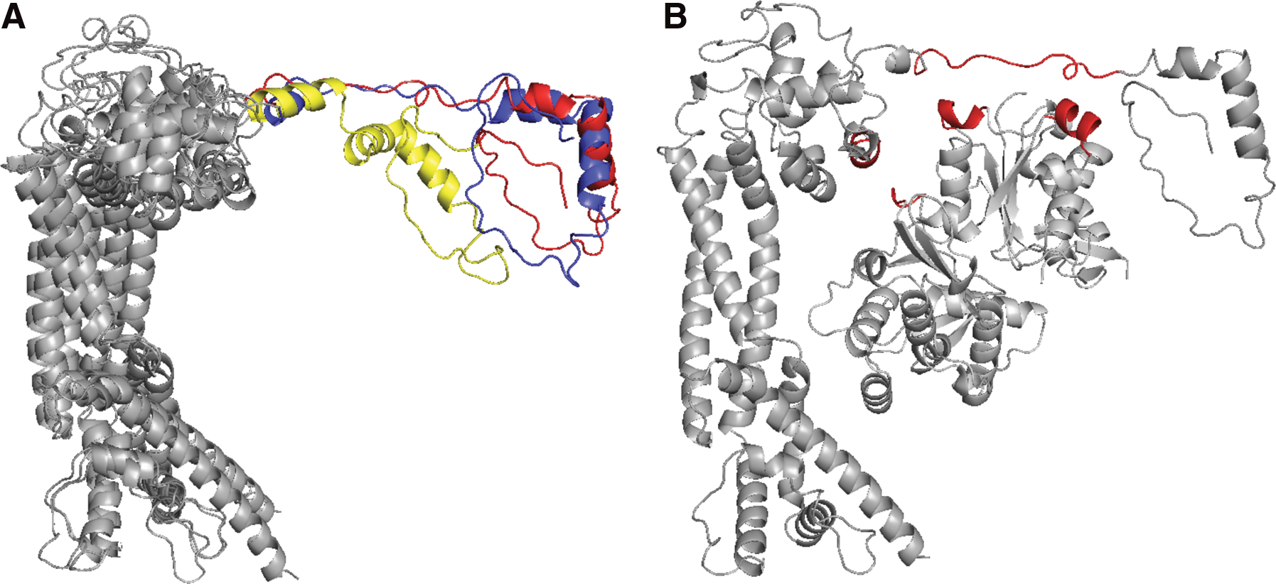
Rec-iRMSD is to denote the iRMSD value of the receptor, which is the subunit of more residues. The average values of Rec-iRMSD between the predictions and the bound conformations are 1.71Å (FlexDoBi) and 2.01Å (FiberDock), respectively. In case of 1got(A:B), FlexDoBi predicts new interface conformation in complex with 0.92Å C_α iRMSD, however, the value of iRMSD for the unbound structures on the native orientation is 3.62Å. Figure 5 displays the docking configuration discovered by FlexDoBi for 1got(A:B). The comparisons indicate that FlexDoBi produces better interface conformations while changing the unbound states into bound states.

FIG. 5.

The refinement of the case 1got(A:B): The unbound structure of interface is colored yellow and the bound structure is blue. The refined structure, created by FlexDoBi, is in red.

3.4. Evaluation on Benchmark v4.0

In this study, we assume that the native pose is unknown. We perform a search that finds both the poses and identifies the structural changes. For each complex, we adopt a similar procedure as in P-Binder to predict the poses. The top 100 poses according to our new energy function are chosen and are fed into our method for modeling conformational changes. The top ten results from the method according to energy value are reported. These are finally compared with the docking results from ZDOCK (Chen et al., 2003), and the flexible docking solutions from FiberDock, which refines the poses predicted by ZDOCK. In order to test the refining ability of our method, we use FlexDoBi to model the conformational changes of the poses predicted by ZDOCK. The docking results are shown in Table 3. In general, the iRMSD values decrease as the magnitude of conformational change increases.

Table 3.

Docking Results of FlexDoBi, ZDOCK, and FiberDock on Benchmark v4.0

Type	No. of cases	FlexDoBi ^a	ZDOCK ^a	FlexDoBi-r ^b	FiberDock ^b
Rigid body	123	3.96	4.15	—	—
Medium difficulty	29	4.61	4.96	4.79	4.88
Difficult	24	7.78	8.59	7.85	7.84
Overall	176	4.63	4.89	4.75	4.77

C_α iRMSD between the predicted configuration by each method and the native complex.

C_α iRMSD between the changed conformation predicted by each method and the native complex, refining the best pose of ZDOCK.

We compare our method with ZDOCK on the rigid-body group in Benchmark v4.0. The values of C_α iRMSD between the unbound structures in the native poses and the native complexes range from 0.24Å to 2.02Å. The results are presented in Table 4. For 123 complexes in the rigid-body group, the average C_α iRMSD values between the predictions and the native complexes are 3.96Å (FlexDoBi) and 4.15Å (ZDOCK), respectively. FlexDoBi produces better results for 82 instances than ZDOCK.

Table 4.

Docking Results of FlexDoBi and ZDOCK on the Rigid-Body Group

Complex	FlexDoBi ^a	ZDOCK ^a	Complex	FlexDoBi	ZDOCK	Complex	FlexDoBi	ZDOCK
1ahw	2.51	8.91	1oc0	1.48	3.20	1he1	1.21	2.30
1bvk	1.58	3.73	1oph	2.33	4.16	1i4d	1.98	1.96
1dqj	3.62	5.60	1oyv^c	2.23	1.30	1j2j	1.76	2.18
1e6j	1.45	1.71	1oyv^c	2.89	1.68	1jwh	17.52	1.90
1jps	16.36	7.88	1ppe	1.54	0.77	1k74	0.75	2.30
1mlc	8.48	1.54	1r0r	2.77	6.29	1kac	2.10	6.82
1vfb	2.61	4.10	1tmq	1.15	1.78	1klu	2.97	6.77
1wej	1.32	1.16	1udi	1.09	1.46	1ktz	3.51	7.06
2fd6	0.82	2.04	1yvb	2.60	1.07	1kxp	1.60	1.92
2i25	1.49	1.74	2abz	3.18	5.94	1ml0	0.88	1.23
2vis	17.31	7.71	2b42	1.05	1.07	1ofu	7.29	1.89
1bj1	1.20	1.07	2j0t	1.46	3.26	1pvh	2.37	6.59
1fsk	0.67	1.11	2mta	2.26	2.48	1qa9	2.23	12.15
1i9r	1.26	2.28	2o8v	1.65	3.66	1rlb	14.50	1.68
1iqd	0.78	0.79	2oul	0.81	1.24	1rv6	10.55	1.60
1k4c	2.50	4.90	2pcc	14.13	3.45	1s1q	16.10	7.10
1kxq	0.90	1.16	2sic	1.53	0.64	1sbb	3.54	8.77
1nca	1.38	1.04	2sni	0.61	1.91	1t6b	3.90	10.27
1nsn	3.37	5.41	2uuy	2.86	3.74	1us7	1.03	3.58
1qfw^b	2.76	14.24	3sgq	1.38	2.60	1wdw	2.18	1.54
1qfw^b	10.30	10.12	4cpa	2.03	2.39	1xd3	1.68	1.90
2jel	1.19	1.53	7cei	1.64	0.95	1xu1	18.83	2.92
1avx	0.65	1.48	1a2k	18.60	3.81	1z0k	2.62	1.94
1ay7	1.75	4.17	1ak4	16.90	5.89	1z5y	1.99	1.78
1bvn	1.16	1.39	1akj	5.89	14.89	1zhh	15.70	14.96
1cgi	3.19	2.27	1azs	1.06	1.18	1zhi	1.83	1.72
1clv	1.11	1.38	1b6c	1.97	2.30	2a5t	3.19	7.68
1d6r	2.13	5.42	1buh	15.92	1.53	2a9k	1.02	8.72
1dfj	1.11	1.37	1e96	2.47	3.20	2ajf	4.29	3.26
1e6e	3.12	1.42	1efn	3.95	5.94	2ayo	4.89	1.89
1eaw	1.60	1.49	1f51	2.98	1.13	2b4j	4.13	5.86
1ewy	1.18	2.54	1fc2	3.10	11.44	2btf	1.25	6.62
1ezu	2.75	3.28	1fcc	2.56	10.97	2fju	2.47	5.81
1f34	5.41	10.59	1ffw	1.81	3.50	2g77	2.38	2.44
1fle	1.78	2.67	1fqj	4.03	9.75	2hle	2.02	2.58
1gl1	2.13	1.46	1gcq	12.12	8.03	2hqs	1.18	8.59
1gxd	6.97	10.01	1ghq	6.46	12.40	2oob	4.98	7.94
1hia	1.26	4.25	1gla	5.63	4.11	2oor	3.68	6.90
1jtg	2.30	1.33	1gpw	2.40	1.41	2vdb	3.64	5.68
1mah	0.69	1.02	1h9d	1.62	4.05	3bp8	4.50	8.84
1n8o	1.12	1.27	1hcf	17.80	2.42	3d5s	1.70	1.73

C_α iRMSD between the predicted configuration of each method and the native complex.

The first complex is 1qfw(HL:AB), and the second complex is 1qfw(IM:AB).

The first complex is 1oyv(B:I), and the second complex is 1oyv(A:I).

We calculate the medium difficulty group and the regular difficulty group in Benchmark v4.0. The values of C_α iRMSD between the unbound structures in the native poses and the native complexes range from 1.48Å to 16.76Å. Several proteins in the regular difficulty group undergo significant conformational changes upon binding. The results are presented in Tables 5 and 6.

Table 5.

Docking Results of FlexDoBi, ZDOCK, and FiberDock on Medium Difficulty Group

Complex	FlexDoBi ^a	ZDOCK ^a	FlexDoBi-r ^b	FiberDock ^b	Complex	FlexDoBi	ZDOCK	FlexDoBi-r	FiberDock
1bgx	9.83	11.90	10.86	9.82	1n2c	6.75	3.21	2.96	3.51
1ace	5.46	2.61	2.12	3.16	1r6q	3.93	5.20	4.63	4.38
1ijk	4.17	1.86	1.57	1.22	1syx	6.97	4.81	4.06	2.04
1jiw	7.49	8.22	6.85	5.93	1wq1	2.06	1.82	2.45	2.64
1kkl	3.18	17.92	16.98	15.53	1xqs	2.76	2.67	2.12	2.25
1m10	5.87	9.42	7.34	6.26	1zm4	5.96	2.44	3.14	3.67
1nw9	3.49	3.19	3.65	5.06	2cfh	4.18	1.53	1.9	1.69
1gp2	4.18	3.39	2.19	1.70	2h7v	4.02	2.64	2.01	2.36
1grn	3.49	1.81	1.73	2.31	2hrk	2.35	2.06	1.78	1.56
1he8	4.76	2.38	2.24	2.34	2j7p	4.86	6.89	7.52	8.65
1i2m	4.24	2.21	2.37	2.96	2nz8	5.17	2.87	2.33	1.81
1ib1	7.19	5.89	6.52	7.60	2oza	4.89	8.49	8.27	8.69
1k5d	2.16	2.51	2.97	4.94	2z0e	3.64	4.24	4.53	6.87
1lfd	6.21	4.94	4.32	4.04	3cph	3.27	3.91	4.29	4.16
1mq8	2.99	6.72	6.51	8.19

C_α iRMSD between the predicted configuration of each method and the native complex.

C_α iRMSD between the changed conformation predicted by each method and the native complex, refining the best pose of ZDOCK.

Table 6.

Docking Results of FlexDoBi, ZDOCK, and FiberDock on Difficulty Group

Complex	FlexDoBi ^a	ZDOCK ^a	FlexDoBi-r ^b	FiberDock ^b	Complex	FlexDoBi	ZDOCK	FlexDoBi-r	FiberDock
1e4k	9.42	15.20	13.58	8.71	1h1v	16.13	16.72	13.97	14.53
2hmi	6.14	16.99	12.62	13.46	1ibr	8.23	9.83	9.27	8.86
1f6m	5.76	12.24	10.21	12.33	1ira	20.13	16.42	13.1	12.48
1fq1	5.54	8.05	7.28	7.61	1jk9	5.69	2.16	1.62	2.77
1pxv	5.17	3.81	4.06	3.82	1jmo	11.01	15.99	11.46	10.52
1zli	6.97	12.25	10.95	9.86	1jzd	7.92	16.70	12.05	11.59
2o3b	9.15	14.16	11.27	9.37	1r8s	6.23	6.48	4.87	6.86
1atn	4.70	4.74	3.92	4.27	1y64	6.42	14.37	12.51	15.31
1bkd	7.04	7.33	6.47	6.38	2c0l	5.14	4.36	3.34	5.05
1de4	6.76	1.77	1.26	1.49	2i9b	4.18	5.58	4.13	4.75
1eer	7.49	7.90	7.2	5.40	2ido	5.48	5.09	4.25	3.42
1fak	6.73	7.73	6.85	7.44	2ot3	9.11	4.40	3.17	3.25

C_α iRMSD between the predicted configuration of each method and the native complex.

C_α iRMSD between the changed conformation predicted by each method and the native complex, refining the best pose of ZDOCK.

For 29 complexes in the medium difficulty group, the average C_α iRMSD values between the poses predicted by FlexDoBi and the native complexes is 4.61Å. ZDOCK predicts the best poses with 4.96Å iRMSD; FlexDoBi and FiberDock refine the best poses with 4.79Åand 4.88Å iRMSD, respectively. FlexDoBi computes better changed conformations for 16 instances than FiberDock, for refining the best poses predicted by ZDOCK. For 24 complexes in the regular difficulty group, the average C_α iRMSD values between the poses predicted by FlexDoBi and the native complexes is 7.78Å. ZDOCK predicts the best poses with 8.59Å iRMSD, FlexDoBi and FiberDock refine the best poses with 7.85Åand 7.84Å iRMSD, respectively. FlexDoBi computes better changed conformations than FiberDock for 12 instances.

In several unbound subunits, the coordinates of some backbone atoms are missing. We add the coordinates of the missing residues using MODELLER (Eswar et al., 2006). In two groups, the missing residues appear in the unbound structures of four complexes: residues 36–43 in 1fq1B, residues 206–215 in 1grnB, residues 72–94 in 1jmoA, and residues 46–58 in 3cphA. After the gaps are filled in, the accuracy of the predictions is improved. The docking configuration discovered by FlexDoBi for 3cph(A:G), after the gap is filled, is displayed in Figure 6. The complex predicted by FlexDoBi has an iRMSD of 3.27Å C_α, which is better than the iRMSD of 3.91Å from ZDOCK.

FIG. 6.

The refinement of case 3cph(A:G). (A) The missing residues in the unbound structure of 3cphA are filled by MODELLER (yellow). (B) The unbound structure of the interface is colored yellow. The refined structure, created by FlexDoBi, is in red.

3.5. Assessment of the energy items

To assess the effectiveness of the energy items, we analyze the performance with Benchmark v4.0. For evaluating the effectiveness of energy items, we reoptimize the coefficients in each case with only four out of five items and reevaluate the predicted structures by leaving one energy item out. The iRMSD without side-chain energy is 4.72Å, without dDFIRE energy function is 4.77Å, without atomic contact energy is 4.66Å, without secondary structure energy is 4.78Å, and without the Gromacs force field is 4.71Å. The C_α iRMSD of all the above five experiments are worse than with all energy items, 4.63Å. It is clear that dDFIRE energy function and secondary structure energy have more impact.

4. Method Details

4.1. Selecting candidates from the database

We exam the known protein structures and identify suitable candidates to replace each fragment on the interface. We use a database of 13,255 protein chains, selected by using PISCES (Wang and Dunbrack, 2003), with cutoff values of 90 percent identity, 2.0Å resolution, and 0.25 R-value (Sept. 2012). Fragment candidates are selected from this database without the homologous proteins. We look for the fragment candidates whose stems are within 3Å to the stems of replaceable fragments. Once fragment candidates are obtained, we take the top 100 fragments according to the sequence similarity as the matching candidates. The sequence similarity is computed according to BLOSUM62 matrix. As the replaceable fragment and the candidates have the same number of residues, the sequence similarity is the sum of the respective residue pair values in the matrix.

4.2. Fitting candidates on replaceable fragment

We cannot replace the fragments by the candidates directly, as it will result in unrealistic atomic distances and clashes. We scale the candidates to resolve those issues.

We formulate this structure problem as an instance of weighted multidimensional scaling (WMDS). For a given d dimension and n points of data, we have a distance matrix D and a weighted matrix W, both symmetric n × n matrixes, and wish to find \documentclass{aastex}\usepackage{amsbsy}\usepackage{amsfonts}\usepackage{amssymb}\usepackage{bm}\usepackage{mathrsfs}\usepackage{pifont}\usepackage{stmaryrd}\usepackage{textcomp}\usepackage{portland, xspace}\usepackage{amsmath, amsxtra}\pagestyle{empty}\DeclareMathSizes{10}{9}{7}{6}\begin{document} $$X = \{ x_{1} , x_{2} , \ldots , x_{n} \} $$ \end{document} where x_i is a coordinate in d dimension, such that we minimize the stress, defined as δ(X) = ∑_0<i<j≤nW_i,j(||x_i−x_j||−D_i,j)². WMDS can be used to turn high-dimensional data into 2- or 3-dimensional data suitable for graphing. It has also been used in LoopWeaver (Holtby et al., 2012) for modeling loop structures, and MUFOLD (Zhang et al., 2010) for assembling protein fragments.

For our problem instances, d = 3 and n is the total number of backbone atoms in all replaceable fragments and the stems on the interface of two subunits A and B. We define the distance matrix D as \documentclass{aastex}\usepackage{amsbsy}\usepackage{amsfonts}\usepackage{amssymb}\usepackage{bm}\usepackage{mathrsfs}\usepackage{pifont}\usepackage{stmaryrd}\usepackage{textcomp}\usepackage{portland, xspace}\usepackage{amsmath, amsxtra}\pagestyle{empty}\DeclareMathSizes{10}{9}{7}{6}\begin{document} \begin{align*}d_{i , j} = \begin{cases} \mid \mid t_{i} - t_{j} \mid \mid \qquad i , j \ \in \ stem \\ \mid \mid c_{i} - c_{j} \mid \mid \qquad otherwise\end{cases}\end{align*} \end{document}

where \documentclass{aastex}\usepackage{amsbsy}\usepackage{amsfonts}\usepackage{amssymb}\usepackage{bm}\usepackage{mathrsfs}\usepackage{pifont}\usepackage{stmaryrd}\usepackage{textcomp}\usepackage{portland, xspace}\usepackage{amsmath, amsxtra}\pagestyle{empty}\DeclareMathSizes{10}{9}{7}{6}\begin{document} $$T = \{ t_{1} , t_{2} , \ldots , t_{n} \} $$ \end{document} is the set of atomic coordinates in the protein, and \documentclass{aastex}\usepackage{amsbsy}\usepackage{amsfonts}\usepackage{amssymb}\usepackage{bm}\usepackage{mathrsfs}\usepackage{pifont}\usepackage{stmaryrd}\usepackage{textcomp}\usepackage{portland, xspace}\usepackage{amsmath, amsxtra}\pagestyle{empty}\DeclareMathSizes{10}{9}{7}{6}\begin{document} $$C = \{ c_{1} , c_{2} , \ldots , c_{n} \} $$ \end{document} is the set of atomic coordinates in the candidate structure. In the candidate structure, we choose one of the matching candidates instead of each replaceable fragment.

The distances are unequally important, so we adopt a weighted version. First, the stem atoms are fixed, so the pairwise weights between each pair of stem atoms must be large. Moreover, neighboring atoms should be given larger weights, because they represent bond lengths. If two atoms are within a small distance, then they should remain close to this distance regardless of other changes, especially if they are adjacent backbone atoms. On the contrary, distant atoms are free to move around. The weighted matrix is defined as \documentclass{aastex}\usepackage{amsbsy}\usepackage{amsfonts}\usepackage{amssymb}\usepackage{bm}\usepackage{mathrsfs}\usepackage{pifont}\usepackage{stmaryrd}\usepackage{textcomp}\usepackage{portland, xspace}\usepackage{amsmath, amsxtra}\pagestyle{empty}\DeclareMathSizes{10}{9}{7}{6}\begin{document} \begin{align*}w_{i , j} = \begin{cases}1000 \qquad \qquad \qquad \qquad \qquad i , j \in stem \\ T ( i \ { \rm mod} \ 4 , j - i ) \qquad \qquad i , j \in f_{s} , j - i \leq 4 \\ ( \min \{ d_{i , j} , r - \Phi d_{i , j} \} ) ^{ - 2} \quad i , j \in f_{s} , j - i > 4 \\ d_{i , j}^{ - 2} \qquad \qquad \qquad \qquad \qquad \qquad i , j \in f_{d} \\ 0 \qquad \qquad \qquad \qquad \qquad \ \qquad otherwise\end{cases}\end{align*} \end{document}

where 0 ≤ i < j ≤ n, T is a 4 × 4 lookup table as defined in LoopWeaver (Holtby et al., 2012), r is the largest pairwise distance between any two atoms in the corresponding matching candidate, and Φ is the golden ratio conjugate. In addition, \documentclass{aastex}\usepackage{amsbsy}\usepackage{amsfonts}\usepackage{amssymb}\usepackage{bm}\usepackage{mathrsfs}\usepackage{pifont}\usepackage{stmaryrd}\usepackage{textcomp}\usepackage{portland, xspace}\usepackage{amsmath, amsxtra}\pagestyle{empty}\DeclareMathSizes{10}{9}{7}{6}\begin{document} $$i , j \in f_s$$ \end{document} denotes that two atoms i and j belong to the same fragment and \documentclass{aastex}\usepackage{amsbsy}\usepackage{amsfonts}\usepackage{amssymb}\usepackage{bm}\usepackage{mathrsfs}\usepackage{pifont}\usepackage{stmaryrd}\usepackage{textcomp}\usepackage{portland, xspace}\usepackage{amsmath, amsxtra}\pagestyle{empty}\DeclareMathSizes{10}{9}{7}{6}\begin{document} $$i , j \in f_d$$ \end{document} denotes two atoms i and j belong to two different fragments. If two atoms belong to two different fragments, they must satisfy one of the following requirements: (1) two fragments, one from each subunit, interact with each other; and (2) two fragments, both from the same subunit, interact with the same fragment of another subunit. The weight between atoms of the same fragment is the same as in LoopWeaver. For two different fragments, the interacting residues and the surrounding regions can move freely while having a minor effect on the contribution to the stress function. We set the weight to \documentclass{aastex}\usepackage{amsbsy}\usepackage{amsfonts}\usepackage{amssymb}\usepackage{bm}\usepackage{mathrsfs}\usepackage{pifont}\usepackage{stmaryrd}\usepackage{textcomp}\usepackage{portland, xspace}\usepackage{amsmath, amsxtra}\pagestyle{empty}\DeclareMathSizes{10}{9}{7}{6}\begin{document} $$d_{i , j}^{ - 2}$$ \end{document} when atoms i and j belong to different fragments, because pairs of closer atoms are more significant than pairs of relatively farther atoms when refining the conformation structures.

We use the SMACOF algorithm (de Leeuw, 1977) for solving the WMDS problem. This algorithm works by minimizing the stress function and yielding a fast, deterministic heuristic. By performing the iterative generation, the quality of interface refinement often gets better, and the unrealistic atomic distances are eliminated in the candidate structure.

4.2.1. Searching best conformations

Given a pair of subunits, we extract a candidate set for each replaceable fragment. For each replaceable fragment, at most 100 candidates are chosen. Then we replace the fragments by the candidates from the respective candidate set randomly. If a better conformation according to the energy function is found, we keep it. Otherwise, we try to replace a fragment by other candidates. This process is repeated until convergence. We restart the above procedure to generate multiple structure candidates. We use SCWRL4 to build the side-chain conformation of these structure candidates and evaluate them by the dDFIRE energy function.

4.3. Energy items

Our method generates a large number of structure candidates. Here we develop a new energy function to select the best structures. Our energy function contains the following energy items:

(1) The side-chain atoms of interface residues are packed by SCWRL4 (Krivov et al., 2009), and the corresponding energy item is extracted.

(2) The dDFIRE energy is an all-atom statistical function (Yang and Zhou, 2008) based on the atomic distance and three orientation angles involved in dipole–dipole interactions.

(3) The item of atomic contact energy is produced by an atomic energy measure (Zhang et al., 1997; Zhang, 1998). The free energy for a pair of interacting atoms has been calculated on atom-pairing frequencies in known complexes.

(4) We use DSSP (Kabsch and Sander, 1983) to determine the type of secondary structure for each residue and construct the item of secondary structure energy by using the statistical method in Guo et al. (2012). Here, we incorporate three types of secondary structures, 20 types of amino acids, and one solvent contacting the residues in protein surfaces. The secondary structure energy item takes 60 × 60 possible residue pairs, obtained from the statistical analysis of residue-pairing frequencies in a complex database. We select 6,323 complexes from PDB database, and these complexes are made up of two or more protein subunits. Their structures are determined by X-rays with cutoff values of resolution 2.2Å and sequence identity 30% (Sept. 2012). We calculate the free energy for all pairs of interacting residues in candidate structures.

(5) The Gromacs force field is built up from two distinct subunits to describe the interaction between their atoms (Lindahl et al., 2001). Gromacs calculates electrostatic interactions in the standard coulomb potential as

\documentclass{aastex}\usepackage{amsbsy}\usepackage{amsfonts}\usepackage{amssymb}\usepackage{bm}\usepackage{mathrsfs}\usepackage{pifont}\usepackage{stmaryrd}\usepackage{textcomp}\usepackage{portland, xspace}\usepackage{amsmath, amsxtra}\pagestyle{empty}\DeclareMathSizes{10}{9}{7}{6}\begin{document} \begin{align*}F ( r_ { ij } ) = f \frac { q_ { i } q_ { j } } { \varepsilon_ { r } r_ { ij } ^ { 2 } } \hat { r } _ { ij }\end{align*} \end{document}

where \documentclass{aastex}\usepackage{amsbsy}\usepackage{amsfonts}\usepackage{amssymb}\usepackage{bm}\usepackage{mathrsfs}\usepackage{pifont}\usepackage{stmaryrd}\usepackage{textcomp}\usepackage{portland, xspace}\usepackage{amsmath, amsxtra}\pagestyle{empty}\DeclareMathSizes{10}{9}{7}{6}\begin{document} $$\hat{r}_{ij}$$ \end{document} is the unit vector, parallel with the line from charge q_i to charge q_j, and \documentclass{aastex}\usepackage{amsbsy}\usepackage{amsfonts}\usepackage{amssymb}\usepackage{bm}\usepackage{mathrsfs}\usepackage{pifont}\usepackage{stmaryrd}\usepackage{textcomp}\usepackage{portland, xspace}\usepackage{amsmath, amsxtra}\pagestyle{empty}\DeclareMathSizes{10}{9}{7}{6}\begin{document} $$r_ { ij } = r_ { j } - r_ { i } ; \,f = \frac { 1 } { 4 \pi \varepsilon_ { 0 } } = 138.9$$ \end{document} , and ɛ_r is the relative dielectric constant in Gromacs.

We use a linear combination of these energy items to rank the poses and to direct the search for finding the plausible conformations. The coefficient of each item is optimized by using a training set. Details are described as following. For a pair of subunits, we generate 1,000 candidate poses. The top 200 poses according to the iRMSD values are selected. The energy values of these 200 poses are computed. Then we choose the top 10 poses according to the combined energy value. The objective here is to minimize the sum of the iRMSD values of the top 10 candidates for the training set. The grid search method is used (Al-Khayyal, 1990). We identify the best possible combination of coefficients from 0.1 to 10. For the values of range 0.1 to 1, we use a step size of 0.1. For the values ranging from 1 to 10, we use a step size of 1.0. After we obtain the best combination of coefficients, we refine them further by allowing higher resolution. We change the coefficient by ±0.5 with a step size of 0.1. The optimal combination of coefficients is used for prediction on the testing set.

Finally, we use a trained SVM regression model to rank the docking solutions and report the best ones with the lowest predicted values. For the training set, we use iRMSD as the response values for all configurations of each protein pair, and the above energy items can be regarded as five features for each one. The configurations with the lowest predicted response values can be reported as results on the testing set. To obtain the parameters, we use 36 unbound–unbound complexes from Dockground (Liu et al., 2008) as the training set, which are not included in the testing set.

5. Conclusion and Discussion

In this article, we present a new method for flexible refinement of docking solutions. We formulate the backbone flexibility problem on the interface as an instance of the weighted multidimensional scaling problem, which is able to model the local conformational changes. The results show that FlexDoBi models the backbone motions on the protein–protein interface. The backbone refinement procedure improves the accuracy of near-native docking solution candidates.

Our method can eliminate a larger number of inaccurate candidate structures due to the geometrical constraints imposed by the distance between two residues respectively at both ends of each interface fragment. However, we only deal with the cases in which the regions far from the interface should be almost unchanged in complex.

We notice that large conformation changes can occur and result in a whole structure of interacting proteins. On the regular difficulty group, the large changes appear in the unbound structures of three complexes: 1y64(A:B), 1f6m(A:C), and 1ira(Y:X). In the case of 1y64B, the conformational change occurs in the loop region (residues 1396–1416). First, we replace this loop region with all loop candidates in the protein database, regardless of the stem RMSD value. Then, we also refine the interface conformation of complex by using our flexible docking method in this article. The best discovered configuration is displayed in Figure 7. We predict a new configuration of complexes with 6.42Å C_α iRMSD, whereas the value of iRMSD for the predicted complex without the replaced loop is 11.77Å. Those issues will be our further investigations in the near future.

FIG. 7.

The refinement of case 1y64(A:B): (A) The unbound structure is colored yellow, and the bound structure is blue. The replaced loop is in red. (B) The refined interface structure is in red.

Footnotes

Acknowledgments

This work is supported by the grants from the Research Grants Council of the Hong Kong Special Administrative Region, China [Project No. CityU 124512], and the startup fund [Project No. 7200276] and grant [Project No. 9610025] from the City University of Hong Kong.

Author Disclosure Statement

No competing financial interests exist.

References

Alcaro

, Gasparrini

, Incani

et al. 2007. “Quasi flexible” automatic docking processing for studying stereoselective recognition mechanisms, part 2: Prediction of deltadeltag of complexation and 1h-nmr noe correlation. Journal of Computational Chemistry, 28:1119–1128.

Al-Khayyal

1990. Jointly constrained bilinear programs and related problems: an overview. Computers and Mathematics with Applications, 19:53–62.

Bradford

J.R.

, Westhead

D.R.

2005. Improved prediction of protein-protein binding sites using a support vector machines approach. Bioinformatics, 21:1487–1494.

Brown

J.B.

, Bahadur

, Tomita

, Akutsu

2006. Multiple methods for protein side chain packing using maximum weight cliques. Genome Informatics, 3:191–200.

Chen

, Li

, Weng

2003. Zdock: an initial-stage protein-docking algorithm. Proteins, 52:80–87.

de Leeuw

1977. Applications of convex analysis to multidimensional scaling. Recent Developments in Statistics, 133–146. North Holland Publishing Company: Amsterdam.

Dominguez

, Boelens

, Bonvin

A.M.J.J

. 2003. Haddock: a protein-protein docking approach based on biochemical or biophysical information. Journal of the American Chemical Society, 125:1731–1737.

Eswar

, Marti-Renom

M.A.

, Webb

et al. 2006. Comparative protein structure modeling with MODELLER. Current Protocols in Bioinformatics Supp:15.

Fernández-Recio

, Totrov

, Abagyan

2004. Identification of protein-protein interaction sites from docking energy landscapes. Journal of Molecular Biology, 335:843–865.

10.

Guo

, Li

S.C.

, Wang

2012. P-binder: A system for the protein-protein binding sites identification. ISBRA, Lecture Notes in Computer Science, 7292:127–138.

11.

Heifetz

, Katchalski-Katzir

, Eisenstein

2002. Electrostatics in protein-protein docking. Protein Science, 11:571–587.

12.

Holtby

, Li

S.C.

, Li

2012. Loopweaver-loop modeling by the weighted scaling of verified proteins. RECOMB, Lecture Notes in Computer Science, 7262:113–126.

13.

Hwang

, Vreven

, Janin

, Weng

2010. Protein-protein docking benchmark version 4.0. Proteins, 78:3111–3114.

14.

Kabsch

, Sander

1983. Dictionary of protein secondary structure: pattern recognition of hydrogen-bonded and geometrical features. Biopolymers, 22:2577–2637.

15.

Konc

, Janežič

2010. Probis algorithm for detection of structurally similar protein binding sites by local structural alignment. Bioinformatics, 26:1160–1168.

16.

Krivov

G.G.

, Shapovalov

M.V.

, Dunbrack

R.L.

2009. Improved prediction of protein side-chain conformations with scwrl4. Proteins, 77:778–795.

17.

Lindahl

, Hess

, Spoel

2001. Gromacs 3.0: a package for molecular simulation and trajectory analysis. Journal of Molecular Modeling, 7:306–317.

18.

Liu

, Gao

, Vakser

2008. Dockground protein-protein docking decoy set. Bioinformatics, 24:2634–2635.

19.

Lyskov

, Gray

2008. The rosettadock server for local protein-protein docking. Nucleic Acids Research, 36:W233–W238.

20.

Mashiach

, Nussinov

, Wolfson

H.J.

2009. Fiberdock: Flexible induced-fit backbone refinement in molecular docking. Proteins, 78:1503–1519.

21.

Neuvirth

, Raz

, Schreiber

2004. Promate: a structure based prediction program to identify the location of protein-protein binding sites. Journal of Molecular Biology, 338:181–199.

22.

Schneidman-Duhovny

, Inbar

, Nussinov

, Wolfson

H.J.

2005. Geometry-based flexible and symmetric protein docking. Proteins, 60:224–231.

23.

Schneidman-Duhovny

, Nussinov

, Wolfson

2007. Automatic prediction of protein interactions with large scale motion. Proteins, 69:764–773.

24.

Shulman-Peleg

, Nussinov

, Wolfson

H.J.

2005. Siteengines: recognition and comparison of binding sites and protein-protein interfaces. Nucleic Acids Research, 1:W337–W341.

25.

Wang

, Dunbrack

R.L.

2003. Pisces: a protein sequence culling server. Bioinformatics, 19:1589–1591.

26.

, Berger

2006. Fast and accurate algorithms for protein side-chain packing. Journal of the ACM, 53:533–557.

27.

Yang

, Zhou

2008. Specific interactions for ab initio folding of protein terminal regions with secondary structures. Proteins, 72:793–803.

28.

Zhang

1998. Extracting contact energies from protein structures: A study using a simplified model. Proteins, 31:299–308.

29.

Zhang

, Vasmatzis

, Cornette

J.L.

, DeLisi

1997. Determination of atomic desolvation energies from the structures of crystallized protein. Journal of Molecular Biology, 267:707–726.

30.

Zhang

, Wang

, Barz

et al. 2010. Mufold: A new solution for protein 3d structure prediction. Proteins, 78:1137–1152.