Boosting Prediction Performance of Protein–Protein Interaction Hot Spots by Using Structural Neighborhood Properties

Abstract

Binding of one protein to another in a highly specific manner to form stable complexes is critical in most biological processes, yet the mechanisms involved in the interaction of proteins are not fully clear. The identification of hot spots, a small subset of binding interfaces that account for the majority of binding free energy, is becoming increasingly important in understanding the principles of protein interactions. Despite experiments like alanine scanning mutagenesis and a variety of computational methods that have been applied to this problem, comparative studies suggest that the development of accurate and reliable solutions is still in its infant stage. We developed PredHS (Prediction of Hot Spots), a computational method that can effectively identify hot spots on protein-binding interfaces by using 38 optimally chosen properties. The optimal combination of features was selected from a set of 324 novel structural neighborhood properties by a two-step feature selection method consisting of a random forest algorithm and a sequential backward elimination method. We evaluated the performance of PredHS using a benchmark of 265 alanine-mutated interface residues (Dataset I) and a trimmed subset (Dataset II) with 10-fold cross-validation. Compared with the state-of-the art approaches, PredHS achieves a significant improvement on the prediction quality, which stems from the new structural neighborhood properties, the novel way of feature generation, as well as the selection power of the proposed two-step method. We further validated the capability of our method by an independent test and obtained promising results.

1. Introduction

Protein–protein interactions play an important role in nearly all aspects of cellular function ranging from cell differentiation to apoptosis (Alberts et al., 1989). Studies of protein-binding interfaces have revealed that only a small subset of critical residues called hot spots makes dominant contributions to the binding free energy (Clackson and Wells, 1995), and provides useful targets within these interfaces. Identifying and understanding hot spots and their mechanisms on a large scale would have significant implications for practical applications, such as protein engineering and drug design. Since alanine-scanning mutagenesis to identify binding hot spots is currently expensive and time-consuming, the number of hot spots recognized by wet experiments is quite limited. Therefore, there is a need for developing computational prediction methods to complement the mutagenesis experiments.

Efforts have been made to explain the rules between binding hot spots and protein structure and sequence information. Analysis of hot spots has shown that some residues are more favorable rather than a random composition. The fundamental ones, Tyr (21%), Arg (13.3%), and Trp (12.3%), are critical due to their sizes and conformations in hot spots (Bogan and Thorn, 1998; Moreira et al., 2007). Also, it reveals that hot spots are usually located at the center of the interface and surrounded by energetically less important residues that are shaped like an O-ring to occlude bulk water molecules from the hot spots (Clackson and Wells, 1995). To refine the influential O-ring theory, a “double water exclusion” hypothesis (Li and Liu, 2009) was proposed to characterize the topological organization of residues in a hot spot and their neighboring residues. Although these rules make sense to analyze specific interfaces, there are no simple patterns of features, such as hydrophobicity, shape, or charge, that can be used for predicting hot spots from a larger set of protein–protein complexes (DeLano, 2002).

Current methods of hot spots prediction can be divided essentially into three main types: molecular simulation techniques, knowledge-based methods, and machine-learning methods. Molecular dynamics (MD) simulations were first introduced to simulate alanine substitutions and estimate the induced changes in binding free energy (ΔΔG). Although some molecular simulation methods (Massova and Kollman, 1998; Huo et al., 2002; Grosdidier and Fernndez-Recio, 2008; Brenke et al., 2009) are successful to identify hot spots from protein complexes, they are not applicable for large-scale hot spot predictions because of their enormous computational cost. On the other hand, empirical functions or simple physical methods, such as FOLDEF (Guerois et al., 2002) and Robetta (Kortemme and Baker, 2002), which use experimentally calibrated knowledge-based simplified models to evaluate the binding free energy, provide an alternative way to probe hot spots with much less computation. Recently, there has been considerable interest applying machine-learning methods to predict hot spots such as neural networks (Ofran and Rost, 2007), decision trees (Darnell et al., 2007), support vector machines (Cho et al., 2009; Xia et al., 2010; Zhu and Mitchell, 2011), Bayesian networks (Assi et al., 2009), minimum cut trees (Tuncbag et al., 2010), and random forests (Wang et al., 2012).

Although much progress has been made, the problem of predicting hot spots is far from being solved. Several issues still exist, which make hot spots prediction a very challenging task. Mainly, there are three problems: (1) specific biological properties for precisely identifying hot spots are not fully exploited, and no single parameter can definitely differentiate hot spots from other interface residues; (2) the performance of the existing methods is still unsatisfactory, especially in terms of independent testing and (3) the number of interacting hot spots of a protein is much smaller than that of energetically unimportant interface residues, which leads to the so-called imbalanced data classification problem.

In this article, we report a novel structure-based computational method, PredHS (Prediction of Hot Spots), that combines three main sources of information, namely site, Euclidean, and Voronoi features describing the properties of either the target residue or the target residue's structural neighborhood. PredHS integrates a set of 38 optimal features selected from 324 site, Euclidean, and Voronoi properties by a two-step feature selection method. We have benchmarked PredHS using a set of experimentally verified hot spot residues and an independent dataset. Results show that PredHS significantly outperforms the state-of-the-art methods and indicate that structural neighborhood properties are important determinants of hot spots.

2. Methods

2.1. Datasets

The complete benchmark dataset (called Dataset I), the same as that in the work of Cho et al. (2009), was obtained from ASEdb (Thorn and Bogan, 2001) and the published data of Kortemme and Baker (2002). It consists of 265 experimentally mutated interface residues from 17 protein–protein complexes after redundancy removal. Interface residues are defined as hot spots with ΔΔG ≥ 2.0 kcal/mol, and the remaining residues are defined as non–hot spots. As a result, in Dataset I the interface residues are divided into 65 hot spots and 200 energetically unimportant residues. To evaluate the proposed method and compare it with the existing methods more comprehensively and fairly, a trimmed dataset (called Dataset II) was generated. Positive samples (hot spots) in Dataset II are the same as that in Dataset I, the only difference is the way to select negative samples (non–hot spots). In Dataset II, the interface residues with ΔΔG < 0.4 kcal/mol are labeled as non–hot spots, and the other residues with ΔΔG between 0.4 and 2.0 are eliminated for the purpose of increasing discrimination as described in Tuncbag et al. (2009) and Xia et al. (2010). Details of the two datasets are presented in the Supplementary Material (available online at www.liebertonline.com/cmb).

An independent test dataset was extracted from the BID database (Fischer et al., 2003) to further assess the performance of our proposed method. The proteins in this test dataset are non-homologous to those of the two training datasets (Dataset I and Dataset II) above. The alanine mutation data in the BID database were labeled as either “strong,” “intermediate,” “weak” or “insignificant.” In this study, only “strong” mutations are considered as hot spots; the other mutations are regarded as energetically unimportant residues. This test dataset consists of 18 complexes containing 127 alanine-mutated data, of which 39 interface residues are hot spots.

2.2. Evaluation measures

The performance of the proposed prediction method is evaluated using 10-fold cross-validation. The labeled dataset is randomly divided into 10 subsets with an approximately equal number of residues. For each time, nine labeled subsets coupled with the unlabeled dataset are used as training data, and the remaining labeled subset is used as test data.

Several widely used measures are adopted in this study, including sensitivity (recall), specificity, precision, accuracy, correlation coefficient (CC), F1-score, and AUC [area under the ROC (receiver operating characteristic) curve] score. These measures are defined as follows: \documentclass{aastex}\usepackage{amsbsy}\usepackage{amsfonts}\usepackage{amssymb}\usepackage{bm}\usepackage{mathrsfs}\usepackage{pifont}\usepackage{stmaryrd}\usepackage{textcomp}\usepackage{portland, xspace}\usepackage{amsmath, amsxtra}\pagestyle{empty}\DeclareMathSizes{10}{9}{7}{6}\begin{document} \begin{align*} & Sensitivity/Recall= TP/(TP+FN); \\& Specificity= TN/(FP+TN);\\& Precision= TP/(TP+FP);\\& Accuracy=(TP+TN)/(TP+FP+TN+FN); \\& CC = \frac {(TP*TN - FP*FN)}{ { \sqrt{ ( TP + FN ) ( TP + FP ) ( TN + FP ) ( TN + FN ) }}};\\& F1= 2 * Precision * Recall/(Precision+Recall).\end{align*} \end{document}

Above, the TP, FP, TN, and FN are abbreviations of the number of true positives, the number of false positives, the number of true negatives, and the number of false negatives, respectively. The AUC score is the normalized area under the ROC curve. The ROC curve is plotted with TP as a function of FP for various classification thresholds.

2.3. Site features

A wide variety of 108 sequence, structural, and energy attributes are used to characterize potential hot spot residues, including conventional ones and new ones exploited in this kind of study. The most interesting features are described below. Detailed descriptions of other features are available in the Supplementary Material.

– Local structural entropy. The local structural entropy (LSE) (Chan et al., 2004) for a particular amino acid is computed directly from protein sequence. The probability of each possible amino acid found in eight secondary structure types (β-bridges, extended β-sheets, 3₁₀- helices, α-helices, π-helices, bends, turns and others) defined by DSSP (Kabsch and Sander, 1983) was estimated. If a residue appears in many of these secondary structures, it is given a higher LSE value than that assigned to a residue appearing only in one or two secondary structures. We compute the LSE score of a specific residue by averaging four successive sequence windows along the protein sequence. We also define a new attribute named ΔLSE to measure the difference of LSE value between the wild-type protein and its mutants.

– Side chain energy score. The protocol for calculating the side chain energy score is described in Liang and Grishin (2004). This score was originally developed for protein design to calculate the energy of a rotamer for a given residue type at a sequence position whereas other sequence positions have native residue types and observed atomic coordinates. For a given residue of a protein, the energy score is a linear combination of multiple energetic terms, including atom contact surface area, overlap volume, hydrogen bonding energy, electrostatic interaction energy, buried hydrophobic solvent accessible surface and buried hydrophilic solvent accessible surface between the current residue and the rest of the protein, respectively.

– Four-body pseudo-potential. The four-body statistical pseudo-potential is based on the Delaunay tessellation of proteins. The properties of the Delaunay tessellation make it ideal for the purpose of objectively defining nearest neighbors. As described in Liang and Grishin (2004), the four-body pseudo-potential is defined as a log-likelihood ratio as follows: \documentclass{aastex}\usepackage{amsbsy}\usepackage{amsfonts}\usepackage{amssymb}\usepackage{bm}\usepackage{mathrsfs}\usepackage{pifont}\usepackage{stmaryrd}\usepackage{textcomp}\usepackage{portland, xspace}\usepackage{amsmath, amsxtra}\pagestyle{empty}\DeclareMathSizes{10}{9}{7}{6}\begin{document} \begin{align*}Q_ { ijkl } ^ { \alpha } = log \left[ \frac { f_ { ijkl } ^ { \alpha } } { p_ { ijkl } ^ { \alpha } } \right]. \tag { 1 } \end{align*} \end{document}

Above, i, j, k, and l represent the residue identities of the four amino acids (20 possibilities) in a Delaunay tetrahedron from the tessellation of the protein. Each residue is represented by a single point located at the centroid of the atoms in its side chain. Also, \documentclass{aastex}\usepackage{amsbsy}\usepackage{amsfonts}\usepackage{amssymb}\usepackage{bm}\usepackage{mathrsfs}\usepackage{pifont}\usepackage{stmaryrd}\usepackage{textcomp}\usepackage{portland, xspace}\usepackage{amsmath, amsxtra}\pagestyle{empty}\DeclareMathSizes{10}{9}{7}{6}\begin{document} $$f_{ijkl}^{ \alpha}$$ \end{document} is the observed frequency of the residue composition (ijkl) in a tetrahedron of type α over a set of protein structures, while \documentclass{aastex}\usepackage{amsbsy}\usepackage{amsfonts}\usepackage{amssymb}\usepackage{bm}\usepackage{mathrsfs}\usepackage{pifont}\usepackage{stmaryrd}\usepackage{textcomp}\usepackage{portland, xspace}\usepackage{amsmath, amsxtra}\pagestyle{empty}\DeclareMathSizes{10}{9}{7}{6}\begin{document} $$p_{ijkl}^{ \alpha}$$ \end{document} is the expected random frequency.

– Weighted relative surface area burial. Conventional structure-related features such as solvent accessibility and surface area burial (ΔASA) are useful to describe hot spots (Cho et al., 2009); however, they have only a limited capacity to identify hot spots from other interface residues. To enhance discrimination performance, the weighted relative surface area burial (W_RSB) for residue i is computed by weighting the ratio of surface area burial (ΔASA) to the solvent accessibility in the monomer as follows: \documentclass{aastex}\usepackage{amsbsy}\usepackage{amsfonts}\usepackage{amssymb}\usepackage{bm}\usepackage{mathrsfs}\usepackage{pifont}\usepackage{stmaryrd}\usepackage{textcomp}\usepackage{portland, xspace}\usepackage{amsmath, amsxtra}\pagestyle{empty}\DeclareMathSizes{10}{9}{7}{6}\begin{document} \begin{align*}W_ { RSB } ( i ) = W ( i ) * \frac {\Delta ASA_{i}} {{\rm ASA \ of \ the} \ i \hbox { - } { \rm th \ residue \ in \ the \ monomer } } \tag { 2 } \end{align*} \end{document}

The weighting value, which weights the contribution of each residue according to its relative contribution to the total interface area, is evaluated as follows (Cho et al., 2009): \documentclass{aastex}\usepackage{amsbsy}\usepackage{amsfonts}\usepackage{amssymb}\usepackage{bm}\usepackage{mathrsfs}\usepackage{pifont}\usepackage{stmaryrd}\usepackage{textcomp}\usepackage{portland, xspace}\usepackage{amsmath, amsxtra}\pagestyle{empty}\DeclareMathSizes{10}{9}{7}{6}\begin{document} \begin{align*}W ( i ) = \frac { \Delta ASA_ { i } } { \sum_ { j = 1 } ^ { } ( \Delta ASA_ { j } ) } , \ j \ stands \ for \ an \ interface \ residue \tag { 3 } \end{align*} \end{document}

2.4. Structural neighborhood properties

Most of the conventional features such as physicochemical features, evolutionary conservation, and solvent accessible area describe only the properties of the current binding site itself, cannot represent the real situation well, and thus are insufficient to predict hot spots with high accuracy. Here, we develop a new way to calculate two types of structural neighborhood properties using Euclidean distance and Voronoi diagram.

The Euclidean neighborhood is a group of residues located within a sphere of 5Å defined by the minimum Euclidean distances between any heavy atoms of the surrounding residues and any heavy atoms from the central residue. The value of a specific residue-based feature f for neighbor j with regard to the target residue i is defined as \documentclass{aastex}\usepackage{amsbsy}\usepackage{amsfonts}\usepackage{amssymb}\usepackage{bm}\usepackage{mathrsfs}\usepackage{pifont}\usepackage{stmaryrd}\usepackage{textcomp}\usepackage{portland, xspace}\usepackage{amsmath, amsxtra}\pagestyle{empty}\DeclareMathSizes{10}{9}{7}{6}\begin{document} \begin{align*}P_{f} ( i , j ) = \begin{cases}{ \rm the \ value \ of \ feature} \ f \ { \rm for \ residue} \ j \quad { \rm if} \ \mid i - j \mid \geq 1 \ and \ d_{i , j} \leq 5 \rm A , \\ 0 \quad { \rm otherwise}.\end{cases} \tag{4}\end{align*} \end{document}

Above, d_i,j is the minimum Euclidean distance between any heavy atoms of residue i and any heavy atoms of residue j. The Euclidean neighborhood property of target residue i is defined as follows: \documentclass{aastex}\usepackage{amsbsy}\usepackage{amsfonts}\usepackage{amssymb}\usepackage{bm}\usepackage{mathrsfs}\usepackage{pifont}\usepackage{stmaryrd}\usepackage{textcomp}\usepackage{portland, xspace}\usepackage{amsmath, amsxtra}\pagestyle{empty}\DeclareMathSizes{10}{9}{7}{6}\begin{document} \begin{align*}ENP_{f} ( i ) = \sum_{j = 1}^{n} P_{f} ( i , j ) \tag{5}\end{align*} \end{document}

where n is the total number of Euclidean neighbors.

We also use Voronoi diagram/Delaunay triangulation to define neighbor residues in 3D protein structures. For a protein structure, Voronoi tessellation partitions the 3D space into Voronoi polyhedra around individual atoms. Delaunay triangulation is the dual graph of Voronoi diagram, a group of four atoms whose Voronoi polyhedra meet at a common vertex to form a unique Delaunay tetrahedra. In the context of Voronoi diagrams (Delaunay triangulation), a pair of residues are said to be neighbors when at least one pair of heavy atoms of each residue have a Voronoi facet in common (in the same Delaunay tetrahedra). The definition of neighbors is based on geometric partitioning other than the use of an absolute distance cutoff, and hence is considered to be more robust. Voronoi/Delaunay polyhedra are calculated using the Qhull package that implements the Quickhull algorithm developed by Barber et al. (1996). Figure 1 illustrates an example of Voronoi/Delaunay neighbors (green) of a target residue (red).

FIG. 1.

Definition of a residue's Voronoi neighbors. (A) An example of Delaunay tessellation of a calcium-binding protein (PDB code: 1CDL, chain A): highlighted surfaces represent target residue 127E (red) and its Voronoi neighbors (green), an orange line denotes that there exists a common Voronoi facet between the two adjacent atoms; (B) a cartoon view of protein 1CDL_A: atoms of residue 127E (red) and its neighbors (green) are highlighted; and (C) 2D projection of Voronoi/Delaunay tessellation: dashed lines and solid lines represent Voronoi tessellation and Delaunay tessellation respectively.

Given the target residue i and its neighbors \documentclass{aastex}\usepackage{amsbsy}\usepackage{amsfonts}\usepackage{amssymb}\usepackage{bm}\usepackage{mathrsfs}\usepackage{pifont}\usepackage{stmaryrd}\usepackage{textcomp}\usepackage{portland, xspace}\usepackage{amsmath, amsxtra}\pagestyle{empty}\DeclareMathSizes{10}{9}{7}{6}\begin{document} $$\{ j = 1 , \ldots , n \} $$ \end{document} , for each site feature f, a Voronoi/Delaunay neighborhood property is defined as follows: \documentclass{aastex}\usepackage{amsbsy}\usepackage{amsfonts}\usepackage{amssymb}\usepackage{bm}\usepackage{mathrsfs}\usepackage{pifont}\usepackage{stmaryrd}\usepackage{textcomp}\usepackage{portland, xspace}\usepackage{amsmath, amsxtra}\pagestyle{empty}\DeclareMathSizes{10}{9}{7}{6}\begin{document} \begin{align*}VDP_{f} = \sum_{j = 1}^{n} P_{f} ( j ) \tag{6}\end{align*} \end{document}

where P_f(j) is the value of the site feature f for residue j.

2.5. Two-step feature selection

Feature selection is performed in order to eliminate uninformative properties, which in turn improves model performance and provides faster and more cost-effective models. In this article we propose a two-step feature selection method, as summarized in Algorithm 1, to select a subset of features that contribute the most in the classification.

In the first step, we assess the feature vector elements using the mean decrease Gini index (MDGI) calculated by the RF package in R (Liaw and Wiener, 2002). MDGI represents the importance of individual feature vector elements for correctly classifying an interface residue into hot spots and non–hot spots. The mean MDGI Z-Score of each vector element is defined as \documentclass{aastex}\usepackage{amsbsy}\usepackage{amsfonts}\usepackage{amssymb}\usepackage{bm}\usepackage{mathrsfs}\usepackage{pifont}\usepackage{stmaryrd}\usepackage{textcomp}\usepackage{portland, xspace}\usepackage{amsmath, amsxtra}\pagestyle{empty}\DeclareMathSizes{10}{9}{7}{6}\begin{document} \begin{align*}MDGI \ Z \hbox { - } Score = \frac {{ x_i - }{\overline { x } }} { \sigma } \tag { 7 } \end{align*} \end{document}

where x_i is the mean MDGI of the i-th feature, \documentclass{aastex}\usepackage{amsbsy}\usepackage{amsfonts}\usepackage{amssymb}\usepackage{bm}\usepackage{mathrsfs}\usepackage{pifont}\usepackage{stmaryrd}\usepackage{textcomp}\usepackage{portland, xspace}\usepackage{amsmath, amsxtra}\pagestyle{empty}\DeclareMathSizes{10}{9}{7}{6}\begin{document} $$\overline{x}$$ \end{document} is the mean value of all elements of the feature x, and σ is the standard deviation (SD). Here, we select the top 77 features with MDGI Z-Score larger than 2.5.

The second step is performed using a wrapper-based feature selection in which features are evaluated by 10-fold cross-validation performance with the SVM (support vector machine) algorithm, and redundant features are removed by sequential backward elimination (SBE). The SBE scheme sequentially removes features from the whole feature set till an optimal feature subset is obtained. Each removed feature is the one whose removal maximizes the performance of the predictor. The ranking criterion R_c(i) represents the prediction performance of the predictor, which is built on subset features exclusive of feature i and is defined as follows: \documentclass{aastex}\usepackage{amsbsy}\usepackage{amsfonts}\usepackage{amssymb}\usepackage{bm}\usepackage{mathrsfs}\usepackage{pifont}\usepackage{stmaryrd}\usepackage{textcomp}\usepackage{portland, xspace}\usepackage{amsmath, amsxtra}\pagestyle{empty}\DeclareMathSizes{10}{9}{7}{6}\begin{document} \begin{align*}R_c ( i ) = \frac {1} { k } \sum_ { j = 1 } ^ { k } \left\{ AUC_j + Accu_j + Sen_j + Spe_j \right\} \tag { 8 } \end{align*} \end{document}

where k is the repeat times of 10-fold cross-validation; AUC_j, Accu_j, Sen_j, and Spe_j represent the values of the AUC score, accuracy, sensitivity, and specificity of the j-th 10-fold cross-validation, respectively.

2.6. The classifiers

In this article, two predictors were implemented under the PredHS framework shown in Figure 2. One is PredHS-SVM and the other is PredHS-Ensemble; all are based on the 38 optimal features. The former is a support vector machine; the latter is an ensemble classifier built to handle the imbalanced classification problem. In what follows, we describe the implementation details of PredHS-Ensemble.

FIG. 2.

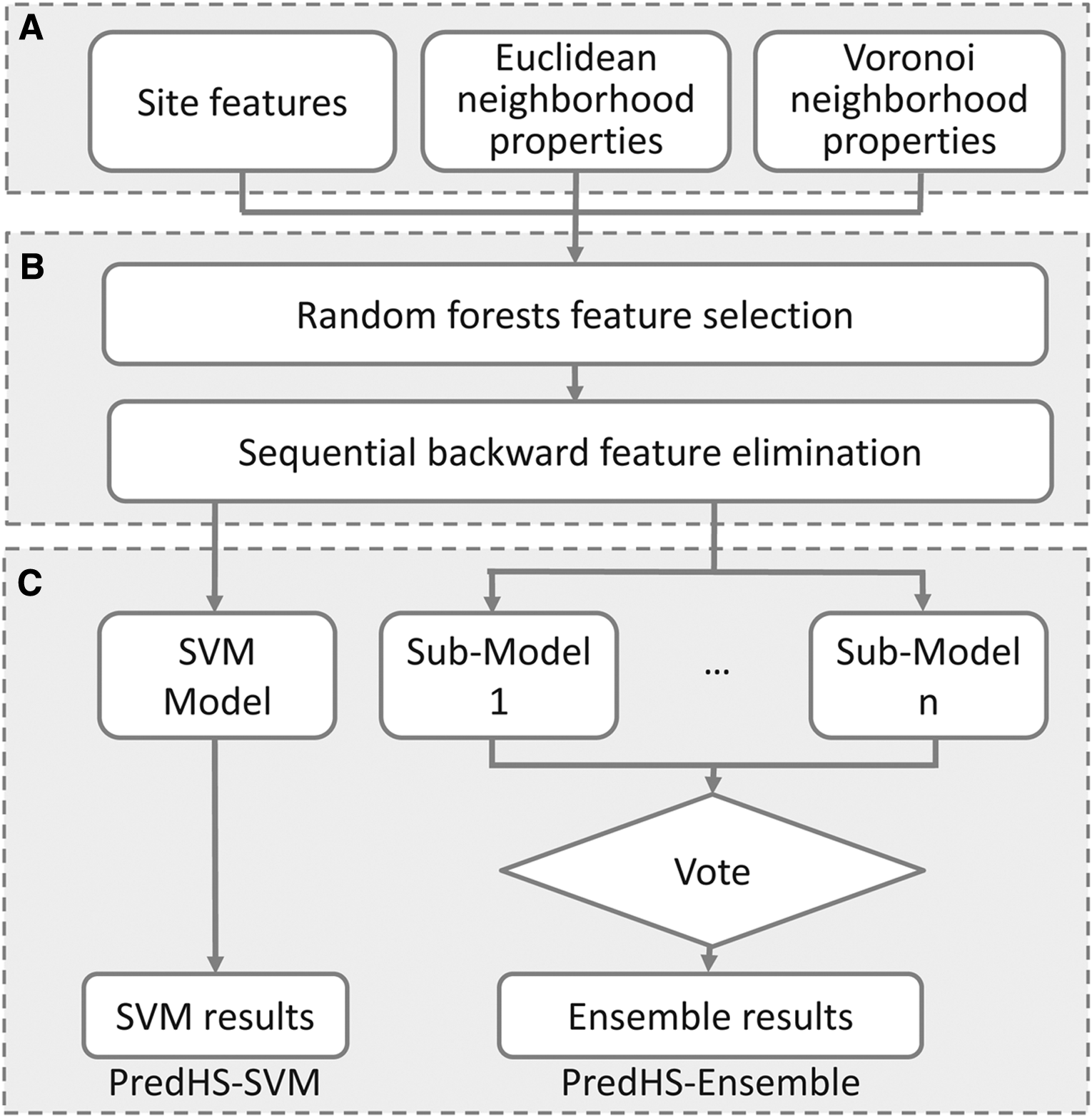
The framework of PredHS. (A) Feature representation: We encode each interface residue using 108 site features, 108 Euclidean neighborhood features, and 108 Voronoi neighborhood features. (B) Two-step feature selection: the first step of feature selection is done by a random forest algorithm, we select the top 77 features with Z-Score larger than 2.5; the second step is performed using a wrapper-based feature selection. Features are evaluated by 10-fold cross-validation with the SVM (support vector machine) algorithm, redundant features are removed by sequential backward elimination. (C) Prediction models: PredHS-SVM and PredHS-Ensemble. For PredHS-Ensemble, an ensemble of n classifiers is built using different subsets, the final result is determined by majority votes among the outputs of the n classifiers.

PredHS-Ensemble uses an ensemble of n classifiers and decision fusion techniques on the training datasets. An asymmetric bootstrap resampling approach is adopted to generate subsets. It performs random sampling with replacement only on the majority class so that its size is equal to the number of minority samples and keeps the entire minority samples in all subsets.

First, the majority class of non–hot spots is undersampled and split into n groups by random sampling with replacement, where each group has the same or similar size as the minority class of interaction sites. After the sampling procedure, we obtain n new datasets from the set of non–hot spots. Each of the new datasets and the set of hot spots are combined into n new training datasets. Then, we train n submodels by using the n new training datasets as input. Each of these classifiers is a support vector machine (SVM). Here the LIBSVM package 2.8 is used with radial basis function (RBF) as the kernel. Finally, a simple majority voting method is adopted in the fusion procedure, and the final result is determined by majority votes among the outputs of the n classifiers.

Algorithm 1:

Two-step feature selection of PredHS

Input:

Given the training set

\documentclass{aastex}\usepackage{amsbsy}\usepackage{amsfonts}\usepackage{amssymb}\usepackage{bm}\usepackage{mathrsfs}\usepackage{pifont}\usepackage{stmaryrd}\usepackage{textcomp}\usepackage{portland, xspace}\usepackage{amsmath, amsxtra}\pagestyle{empty}\DeclareMathSizes{10}{9}{7}{6}\begin{document} $$T = \{ ( x_i , y_i ) \} _{i = 1}^{N} , \ x_i \in {\mathbb S}^n$$ \end{document}

Output:

Initialize

\documentclass{aastex}\usepackage{amsbsy}\usepackage{amsfonts}\usepackage{amssymb}\usepackage{bm}\usepackage{mathrsfs}\usepackage{pifont}\usepackage{stmaryrd}\usepackage{textcomp}\usepackage{portland, xspace}\usepackage{amsmath, amsxtra}\pagestyle{empty}\DeclareMathSizes{10}{9}{7}{6}\begin{document} $${ \rm S} = [ 1 , \ 2 , \ldots { \rm n} ]$$ \end{document}

to the subset of surviving features; ranked feature set

R = [ ];

Train a random forest with features in set S as input variables;

Calculate MDGI Z-Score for each feature in S;

Features with MDGI Z-Score smaller than 2.5 are removed from S;

while S ≠ [ ] do

for each variable i in S, do

Train SVM classifiers on feature set S′, a subset of S exclusive of variable i;

Evaluate the ranking criterion Rc(i) of variable i;

end for

Rank the variable that maximizes Rc;

best = arg max_i Rc;

R = [best R];

Remove the variable best from the set S;

end

Return the ranked feature set R.

3. Results

3.1. Predictive power of structural neighborhood properties

We investigated four types of features—site, sequence, Euclidean, and Voronoi features. The residue features consist of a total of 108 sequence, structural, and energy attributes, a significant portion of which are novel for hot spot identification. The other three types of features (sequence, Euclidean, and Voronoi) are neighborhood properties that describe a residue by summing its neighbors' residue properties. For the sequence features, we include 10 residues upstream and 10 residues downstream of the target residue in the protein sequence as the sequence neighborhood. The Euclidean and Voronoi features are described in detail in Section 2.4.

Four SVM classifiers were trained and tested using the four types of features in Dataset I and 10-fold cross-validation. Their predictive performances are presented in Figure 3. We found that structural neighborhood properties (Euclidean and Voronoi) achieve the best performance, suggesting that structural neighborhood properties are more predictive than site properties in determining hot spots. We also observed that the classifier with linear sequence neighborhood properties is the worst performer, whose area under the ROC curve is significantly smaller than that of the classifier with site features.

FIG. 3.

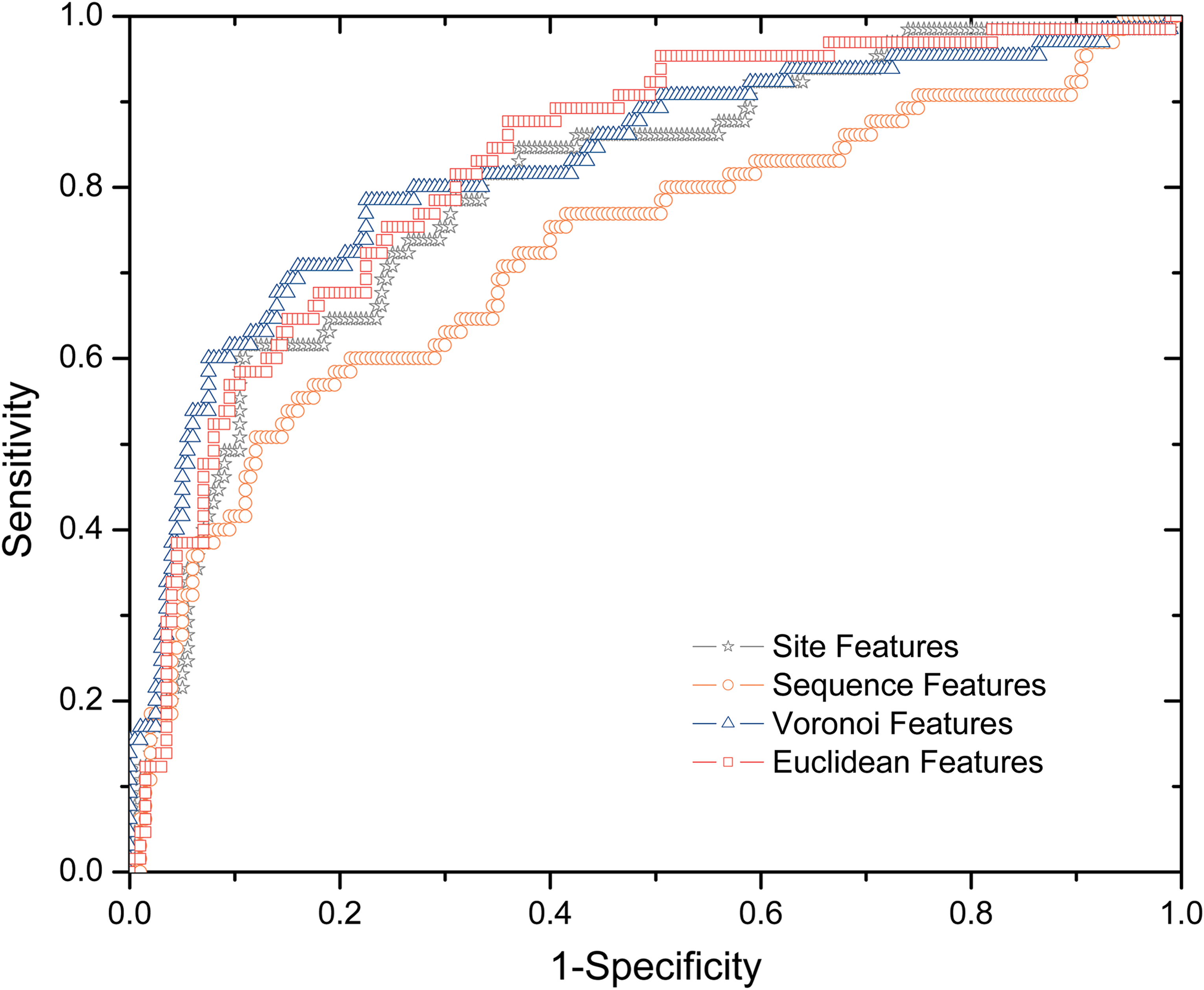
ROC (receiver operating characteristic) curves of classifiers with four types of features (site, sequence, Euclidean, and Voronoi).

3.2. Selection of optimal features

The main goal of this study is to build effective and accurate models to predict hot spots. To this end, identification of a set of informative features is critical for performance boosting and subsequently will enhance our understanding in the molecular basis of hot spots. We combine 324 site, Euclidean, and Voronoi features for further feature selection. The 108 sequence features are not included in the combination since they perform significantly worse in the comparison study of Section 3.1. To assess the feature importance of the 324 features in predicting hot spots, we applied a two-step feature selection method on Dataset I. As a result, a set of 38 optimal features are obtained and listed in Table 1. We found that structural neighborhood properties (Euclidean and Voronoi properties) dominate the top-38 list, suggesting that structural neighborhood properties are more predictive than site properties in determining hot spot residues.

Table 1.

The Top 38 Optimal Features for Hot Spot Prediction Based on the Two-Step Feature Selection Method

Rank	Feature name	Z-Score	Feature type
1	PSSM(Y)	3.057	Site
2	Weighted relative surface burial in Euclidean neighborhood	6.293	Euclidian
3	Relative surface burial	7.055	Site
4	Sidechain energy score in Voronoi neighborhood	3.211	Voronoi
5	Physicochemical properties (polarity) in Euclidean neighborhood	3.153	Euclidian
6	Binary sidechain energy score in Voronoi neighborhood	2.94	Voronoi
7	Weighted conservation score	2.6	Site
8	Weighted PSSM(R) in Voronoi neighborhood	3.39	Voronoi
9	Weighted PSSM(S) in Euclidean neighborhood	4.16	Euclidian
10	Weighted normalized atom contacts in monomer	4.121	Site
11	Weighted binary sidechain energy score in Euclidean neighborhood	3.668	Euclidian
12	Weighted PSSM(R)	4.152	Site
13	Weighted four-body statistical pseudo-potential	3.311	Site
14	Weighted PSSM(E)	2.645	Site
15	Weighted physicochemical properties (propensities)	3.572	Site
16	Weighted Voronoi residue contacts in Euclidean neighborhood	4.614	Euclidian
17	Weighted sidechain energy score in Euclidean neighborhood	2.856	Euclidian
18	Weighted normalized residue contacts in monomer	3.37	Site
19	ConSurf score in Voronoi neighborhood	5.94	Voronoi
20	Residue-interface propensity score in Voronoi neighborhood	2.659	Voronoi
21	Physicochemical properties (polarizability) in Euclidean neighborhood	2.569	Euclidian
22	Binary sidechain energy score in Euclidean neighborhood	6.046	Euclidian
23	Weighted normalized residue contacts in monomer in Euclidean neighborhood	3.627	Euclidian
24	Weighted PSSM(K)	4.124	Site
25	Weighted PSSM(K) in Euclidean neighborhood	2.798	Euclidian
26	Weighted PSSM(K)	3.193	Voronoi
27	Δ pair potential	3.433	Site
28	Weighted Voronoi atom contacts in Euclidean neighborhood	3.198	Euclidian
29	Weighted PSSM(C)	2.574	Site
30	Weighted PSSM(Y)	3.283	Site
31	Weighted topographical index in Euclidean neighborhood	3.523	Euclidian
32	Weighted normalized residue contacts in complex in Euclidean neighborhood	4.204	Euclidian
33	Combined energy score	3.487	Site
34	Relative surface burial in Euclidean neighborhood	5.301	Euclidian
35	Pair potentia in complex in Euclidean neighborhood	2.522	Euclidian
36	Weighted topographical index	2.99	Site
37	Weighted physicochemical properties (polarity) in Euclidean neighborhood	3.024	Euclidian
38	Weighted ConSurf score in Voronoi neighborhood	4.392	Voronoi

The Z-Score is calculated in the first step based on Random Forests.

To quantitatively assess the performance of the two-step feature selection algorithm in PredHS, we compare it with four widely used feature selection methods: random forests, information gain, chi-squared, and F-score. Figure 4 shows the ROC plots of the five feature selection methods based on Dataset I and 10-fold cross-validation. As can be seen from Figure 4, our two-step feature selection algorithm achieves the best performance. The proposed two-step feature selection algorithm, which is a hybrid approach integrating the merits of both filter methods and wrapper methods, can effectively improve the prediction performance with less computational cost and reduce the risk of overfitting.

FIG. 4.

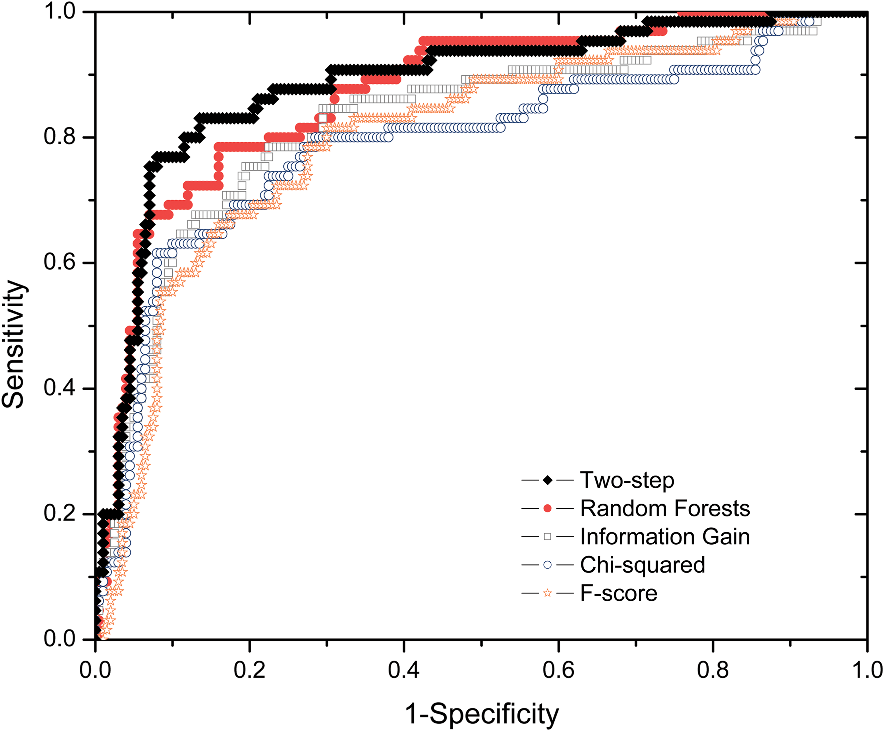
ROC curves of our two-step algorithm and four existing feature selection methods.

3.3. Performance comparison with the state-of-the-art approaches

To evaluate the performance of the proposed PredHS, eight existing hot spot prediction methods, Robetta (Kortemme and Baker, 2002), FOLDEF (Guerois et al., 2002), KFC (Darnell et al., 2007), MINERVA2 (Cho et al., 2009), HotPoint (Tuncbag et al., 2009), APIS (Xia et al., 2010), KFC2a, and KFC2b (Zhu and Mitchell, 2011) are implemented and evaluated on both Dataset I and Dataset II with 10-fold cross-validation. The performance of each model is measured by six metrics: accuracy (Accu), sensitivity (Sen), specificity (Spe), precision (Pre), CC, and F1 score. F1-score is the harmonic mean of the precision and recall (equivalent to sensitivity), which is widely used to handle unbalanced data such as hot spot data.

Table 2 shows the detailed results of comparing our method with the existing methods. On Dataset I, our approach (PredHS-SVM and PredHS-Ensemble) shows dominant advantage over the existing methods in five metrics: accuracy, sensitivity, precision, CC, and F1-score. Only in specificity, FOLDEF and MINERVA2 perform as good as PreHS-SVM; all have the highest specificity value 0.93. Concretely, PredHS-Ensemble predicts the most actual hot spots as hot spots among these methods (with sensitivity = 0.85), while PredHS-SVM identifies the second-most hot spots (with sensitivity = 0.75). Especially, PreHS-Ensemble's sensitivity is 47% higher than that of MINERVA2, which has the highest sensitivity among the existing methods. This suggests that our PredHS model is superior for predicting hot spot residues. Furthermore, PredHS-SVM's CC and F1 score are 25.5% and 19% respectively higher than that of MINERVA2 (still is the best in these two measures among the existing methods). Compared with PredHS-SVM, PredHS-Ensemble is much higher in sensitivity but relatively lower in specificity, however PredHS-Ensemble has much better balance of prediction accuracy between positive examples and negative examples.

Table 2.

Performance Comparison on Dataset I and Dataset II

	Dataset I						Dataset II
Methods	Accu	Sen	Spe	Pre	CC	F1	Accu	Sen	Spe	Pre	CC	F1
PredHS-SVM	0.88	0.75	0.93	0.79	0.69	0.76	0.87	0.86	0.87	0.84	0.74	0.84
PredHS-Ensemble	0.82	0.85	0.81	0.60	0.60	0.69	0.87	0.91	0.84	0.80	0.74	0.85
Robetta	0.80	0.51	0.9	0.62	0.44	0.56	0.77	0.51	0.96	0.89	0.54	0.65
FOLDEF	0.78	0.31	0.93	0.59	0.31	0.40	0.70	0.31	0.98	0.91	0.41	0.46
KFC	0.79	0.55	0.87	0.58	0.43	0.57	0.74	0.55	0.87	0.75	0.45	0.64
MINERVA2	0.84	0.58	0.93	0.72	0.55	0.64	0.81	0.58	0.97	0.93	0.62	0.72
HotPoint	0.72	0.54	0.78	0.44	0.29	0.48	0.73	0.54	0.86	0.73	0.43	0.62
APIS	0.76	0.43	0.87	0.54	0.33	0.46	0.75	0.74	0.75	0.70	0.50	0.71
KFC2a	0.82	0.55	0.91	0.66	0.49	0.59	0.83	0.84	0.82	0.78	0.67	0.80
KFC2b	0.78	0.47	0.88	0.60	0.38	0.51	0.81	0.74	0.86	0.82	0.62	0.75

Six performance measures are used: accuracy (Accu), sensitivity (Sen), specificity (Spe), precision (Pre), CC, and F1 score. The highest values are highlighted in bold.

As for Dataset II, PredHS still performs best in four performance metrics (accuracy, sensitivity, CC, and F1-score). Again, this shows that PreHS can correctly predict more hot spots and has better balance in precision and recall than the existing methods. For almost all compared predictors, results of Dataset II are better than that of Dataset I, this is because Dataset II is a trimmed dataset where residues with ΔΔG between 0.4 and 2.0 are eliminated, which makes the prediction task not so tough.

3.4. Performance evaluation by independent test

We further validate the performance of the proposed model (PredHS-SVM and PredHS-Ensemble) on the independent test dataset. Results of the independent test are presented in Table 3. We can see that our PreHS approach substantially outperforms the existing methods in five performance metrics (accuracy, specificity, precision, CC, and F1 score), only KFC2a has a similar sensitivity value to that of PreHS-Ensemble, that is 0.74, the highest among the 10 compared predictors. Furthermore, the F1-scores of PredHS-SVM and PredHS-Ensemble are 0.68 and 0.68 respectively, while those of the existing methods fall in the range of 0.33–0.64. The findings from the independent test also indicate that the proposed PredHS model performs significantly better than the state-of-the-art approaches.

Table 3.

Performance Comparison on the Independent Test Dataset

Methods	Accu	Sen	Spe	Pre	CC	F1
PredHS-SVM	0.83	0.59	0.93	0.79	0.57	0.68
PredHS-Ensemble	0.79	0.74	0.80	0.63	0.53	0.68
Robetta	0.70	0.33	0.86	0.52	0.23	0.41
FOLDEF	0.68	0.26	0.87	0.48	0.16	0.33
KFC	0.68	0.31	0.85	0.48	0.18	0.38
MINERVA2	0.77	0.46	0.91	0.69	0.42	0.55
HotPoint	0.69	0.59	0.74	0.5	0.31	0.54
APIS	0.71	0.56	0.77	0.52	0.33	0.54
KFC2a	0.74	0.74	0.74	0.56	0.41	0.64
KFC2b	0.79	0.59	0.87	0.68	0.47	0.63

The highest values are highlighted in bold.

3.5. Case study

The protein complex formed by nidogen-1 and perlecan IG3 (PDB code 1GL4) (Kvansakul et al., 2001) was analyzed. The prediction model of PredHS (including PredHS-SVM and PredHS-Ensemble) is highly accurate when compared with the available experimental data, as shown in Figure 5. Five out of 27 interface residues (D427, H429, Y431, E616, and R620) that mediate the interaction between nidogen-1 and perlecan IG3 have been experimentally verified as hot spot residues with ΔΔG ≥ 2.0 kcal/mol (Fig. 5A). Prediction results of PredHS-SVM and PredHS-Ensemble are shown in Figure 5B and C respectively. Four critical residues (D427, H429, Y431, and R620) out of the five experimentally verified hot spots were correctly identified both by PredHS-SVM and PredHS-Ensemble. As expected, PredHS-Ensemble generated more false-positive residues than PredHS-SVM.

FIG. 5.

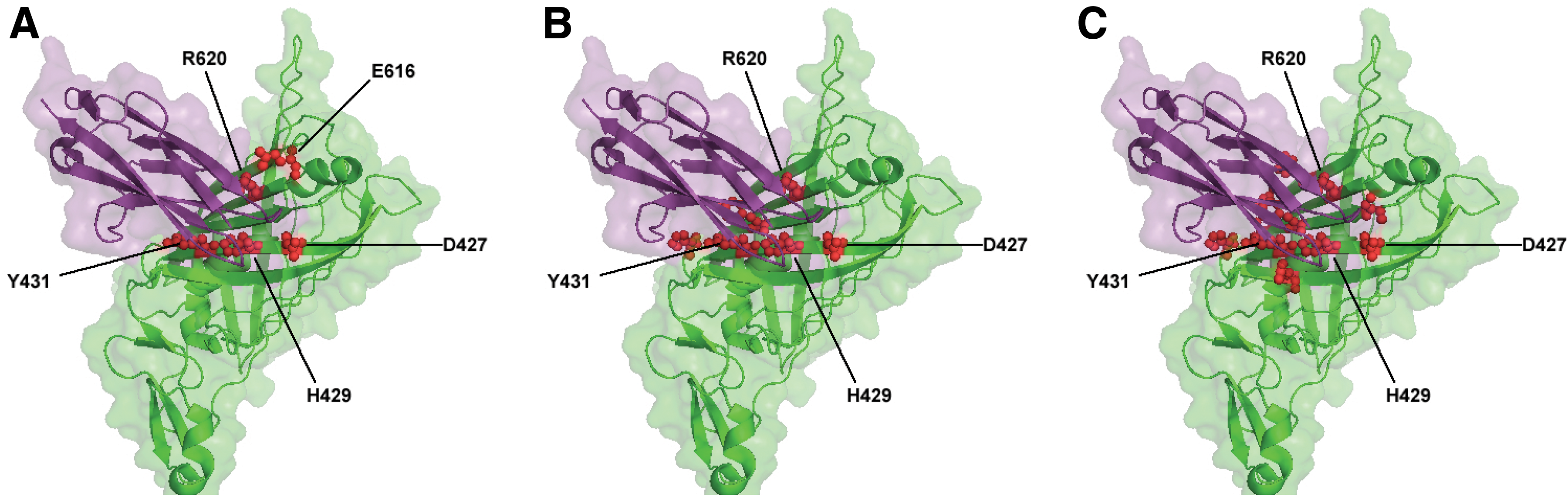
Comparison between experimentally determined hot spot residues (A) and predicted hot spot residues (B and C). Results of (B) and (C) are generated by using PredHS-SVM and PredHS-Ensemble respectively. The green surface represents nidogen-1 (PDB code 1GL4, chain A), while the purple surface denotes perlecan IG3 (PDB code 1GL4, chain B). Residues shown in red are either experimentally determined or predicted as hot spots.

3.6. Web server

A web server interface of our method, named PredHS, is freely available online. Input to the PredHS web server can be a protein complex structure file in PDB format, or a PDB code. Users can select the target protein and its partners and then submit them for prediction. The output contains the predicted result and the predicted confidence, which can be downloaded in text format. Individual predictions can be visualized in the AstexViewer (Hartshorn, 2002). Interface residues are rendered in different colors according to their predicted confidence score.

4. Conclusion

Protein–protein interaction hot spots at the interfaces comprise a small fraction of the interface residues that make a dominant contribution to the free energy of binding. Alanine-scanning mutagenesis experiments to identify hot spot residues are expensive and time-consuming, and computational methods can thus be helpful in suggesting residues for possible experimentation. In this study, we proposed a novel method-PredHS, including PredHS-SVM and PredHS-Ensemble-to predict hot spot residues in protein interfaces. Two key factors are responsible for our success. First, the wide exploitation of heterogeneous information, that is, sequence-based, structure-based, and energetic features, together with two types of structural neighborhoods (Euclidian and Voronoi), provides more important clues for hot spot identification. A total of 324 features, including 108 site properties, 108 Euclidian neighborhood properties, and 108 Voronoi neighborhood properties, have been investigated. Second, our two-step feature selection approach, which combines random forest and a sequential backward elimination, provides an ideal way for selecting an optimal subset of features within a reasonable computational cost. Also, the two-step method can significantly improve the prediction performance and reduce the risk of overfitting.

Our results highlight the advantages of basing hot spot prediction methods on structural neighborhood properties. Compared with other computational hot spot prediction models, PredHS offers significant performance improvement both in terms of precision and recall as well as F1 score that measures the balance between precision and recall. PredHS-Ensemble has the highest sensitivity compared to other methods, but it has a lower specificity than PredHS-SVM. This is because that PredHS-Ensemble incorporates bootstrap resampling techniques and SVM-based fusion classifiers to balance sensitivity and specificity.

As for future work, major existing hot spot prediction methods, including MINERVA2 and KFC2a/b, are considered to be integrated into the PredHS web server to further improve the prediction performance by using Bayesian networks.

Footnotes

Acknowledgments

This work was supported by the China 863 Program under grant no. 2012AA020403 and the National Natural Science Foundation of China under grants nos. 61173118 and 61272380.

Author Disclosure Statement

The authors declare they have no conflicting financial interests.

References

Alberts

B.D.

, Bray

, Lewis

et al. 1989. Molecular Biology of the Cell. Garland, New York.

Assi

S.A.

, Tanaka

, Rabbitts

T.H.

et al. 2009. PCRPi: Presaging critical residues in protein interfaces, a new computational tool to chart hot spots in protein interfaces. Nucleic Acids Res., 38:e86.

Barber

C.B.

, Dobkin

P.D.

, Huhdanpaa

1996. The Quickhull algorithm for convex hulls. ACM Transactions on Mathematical Software, 22:469–483.

Bogan

A.A.

, Thorn

K.S.

1998. Anatomy of hot spots in protein interfaces. J. Mol. Biol., 280:1–9.

Brenke

, Kozakov

, Chuang

et al. 2009. Fragment-based identification of druggable ‘hot spots’ of proteins using Fourier domain correlation techniques. Bioinformatics, 25:621–627.

Chan

C.H.

, Liang

H.K.

, Hsiao

N.W

et al. 2004. Relationship between local structural entropy and protein thermostability. Proteins, 57:684–691.

Cho

, Kim

, Lee

2009. A feature-based approach to modeling protein-protein interaction hot spots. Nucleic Acids Res., 37,8:2672–2687.

Clackson

, Wells

J.A.

1995. A hot spot of binding energy in a hormone-receptor interface. Science, 267:383–386.

Darnell

S.J.

, Page

, Mitchell

J.C.

2007. An automated decision-tree approach to predicting protein interaction hot spots. Proteins, 68:813–823.

10.

DeLano

W.L.

2002. Unraveling hot spots in binding interfaces: progress and challenges. Current Opinion in Structural Biology, 12:14–20.

11.

Fischer

T.B.

, Arunachalam

K.V.

, Bailey

et al. 2003. The binding interface database (BID): a compilation of amino acid hot spots in protein interfaces. Bioinformatics, 19:1453–1454.

12.

Grosdidier

, Fernández-Recio

2008. Identification of hot-spot residues in protein-protein interactions by computational docking. BMC Bioinformatics, 9:447.

13.

Guerois

, Nielsen

J.E.

, Serrano

2002. Predicting changes in the stability of proteins and protein complexes: A study of more than 1000 mutations. J. Mol. Biol., 320:369–387.

14.

Hartshorn

M.J.

2002. AstexViewer: a visualisation aid for structure-based drug design. J. Comput. Aided Mol. Des., 16:871–881.

15.

Huo

, Massova

, Kollman

P.A.

2002. Computational alanine scanning of the 1:1 human growth hormone-receptor complex. J. Comput. Chem, 23:15–27.

16.

Kabsch

, Sander

1983. Dictionary of protein secondary structure: pattern recognition of hydrogen-bonded and geometrical features. Biopolymers, 22:2577–2637.

17.

Kortemme

, Baker

2002. A simple physical model for binding energy hot spots in protein-protein complexes. Proc. Natl. Acad. Sci., 99:14116–14121.

18.

Kvansakul

, Hopf

, Ries

et al. 2001. Structural basis for the high-affinity interaction of nidogen-1 with immunoglobulin-like domain 3 of perlecan. EMBO J, 20:5342–5346.

19.

, Liu

2009. ‘Double water exclusion’: a hypothesis refining the O-ring theory for the hot spots at protein interfaces. Bioinformatics, 25:743–750.

20.

Liang

, Grishin

N.V.

2004. Effective scoring function for protein sequence design. Proteins, 54:271–281.

21.

Liang

, Meroueh

S.O.

, Wang

et al. 2009. Consensus scoring for enriching near-native structures from protein-protein docking decoys. Proteins, 75:397–403.

22.

Liaw

, Wiener

2002. Classification and regression by randomForest. R news, 2:18–22.

23.

Massova

, Kollman

P.A.

1998. Computational alanine scanning to probe protein-protein interactions: A novel approach to evaluate binding free energies. J. Am. Chem. Soc., 120:9401–9409.

24.

Moreira

I.S.

, Fernandes

P.A.

, Ramos

M.J.

2007. Hot spots—A review of the protein-protein interface determinant amino-acid residues. Proteins, 68:803–812.

25.

Ofran

, Rost

2007. Protein-protein interaction hotspots carved into sequences. PLoS Comput Biol., 3:e119.

26.

Thorn

K.S.

, Bogan

A.A.

2001. ASEdb: a database of alanine mutations and their effects on the free energy of binding in protein interactions. Bioinformatics, 17:284–285.

27.

Tuncbag

, Gursoy

, Keskin

2009. Identification of computational hot spots in protein interfaces: combining solvent accessibility and inter-residue potentials improves the accuracy. Bioinformatics, 25:1513–1520.

28.

Tuncbag

, Salman

F.S.

, Keskin

2010. Analysis and network representation of hotspots in protein interfaces using minimum cut trees. Proteins, 78:2283–2294.

29.

Wang

, Liu

Z.P.

, Zhang

X.S.

et al. 2012. Prediction of hot spots in protein interfaces using a random forest model with hybrid features. Protein Engineering, Design & Selection, 25:119–26

30.

Xia

, Zhao

X.M.

, Song

et al. 2010. APIS: accurate prediction of hot spots in protein interfaces by combining protrusion index with solvent accessibility. BMC Bioinformatics, 11:174.

31.

Zhu

, Mitchell

J.C.

2011. KFC2: A knowledge-based hot spot prediction method based on interface solvation, atomic density, and plasticity features. Proteins, 79:2671–2683.

Supplementary Material

Please find the following supplemental material available below.

For Open Access articles published under a Creative Commons License, all supplemental material carries the same license as the article it is associated with.

For non-Open Access articles published, all supplemental material carries a non-exclusive license, and permission requests for re-use of supplemental material or any part of supplemental material shall be sent directly to the copyright owner as specified in the copyright notice associated with the article.

0.00 MB

0.19 MB