Detecting Non-Uniform Clusters in Large-Scale Interaction Graphs

Abstract

Graph clustering becomes difficult as the graph size and complexity increase. In particular, in interaction graphs, the clusters are small and the data on the underlying interaction are not only complex, but also noisy due to the lack of information and experimental errors. The graphs representing such data consist of (possibly overlapping) clusters of non-uniform size with some false positive and false negative links. In this article, we propose a new approach, assuming that clusters in the graphs of protein–protein interaction (PPI) networks resemble corrupted cliques. Therefore, the problem can be reduced to looking for clusters only among nodes of approximately similar degrees. This idea was implemented using a soft version of the Farthest-Point-First (FPF) clustering algorithm with the Jaccard distance function modified to perform on slightly overlapping clusters. The StripClust program developed by us was tested on a synthetic network and on the yeast PPI network.

1. Introduction

Clustering methods in protein—protein interaction (PPI) networks are widely used now as effective tools for identifying functional modules (molecular complexes) in cells, which is one of the important problems in molecular biology. A variety of approaches to such clustering have been proposed in the last decade (see Schaeffer, 2007, for review).

Generally speaking, all algorithms for graph clustering can be classified in two ways: according to their measure for identifying clusters, and according to the method of identifying clusters with a selected measure (see Wang et al., 2010, for review). In one group of algorithms, a particular definition of similarity (i.e., of the distance between the vertices) is used and the clusters are assigned based on the distances. Some examples of the distances are a vector space, such as Euclidean, Manhattan, and cosine (Ochini coefficient), specific graph measures, such as the Jaccard index (used in our approach, which is described below), and connectivity measures. The algorithms of the other group are based on the optimization of the fitness function that reflects the desirable property of the clusters, such as the cluster density (defined as the density of the corresponding subgraphs) or the connectivity of the clusters with the rest of the graph. The choice of the disable properties (measure) for the clusters to be identified depends on the available data and on the corresponding network organization (model). Accordingly, there is a great variety of methods proposed for finding clusters with a selected measure (see reviews by Schaeffer, 2007 and Wang et al., 2010). Below we describe several examples to be further compared with our method.

1) The MCL algorithm (van Dongen, 2000) simulates a flow in the graph by calculating the successive powers of the associated adjacency matrix. Each iteration includes an inflation step to enhance the contrast between the regions of strong and weak flow in the graph. The process converges towards the partition of the graph, with a set of high-flow regions (clusters) separated by boundaries where the flow is absent. The value of the inflation parameter strongly affects the number of clusters. The MCL algorithm performs well on small or sparse graphs, but does not scale well for larger networks.

2) The Girvan–Newman algorithm (Girvan and Newman, 2002) is a divisive clustering technique based on the concept of edge betweenness centrality. The betweenness centrality is the measure of the proportion of the shortest paths between the nodes that pass through a particular link. The algorithm ranks the edges in the graph by their betweenness and removes the edge with the highest score. Then the betweenness is recalculated for the modified graph and the process is repeated. At each step, the set of the connected components of the graph is considered to be the set of resulting clusters. If the desired number of clusters is pre-set, the algorithm comes to a halt when this number of clusters is obtained. The Girvan–Newman algorithm has been shown to perform well on a variety of graph clustering tasks, but its complexity can severely limit its applicability.

3) In theoretical spectral graph methods, eigenvectors are calculated for the Laplacian of the adjacency matrix of a graph. Next, traditional data clustering is performed on the eigenvectors to obtain the clusters of the graph nodes. While these methods produce accurate results, they may be computationally infeasible for large graphs. In some related methods, the link structure is projected into a vector space (instead of using eigenvectors (Dhillon et al., 2004).

4) Quite a few clustering algorithms were developed for the purpose of detecting complexes in biological or social networks. The first step in the method of Molecular Complex Detection (MCODE), which finds densely connected regions, is assigning weight to each vertex that corresponds to its local neighborhood density. Then, the cluster of the top-weighted vertex (the seed vertex) is recursively grown by including in it the vertices whose weight is above a certain given threshold. This threshold corresponds to the percentage of the seed vertex weight, which is defined by the user. MINE, an agglomerative clustering algorithm (Rhrissorrakrai and Gunsalus, 2011), is very similar to MCODE, but it uses a modified vertex weighting strategy and can regulate the measure of network modularity.

The performance of a clustering algorithm with a particular selected measure significantly depends on the correspondence of the proposed network model to the real data. In this work, we consider a protein–protein interaction (PPI) network as a set of functional modules in which each protein interacts with all other proteins of its module and has much less partners for interaction outside the module. In other words, a graph is considered as a set of clique-like subgraphs of different sizes connected by sparse connections. In this representation, the clustering problem consists, actually, in finding all these clique-like subgraphs. Such approach is not new (Spirin and Mirny, 2003); for review of some algorithms for finding clique-like clusters, see Schaeffer, 2007. It was shown that the clique-finding problem is NP-hard (Hastad, 1999). If the cliques are not “complete,” the complexity of the problem increases many-fold (Spirin and Mirny, 2003). Although the PPI networks are very sparse (with respect to the maximal possible number of edges), the problem is complicated by the presence of quite a few false positive and false negative links, which destroy the cliques and result in an increased number of external connections. To overcome this difficulty, several rather complicated heuristic approaches were proposed, for example, the use of the Monte Carlo optimization (Spirin and Mirny, 2003), the superparamagnetic clustering algorithm (Spirin and Mirny, 2003), or the spectral method (Bu et al., 2003). Although functional modules need not always have the clique-like structure, the detection of such clusters can serve as a basis for further improvement of the clustering.

In this article, we describe a new approach to finding clique-like clusters in PPI networks. The proposed algorithm, being very fast, simple, and robust, allows finding clusters of different size. In short, the underlying approach consists in reducing the problem to looking for clusters only among the nodes of similar degrees, along with applying the Farthest-Point-First (FPF) clustering algorithm (Gonzalez, 1985) with the Jaccard distance function (Hennig and Hausdorf, 2006). The optimal number of clusters is determined by using the elbow criterion (Goutte et al., 1999).

2. Methods

2.1. k-core decomposition

Let G = (V, E) be a graph of |V| = n vertices and |E| = e edges. Then,

1. Subgraph H of G induced by set \documentclass{aastex}\usepackage{amsbsy}\usepackage{amsfonts}\usepackage{amssymb}\usepackage{bm}\usepackage{mathrsfs}\usepackage{pifont}\usepackage{stmaryrd}\usepackage{textcomp}\usepackage{portland, xspace}\usepackage{amsmath, amsxtra}\pagestyle{empty}\DeclareMathSizes{10}{9}{7}{6}\begin{document} $${ \rm C} \subseteq { \rm V}$$ \end{document} is a k-core if and only if the degree of each node \documentclass{aastex}\usepackage{amsbsy}\usepackage{amsfonts}\usepackage{amssymb}\usepackage{bm}\usepackage{mathrsfs}\usepackage{pifont}\usepackage{stmaryrd}\usepackage{textcomp}\usepackage{portland, xspace}\usepackage{amsmath, amsxtra}\pagestyle{empty}\DeclareMathSizes{10}{9}{7}{6}\begin{document} $${ \rm v} \in { \rm C}$$ \end{document} induced in H is greater or equal to k and H is the maximum subgraph of such type.

2. Vertex i has shell-index k if it belongs to the k-core, but not to the (k + 1) core.

3. k-shell S_k is composed of all the vertices with shell index k.

Thus a k-core is a combination of all shells S_c with c ≥k. It can be evaluated by recursively removing all vertices of degrees less than k, the minimum degree of all vertices in the remaining graph is k. Note that this process is not equivalent to pruning vertices of a certain degree. For example, a vertex of high degree connected to numerous first- degree vertices and connected to the rest of the graph only by a single edge belongs only to the first shell. An example of the k-core decomposition is shown in Figure 1.

FIG. 1.

Shell indices.

2.2. Distance measure

For each node v \documentclass{aastex}\usepackage{amsbsy}\usepackage{amsfonts}\usepackage{amssymb}\usepackage{bm}\usepackage{mathrsfs}\usepackage{pifont}\usepackage{stmaryrd}\usepackage{textcomp}\usepackage{portland, xspace}\usepackage{amsmath, amsxtra}\pagestyle{empty}\DeclareMathSizes{10}{9}{7}{6}\begin{document} $$\in$$ \end{document} V, let N[v] be the closest neighbourhood of v (containing v and all its adjacent neighbours) (i.e., N[v] = v U {u \documentclass{aastex}\usepackage{amsbsy}\usepackage{amsfonts}\usepackage{amssymb}\usepackage{bm}\usepackage{mathrsfs}\usepackage{pifont}\usepackage{stmaryrd}\usepackage{textcomp}\usepackage{portland, xspace}\usepackage{amsmath, amsxtra}\pagestyle{empty}\DeclareMathSizes{10}{9}{7}{6}\begin{document} $$\in$$ \end{document} V | (u; v) \documentclass{aastex}\usepackage{amsbsy}\usepackage{amsfonts}\usepackage{amssymb}\usepackage{bm}\usepackage{mathrsfs}\usepackage{pifont}\usepackage{stmaryrd}\usepackage{textcomp}\usepackage{portland, xspace}\usepackage{amsmath, amsxtra}\pagestyle{empty}\DeclareMathSizes{10}{9}{7}{6}\begin{document} $$\in$$ \end{document} E}). Note that for each node v, N[v] can be represented by the v^th column of matrix A + I, where A is the graph adjacency matrix and I is the identity matrix. Let p^v = [A + I]^v denotes an n-dimensional point and the size of N[v] is the sum of the elements in p^v. Thus, using vector representation of the closest neighbourhoods of graph nodes, we have obtained embedding of the nodes in the n-dimensional space.

In the context of social networks, two actors are considered to be structurally equivalent if they are connected and share exactly the same contacts. Note that in the corresponding graph, nodes v and u are structurally equivalent if and only if N[v] = N[u]. Based on the idea of structural equivalence in social networks, the Jaccard structural dissimilarity function, denoted jsd(u; v), between nodes v and u defines the Jaccard distance between N[v] and N[u] as: \documentclass{aastex}\usepackage{amsbsy}\usepackage{amsfonts}\usepackage{amssymb}\usepackage{bm}\usepackage{mathrsfs}\usepackage{pifont}\usepackage{stmaryrd}\usepackage{textcomp}\usepackage{portland, xspace}\usepackage{amsmath, amsxtra}\pagestyle{empty}\DeclareMathSizes{10}{9}{7}{6}\begin{document} \begin{align*}{ \rm jsd} ( { \rm u; v} ) = 1 - \mid ( { \rm N} [ { \rm u} ] \cap { \rm N} [ { \rm v} ] ) \mid / \mid ( { \rm N} [ { \rm u} ] \cup [ { \rm N} [ { \rm v} ] ) \mid . \tag{{\rm Eq}.1}\end{align*} \end{document}

It should be pointed out that the function defined above is a proper metric distance and satisfies the triangle inequality. This function can be easily calculated using the Boolean operations on p^v and p^u. Note that nodes v and u are structurally equivalent if and only if jsd(u; v) = 0 and that for every two nodes u and v, 0 ≤ jsd(u; v) ≤ 1. If we consider the graph shown in Figure 2, it is reasonable to assume that the edge connecting nodes v5 and v6 is false positive. Therefore, a proper distance function should result in a relatively large distance between these nodes. Note that simple hop distance is not appropriate in this case, since a false positive edge results in a small false hop distance between each two nodes belonging to different clusters. However, in the case of our distance function, jsd(v5; v6) = 1 - 1/9 = 8/9. On the other hand, the nonexisting edge between v1 and v4 appears to be false negative, so a good distance function should result in a small distance between these two nodes. A simple hop distance equals to 2 hops, which is larger than the hop distance between v5 and v6. With the Jaccard dissimilarity function, we obtain jsd(v1; v4) = 1 - 3/5 = 2/5.

FIG. 2.

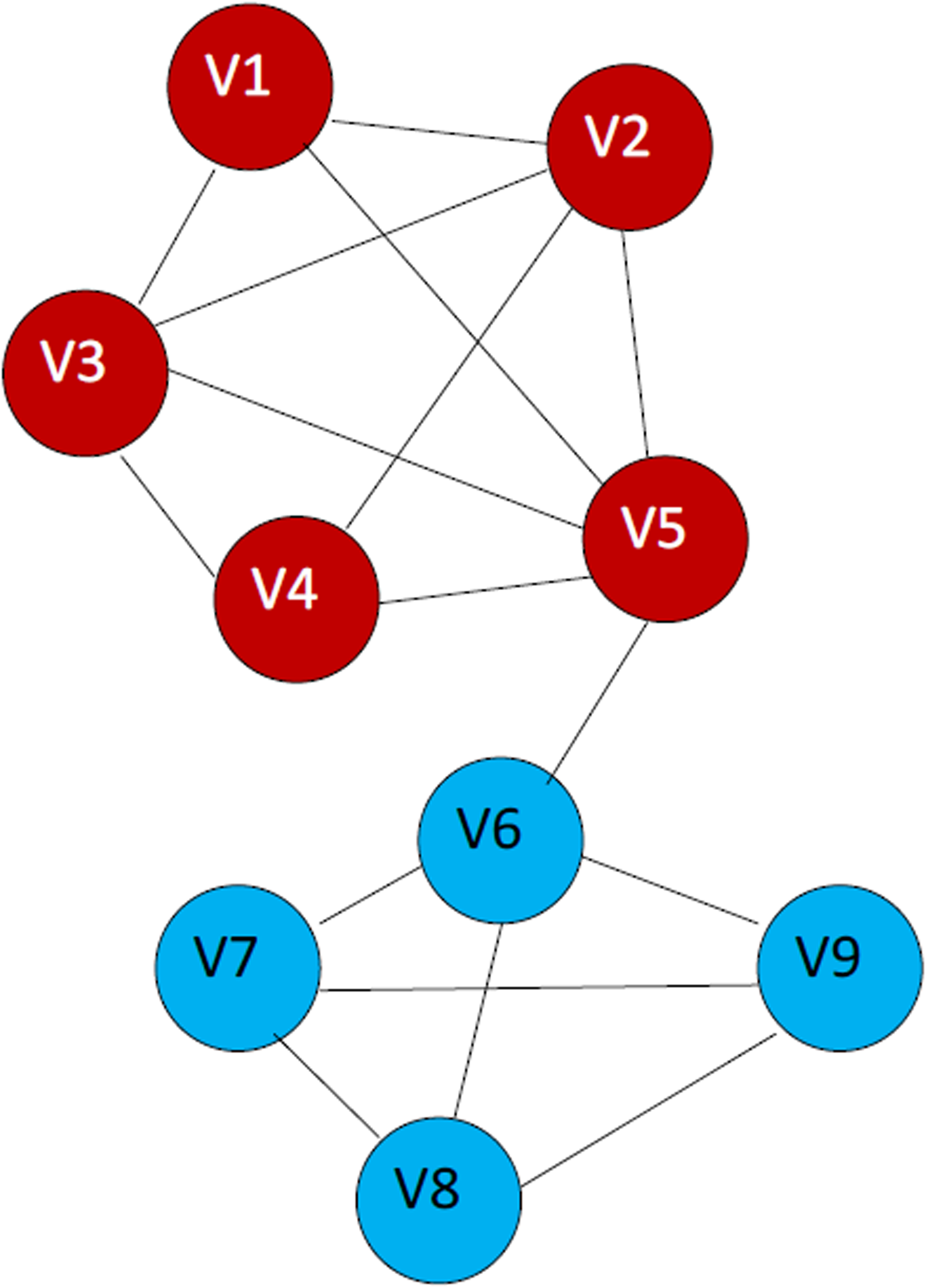
Example of calculation of the distances.

2.3. The Farthest-Point-First method

The FPF algorithm (Gonzalez, 1985) performs clustering over a given set of points by finding the solution of the k-centre problem defined as follow: Given set of points P on metric space M, distance function d satisfying the triangle inequality, and integer k, a k-centre set is subset C of P such that |C| = k. The k-centre problem consists in finding the k-centre set minimizing the maximum distance between each point \documentclass{aastex}\usepackage{amsbsy}\usepackage{amsfonts}\usepackage{amssymb}\usepackage{bm}\usepackage{mathrsfs}\usepackage{pifont}\usepackage{stmaryrd}\usepackage{textcomp}\usepackage{portland, xspace}\usepackage{amsmath, amsxtra}\pagestyle{empty}\DeclareMathSizes{10}{9}{7}{6}\begin{document} $$p \in P$$ \end{document} . and its nearest centre in C, that is, minimizing the target function, \documentclass{aastex}\usepackage{amsbsy}\usepackage{amsfonts}\usepackage{amssymb}\usepackage{bm}\usepackage{mathrsfs}\usepackage{pifont}\usepackage{stmaryrd}\usepackage{textcomp}\usepackage{portland, xspace}\usepackage{amsmath, amsxtra}\pagestyle{empty}\DeclareMathSizes{10}{9}{7}{6}\begin{document} $$max_{p \in p} min_{c \in c}d ( p , c )$$ \end{document} . The constant approximation ratio for this problem obtained using the FPF approximation algorithm is 2. The FPF algorithm is based on the greedy approach, which means that it increasingly computes the sets of points (clusters) \documentclass{aastex}\usepackage{amsbsy}\usepackage{amsfonts}\usepackage{amssymb}\usepackage{bm}\usepackage{mathrsfs}\usepackage{pifont}\usepackage{stmaryrd}\usepackage{textcomp}\usepackage{portland, xspace}\usepackage{amsmath, amsxtra}\pagestyle{empty}\DeclareMathSizes{10}{9}{7}{6}\begin{document} $$C_1 , C_2 , \ldots, C_k$$ \end{document} . Set C₁ contains only one randomly chosen point \documentclass{aastex}\usepackage{amsbsy}\usepackage{amsfonts}\usepackage{amssymb}\usepackage{bm}\usepackage{mathrsfs}\usepackage{pifont}\usepackage{stmaryrd}\usepackage{textcomp}\usepackage{portland, xspace}\usepackage{amsmath, amsxtra}\pagestyle{empty}\DeclareMathSizes{10}{9}{7}{6}\begin{document} $$c_1 \in P$$ \end{document} , while the rest of points in P are assigned to c₁. In other words, initially, centre(p) = c₁ for each point \documentclass{aastex}\usepackage{amsbsy}\usepackage{amsfonts}\usepackage{amssymb}\usepackage{bm}\usepackage{mathrsfs}\usepackage{pifont}\usepackage{stmaryrd}\usepackage{textcomp}\usepackage{portland, xspace}\usepackage{amsmath, amsxtra}\pagestyle{empty}\DeclareMathSizes{10}{9}{7}{6}\begin{document} $$p \in P$$ \end{document} . Prior to each iteration i, (1 < i < k), the set of centres and the assignment of points in P to the centres have already been computed. A new centre is added as follows:

1. determine point \documentclass{aastex}\usepackage{amsbsy}\usepackage{amsfonts}\usepackage{amssymb}\usepackage{bm}\usepackage{mathrsfs}\usepackage{pifont}\usepackage{stmaryrd}\usepackage{textcomp}\usepackage{portland, xspace}\usepackage{amsmath, amsxtra}\pagestyle{empty}\DeclareMathSizes{10}{9}{7}{6}\begin{document} $$p \in P$$ \end{document} that is the farthest from its currently assigned centre centre(p), i.e., point p that satisfies the maximal value max_ped(d(p, center (p)), and set c_i+1 = p;

2. for each point \documentclass{aastex}\usepackage{amsbsy}\usepackage{amsfonts}\usepackage{amssymb}\usepackage{bm}\usepackage{mathrsfs}\usepackage{pifont}\usepackage{stmaryrd}\usepackage{textcomp}\usepackage{portland, xspace}\usepackage{amsmath, amsxtra}\pagestyle{empty}\DeclareMathSizes{10}{9}{7}{6}\begin{document} $$p \in P$$ \end{document} if d(p, centre(p)) > d(p, c_i+1),

i.e., if the new centre is closer to p than its assigned centre, then set centre(p) = c_i+1.

Note that each iteration has complexity O(n) and calculation of a k-centre is O(kn). The computed k-centre set naturally results in the clustering of P, namely, \documentclass{aastex}\usepackage{amsbsy}\usepackage{amsfonts}\usepackage{amssymb}\usepackage{bm}\usepackage{mathrsfs}\usepackage{pifont}\usepackage{stmaryrd}\usepackage{textcomp}\usepackage{portland, xspace}\usepackage{amsmath, amsxtra}\pagestyle{empty}\DeclareMathSizes{10}{9}{7}{6}\begin{document} $$C_j = \{ p \in P \mid center ( p ) = c_j \} $$ \end{document} for each \documentclass{aastex}\usepackage{amsbsy}\usepackage{amsfonts}\usepackage{amssymb}\usepackage{bm}\usepackage{mathrsfs}\usepackage{pifont}\usepackage{stmaryrd}\usepackage{textcomp}\usepackage{portland, xspace}\usepackage{amsmath, amsxtra}\pagestyle{empty}\DeclareMathSizes{10}{9}{7}{6}\begin{document} $$j = 1 , \ldots , k$$ \end{document} . In other words, the j^th cluster consists of all points assigned to the j^th centre.

2.4. The elbow criterion

The FPF algorithm described above requires the input of the number of clusters k. To find this number, we used the elbow criterion. At the elbow point, certain function f reflecting the clustering quality changes the fastest with the number of clusters. This point can be defined as the point of the maximum second derivative of quality function f. For the case of a discrete number of clusters, the second derivative can be obtain by the central difference approximation: f”(k) ≈ f(k - 1) + f(k + 1) - 2f(k).

In this work, we chose quality function f to be the target optimization function, namely, the maximal distance between a point and the corresponding assigned centre. Thus we had to search for the number of clusters k where the central difference f(k – 1) + f(k + 1) - 2f(k) was maximal, which was much easier since the target optimization function f had already been calculated for each execution of the FPF algorithm.

2.5. Outline of the algorithm

The stages of the algorithm proposed in this work are described below.

1. First, divide the nodes into several strips. It is done in one of the following ways:

(a) compute the k-core decomposition of graph G(V; E) and use each shell of the decomposition as a strip;

(b) decompose the sorted array of degrees into several strips, for example, assign all nodes of degrees 2^N ≤ d < 2^N+1 to the N^th strip.

2. Express each node that belongs to the first strip (of small degrees) as a point in the n-dimensional space with the Jaccard structural dissimilarity metric. Then use the FPF algorithm to perform clustering of these points.

3. The nodes assigned to singleton clusters are considered to be unclustered and are passed to the next, higher-degree strip. Add the proper (nonsingleton) clusters to the global clustering.

4. To deal with the nodes that belong several clusters, calculate the affinity of all nodes to each of the added clusters (i.e., for each node count the number of its neighbours in the cluster divided by the total number of neighbors). If the affinity is higher than 1/3, add the node to the cluster.

5. Continue with step 2 to perform clustering of the nodes in the higher-degree strip along with the nodes of the previous strip that were left unclustered.

6. Continue until reaching the inner strip and return the global clustering.

Three procedures of the algorithm are summarized in the pseudo code given in Figure 3.

FIG. 3.

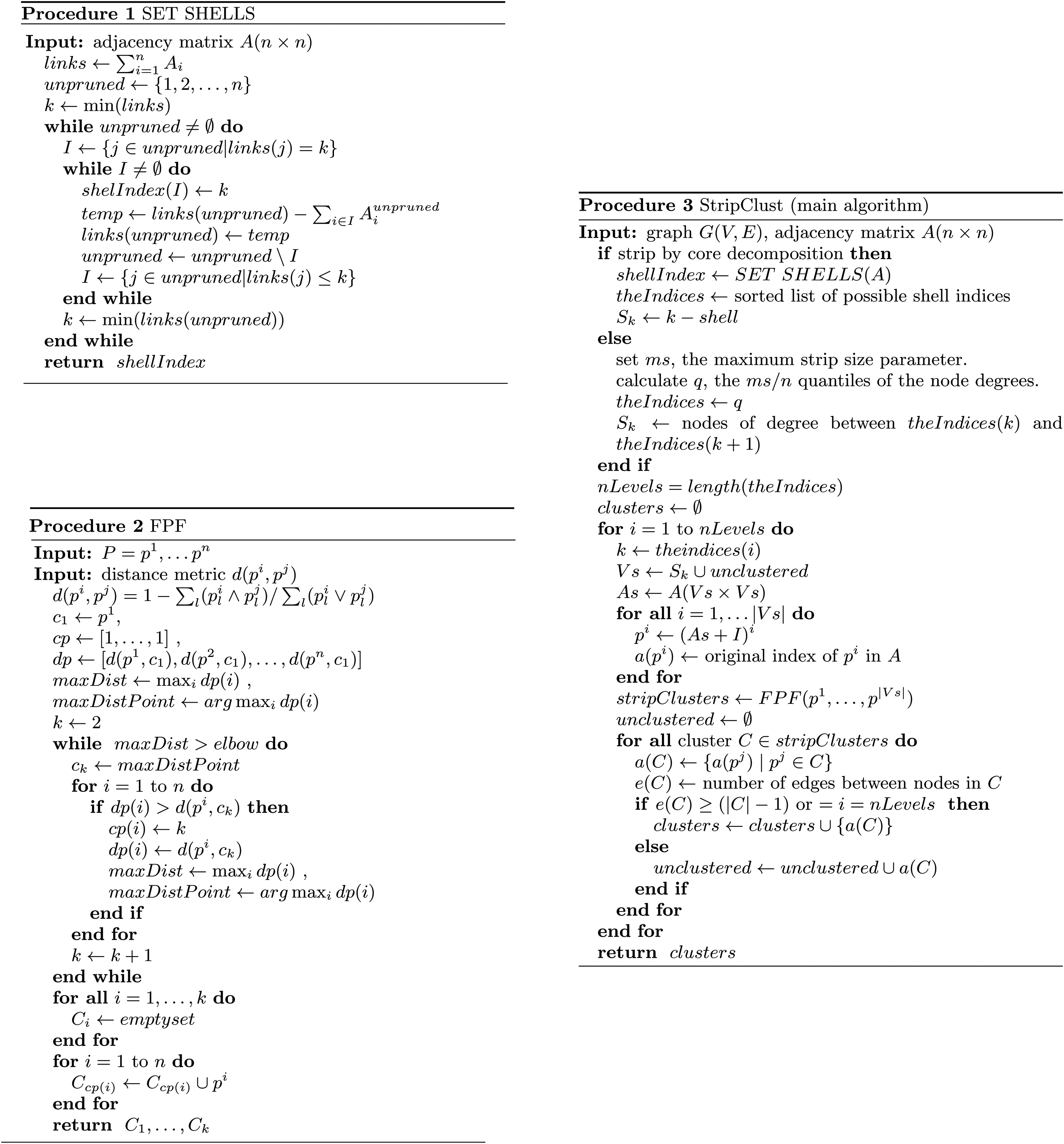
Pseudo code of the main procedures of the algorithm.

2.6. Generation of synthetic networks

We used synthetic networks constructed as proposed in (Brandes et al., 2003; Maier et al., 2011). A set of N nodes was divided into k subsets (clusters), the cluster sizes being drawn using a probability function. Each pair of nodes from the same cluster is related to certain probability, p_in, whereas each pair of nodes from different clusters is related to some other probability, p_out. To simulate the cluster distribution observed in PPNs/PPI networks, the clusters were divided into two groups: small-size and large-size clusters (containing about 10 and 90% of the total number of nodes, respectively).

3. Results

3.1. Algorithm description

Consider an “ideal” graph, composed of various size non-overlapping cliques, with a few connections between the cliques. Let us define the distances between the nodes according to the rule: “the more the number of common neighbors, the less the distance.” Such distance function is called the Jaccard structural dissimilarity function (Hennig and Hausdorf, 2006), see “Methods”: \documentclass{aastex}\usepackage{amsbsy}\usepackage{amsfonts}\usepackage{amssymb}\usepackage{bm}\usepackage{mathrsfs}\usepackage{pifont}\usepackage{stmaryrd}\usepackage{textcomp}\usepackage{portland, xspace}\usepackage{amsmath, amsxtra}\pagestyle{empty}\DeclareMathSizes{10}{9}{7}{6}\begin{document} \begin{align*}{ \rm jsd} ( { \rm u; v} ) = 1 - ( { \rm N} [ { \rm u} ] \cap { \rm N} [ { \rm v} ] ) / ( { \rm N} [ { \rm u} ] \cup { \rm N} [ { \rm v} ] )\end{align*} \end{document}

Obviously, the above definition implies that all distances inside the cliques are much smaller than all the “external” distances. This distance distribution allows easy detection of clusters by the FPF algorithm (Gonzalez, 1985), see “Methods”. At every step, this algorithm adds a new cluster with the center at the point of the maximal distance from all other cluster centers. Since in our “ideal” graph, for all clusters, all the “internal” distances are much smaller than the “external” ones, this algorithm first identifies all cliques as clusters and only thereafter starts dividing the cliques into smaller clusters.

Since the exact number of cliques is usually a priori unknown, it can be determined using the elbow criterion (Goutte et al., 1999), see “Methods”. According to this criterion, the number of clusters is chosen in such a way that the addition of another cluster would not result in a significantly improved partition. The elbow point is the point at which the clustering measure function changes the fastest with the number of clusters. The objective function of the clustering measure was selected to be the sum of the distances of the most distant point from the center of the corresponding cluster. Indeed, if a new cluster is formed by the bisection of a clique, its influence on the objective function is much smaller as compared to the case of dividing two cliques into two clusters.

The algorithm described above appears to be very efficient for ideal graphs. Moreover, even if the cliques are not “good” enough, the algorithm appears to work well once all the Jaccard distances in the clusters are significantly smaller than the external distances. The problems arise when a great number of “additional” vertexes (not related to the cliques) exist in the graph. Such orphan vertexes could be chosen as cluster centres in the FPF algorithm, which would greatly complicate the subsequent identification of cliques and the application of the elbow criterion for determining the number of clusters. To overcome this obstacle, we have proposed a simple method of dividing the initial graph into a set of subgraphs, which are much closer to “ideal” ones. The idea is based on the obvious fact that all nodes that belong to the same clique have similar degrees. Thus, an extracted subgraph which is composed of vertexes of similar degrees will contain all cliques of the corresponding size, while the number of “non-clique” vertexes in it will be much less. We have suggested two different methods of decomposing a graph into several degree-based strips (see “Methods”). The first method employs core-decomposition of the graph. In the second method, the strip size is fixed and the sorted array of degrees is partitioned. See also the outline of the algorithm in “Methods”.

3.2. Application to synthetic network

Initially, the StripClust program, based on the described above algorithm, was tested for detecting original clusters in model networks, generated as described in “Methods.” In addition to the number of detected clustered, the quality of predicting the clusters was also measured. The latter quality was evaluated as the number of correctly predicted external and internal cluster edges, which affect the graph modularity. An example of clustering a synthetic network using the StripClust program is demonstrated in Figure 4. The network consists of 10 large and 10 small clusters (see “Methods”) with p_in = 0.9 and p_out = 0.01. The data presented in Figure 4 show that the elbow point (only the second derivative is shown) exactly corresponds to the number of clusters both for the low-degree and the high-degree nodes. Just at these points all external and internal edges are precisely predicted. It should be noted that, in many cases, our algorithm could accurately predict the initial clustering, in contrast to other executed clustering algorithms (as implemented in the Cluster-maker plug-in in Cytoscape (Morris et al., 2011)). Cluster detection by different algorithms is compared in Table 1 for a model network containing 5 large and 5 small clusters (p_in = 0.9 and p_out = 0.01). Visualization of the initial and the detected clusters is shown in Figure 5. Note that the MCL algorithm can also detect all original clusters in the case of small networks.

FIG. 4.

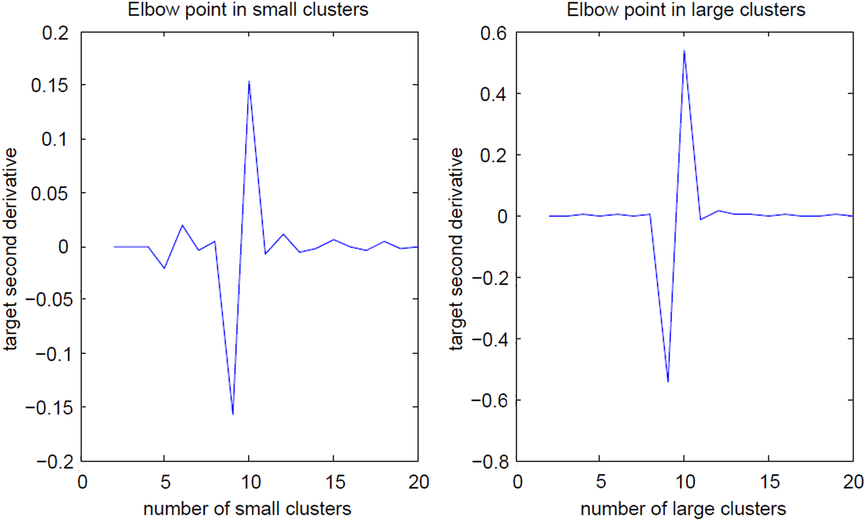
Elbow point. The model network consists of 10 large and 10 small clusters with p_in = 0.9 and p_out = 0.01. The elbow point calculated for the second derivative exactly corresponds to the number of clusters both for the low-degree and the high-degree nodes.

FIG. 5.

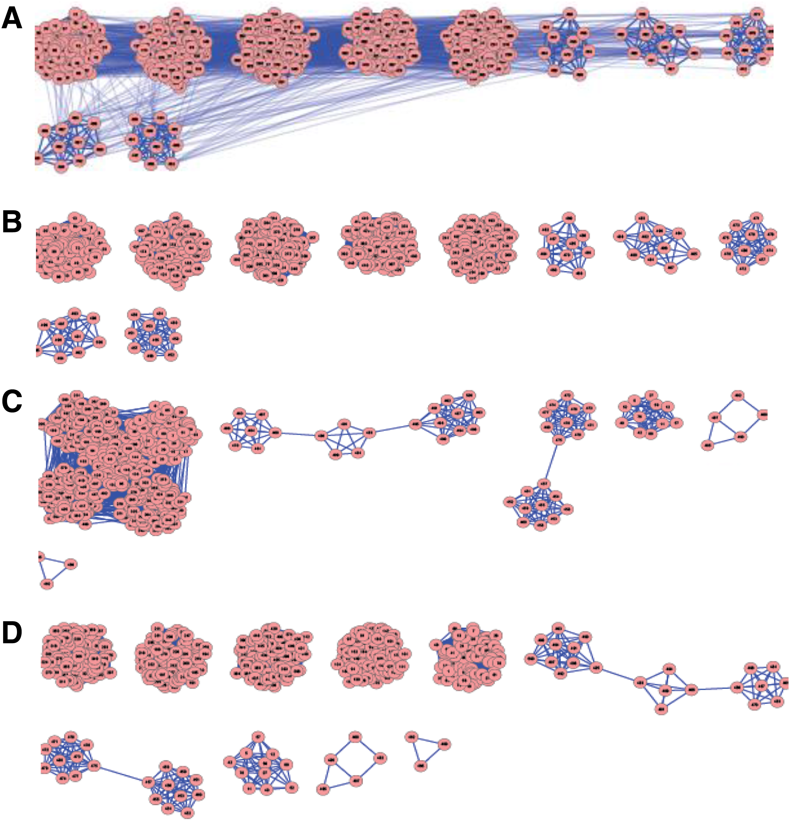
Comparison cluster prediction by different algorithms for model network. The model network consists of 5 large and 5 small clusters (A) is clustered by different approaches: (B) ShellsClust and MCL—100% prediction; (C) Mcode; (D) Girvan and Newman algorithms.

Table 1.

Synthetic Network Results

Results	Mcode	Girvan-Newman	Spectral	MCL	StripClust
Number of clusters	9	10	1	10	10
Min cluster size	3	3	500	10	10
Max cluster size	412	90	500	90	90
Modularity	0.03	0.74	0	0.73	0.73
Intra-cluster prediction	No	No	Yes	Yes	Yes
Inter-cluster prediction	No	No	No	Yes	Yes

3.3. Application to yeast PPI network

The StripClust algorithm was also tested on real-life data, namely, on the yeast PPI network obtained from BioGRID (Stark et al., 2011). The network consists of 6107 different proteins and 183,552 interactions. The results obtained here were compared with the CYC2008 database of known yeast protein complexes (Aranda et al., 2010). This dataset consists of 408 manually curated complexes supplemented by small-scale experiments from the literature (Song and Singh, 2009). For each known group or complex G_i and detected cluster C_j, the Jaccard index and the Precision-Recall (PR) value were calculated: \documentclass{aastex}\usepackage{amsbsy}\usepackage{amsfonts}\usepackage{amssymb}\usepackage{bm}\usepackage{mathrsfs}\usepackage{pifont}\usepackage{stmaryrd}\usepackage{textcomp}\usepackage{portland, xspace}\usepackage{amsmath, amsxtra}\pagestyle{empty}\DeclareMathSizes{10}{9}{7}{6}\begin{document} \begin{align*}{ \rm Jac}_{{ \rm ij}} = ( { \rm G}_{ \rm i} \cap { \rm C_j} ) / ( { \rm G}_{ \rm i} \cup { \rm C}_{ \rm j} ) ; \tag{{\rm Eq}. 2}\end{align*} \end{document} \documentclass{aastex}\usepackage{amsbsy}\usepackage{amsfonts}\usepackage{amssymb}\usepackage{bm}\usepackage{mathrsfs}\usepackage{pifont}\usepackage{stmaryrd}\usepackage{textcomp}\usepackage{portland, xspace}\usepackage{amsmath, amsxtra}\pagestyle{empty}\DeclareMathSizes{10}{9}{7}{6}\begin{document} \begin{align*}{ \rm PR}_{{ \rm ij}} = ( { \rm G}_{ \rm i} \cap { \rm C_j} ) ( { \rm G_j} \cap { \rm C_i} ) / ( \mid { \rm C_j} \mid \ \mid { \rm G_i} \mid ) . \tag{{\rm Eq}. 3}\end{align*} \end{document}

For both of these scores, complex-wise and cluster-wise mapping (Song and Singh, 2009) was carried out. The comparison of the mapping scores obtained using our StripClust algorithm with those obtained with the MCODE, MINE, and MCL algorithms is shown Figure 6. It can be seen that the StripClust algorithm provides the best correspondence of the detected clusters to the known protein complexes and groups.

FIG. 6.

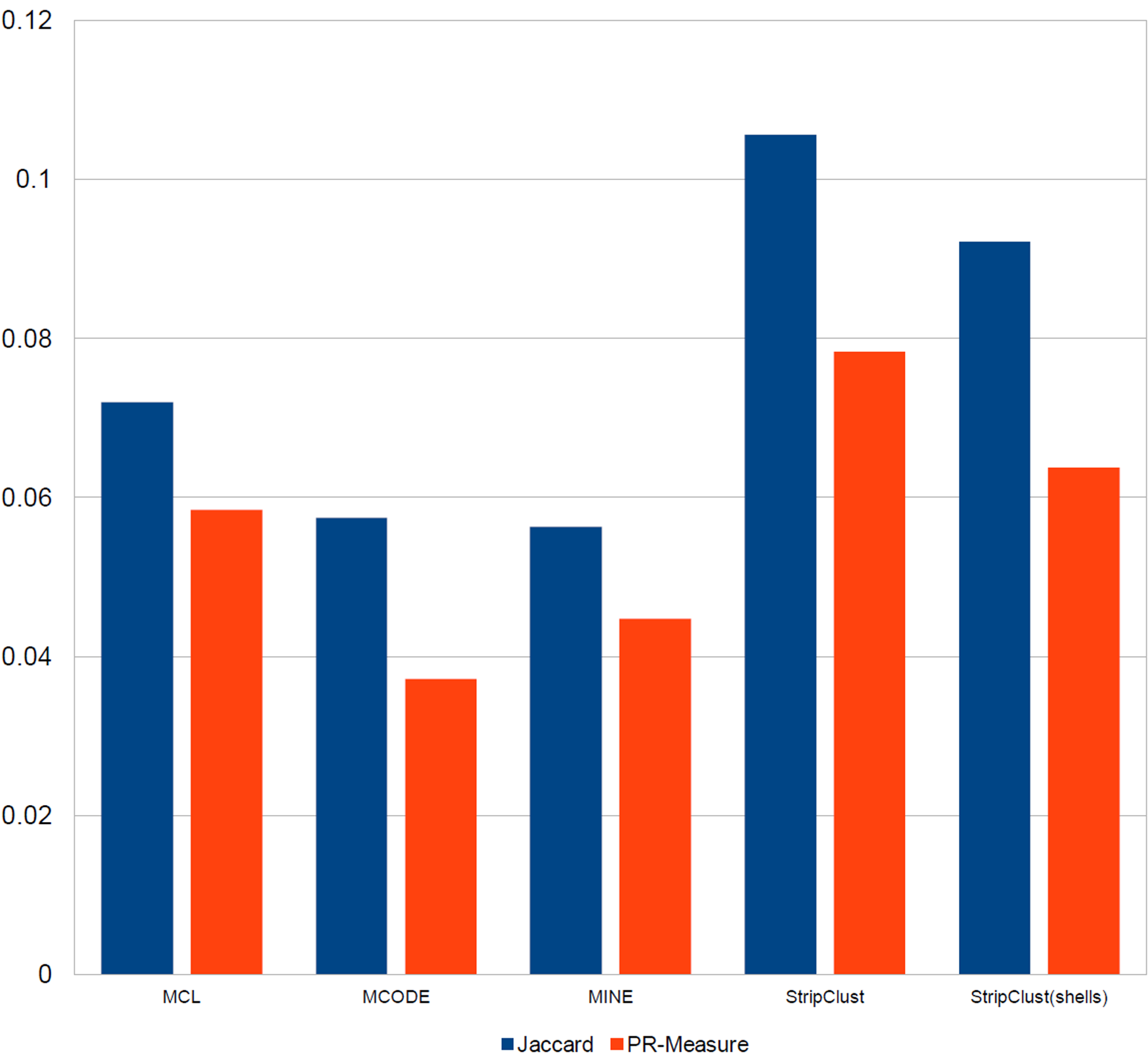
Comparison cluster prediction by different algorithms for yeast PPI network. The network consists of 6107 different proteins and 183,552 interactions. The results of clustering are compared with the CYC2008 database of known yeast protein complexes containing 408 manually curated complexes supplemented by small-scale experiments from the literature (Song and Singh, 2009). For each known group or complex G_i and detected cluster C_j, the Jaccard index and the Precision-Recall (PR) value were calculated.

We have found that the best prediction for this network was obtained using the strips selected according to the node degrees, without using core decomposition (data not shown). However, the quality of the results depends on the strip size parameter (1000 in this experiment, see “Methods”).

Discussion

From the results described above, it follows that the proposed method, in spite of its simplicity, can be effectively used for detecting protein complexes in PPI networks. Clearly, the applicability of this method is limited by specific features of the network, namely, the clusters being clique-like (i.e., most of the cluster nodes should be connected to each other) and the degree of “non-clustered” nodes being different from that of the nodes (at least, most of the nodes) in clusters. However, a very good scalability of the method (which is due to using the fast FPF algorithm and dividing the task into several independent strips) makes it possible to use the method for a wide range of networks to perform efficient simplified pre-calculation before applying more complicated and less scalable clustering approaches, such as spectral clustering. Another way of extending the applicability of the method is refinement of the detected clusters, for example, as it is proposed in Dhillon et al., (2007). Alternatively, the method can be improved by performing the operations in an inverse order, namely, by conversion of a nonappropriate graph into a form suitable for our method. For example, it can be a procedure similar to successive power and inflation steps used in the MCL algorithm (van Dongen, 2000). As a result, the “strength” of “good” clusters increases (due to the increase of the number of intercluster edges) and simultaneously the number of connections between the clusters decreases. The main drawback of such algorithms as MCL is their bad scalability. In combination with our method, these algorithms could significantly improve their scalability in one or several rounds, without any decrease of the clustering quality.

Conclusions

We have proposed a new scalable StripClust algorithm, which allows effective detection of protein complexes in large PPI networks. The method has a potential for further improvement and for being used in combination with other clustering techniques.

Our algorithm allows reducing the space of search by decomposing the graph into several strips, based on the node degrees. This can be done, for example, by using k-shells of the graph, as described below.

Footnotes

Acknowledgments

This work was supported by the European Union seventh framework program via the PathoSys project (Grant Number 260429).

Author Disclosure Statement

The authors declare that there are no conflicting financial interests.

References

Aranda

, Achuthan

, Alam-Faruque

, et al. 2010. The IntAct molecular interaction database in 2010. Nucleic Acids Res, 38, D525–D531.

Brandes

, Gaertler

, and Wagner

. Experiments on graph clustering algorithms, Algorithms—Esa 2003, Proceedings, 2003, 568–579.

, Zhao

, Cai

, et al. 2003. Topological structure analysis of the protein-protein interaction network in budding yeast. Nucleic Acids Res, 31, 2443–2450.

Dhillon

, Guan

, and Kulis

. Kernel k-means, spectral clustering and normalized cuts, KDD-2004—Proceedings of the Tenth ACM SIGKDD International Conference on Knowledge Discovery and Data Mining, 2004, 51–556.

Dhillon

, Guan

, and Kulis

. 2007. Weighted graph cuts without eigenvectors: A multilevel approach. Ieee Trans Pattern Anal Machine Intelligence, 29, 1944–1957.

Girvan

, and Newman

MEJ

. 2002. Community structure in social and biological networks. Proc Natl Acad Sci USA, 99, 7821–7826.

Gonzalez

. 1985. Clustering to minimize the maximum intercluster distance. Theoret Computer Sci, 38, 293–306.

Goutte

, Toft

, Rostrup

, et al. 1999. On clustering fMRI time series. Neuroimage, 9, 298–310.

Hastad

1999. Clique is hard to approximate within n(1-epsilon). Acta Mathemat, 182, 105–142.

10.

Hennig

, and Hausdorf

. Design of dissimilarity measures: A new dissimilarity measure between species distribution ranges. In: Batagelj

, Bock

, Ferligoj

and Ziberna

(Eds.), Data Science and Classification, Studies in Classification, Data Analysis, and Knowledge Organization. SpringerVerlag GmbH, Berlin, 2006, pp. 29–38.

11.

Maier

, Rattigan

, and Jensen

. 2011. Indexing network structure with shortest-path trees. Acm Trans Knowledge Discovery Data. 5.

12.

Morris

, Apeltsin

, Newman

, et al. 2011. clusterMaker: A multi-algorithm clustering plugin for Cytoscape. BMC Bioinformat, 12, 436.

13.

Rhrissorrakrai

, and Gunsalus

. 2011. MINE: Module Identification in Networks. BMC Bioinformat, 12, 192.

14.

Schaeffer

SE.

2007. Graph clustering. Computer Sci Rev, 1, 27–64.

15.

Song

, and Singh

. 2009. How and when should interactome-derived clusters be used to predict functional modules and protein function?. Bioinformatics, 25, 3143–3150.

16.

Spirin

, and Mirny

. 2003. Protein complexes and functional modules in molecular networks. Proc Natl Acad Sci USA, 100, 12123–12128.

17.

Stark

, Breitkreutz

B-J

, Chatr-aryamontri

, et al. 2011. The BioGRID Interaction Database: 2011 update. Nucleic Acids Res, 39, D698–D704.

18.

van Dongen

. 2000. Graph Clustering by Flow Simulation. PhD thesis, University of Utrecht.

19.

Wang

, Li

, Deng

, et al. 2010. Recent advances in clustering methods for protein interaction networks. BMC Genomics. 11, S3–10.