Border Length Minimization Problem on a Square Array

Abstract

Protein/peptide microarrays are rapidly gaining momentum in the diagnosis of cancer. High-density and high-throughput peptide arrays are being extensively used to detect tumor biomarkers, examine kinase activity, identify antibodies having low serum titers, and locate antibody signatures. Improving the yield of microarray fabrication involves solving a hard combinatorial optimization problem called the border length minimization problem (BLMP). An important question that remained open for the past 7 years is if the BLMP is tractable or not. We settle this open problem by proving that the BLMP is \documentclass{aastex}\usepackage{amsbsy}\usepackage{amsfonts}\usepackage{amssymb}\usepackage{bm}\usepackage{mathrsfs}\usepackage{pifont}\usepackage{stmaryrd}\usepackage{textcomp}\usepackage{portland, xspace}\usepackage{amsmath, amsxtra}\pagestyle{empty}\DeclareMathSizes{10}{9}{7}{6}\begin{document}$${ \cal NP}$$\end{document} -hard. We also present a hierarchical refinement algorithm that can refine any heuristic solution for the BLMP and prove that the TSP+1-threading heuristic is an O(N)-approximation.

1. Introduction

Cancer diagnosis research has taken a new direction recently by adopting peptide microarrays for reliable detection of tumor biomarkers (Chatterjee et al., 2006; Melle et al., 2004; Welsh et al., 2003). These high-throughput arrays also find application in examining kinase activity, identifying antibody signatures against tumor antigens, etc. High-density peptide arrays are currently fabricated using technologies such as photolithography or in situ synthesis based on micromirror arrays. The manufacturers of these arrays are facing serious fabrication challenges because unintended illumination effects such as diffraction and scattering of light. These illumination effects can be reduced dramatically by selecting the right placement of the peptide probes before fabrication. Finding this placement can be formulated as a combinatorial optimization problem, known as the border length minimization problem (BLMP). Hannenhalli et al. (2002) first introduced BLMP in 2002. Although the BLMP was formulated in the context of DNA microarrays, peptide arrays share a similar fabrication technology.

The BLMP can be stated as follows. Given N² strings of the same length, how do we place them in a grid of size N×N such that the Hamming distance summed over all the pairs of neighbors in the grid is minimized? The BLMP has received a lot of attention from many researchers. The earliest algorithm suggested by Hannenhalli et al. (2002) reduces BLMP to TSP (traveling salesman problem) by computing a tour of the strings and then threading the tour on the grid. Kahng et al. (2003) have proposed several other heuristic algorithms that are considered the best performing algorithms in practice. De Carvalho and Rahmann (2006) introduced a quadratic program formulation of the BLMP but unfortunately the quadratic program is an intractable problem. Later, Kundeti and Rajasekaran (2009) formulated the problem as an integer linear program, which performs better than the quadratic program in practice.

Certain generalizations of the BLMP are known to be \documentclass{aastex}\usepackage{amsbsy}\usepackage{amsfonts}\usepackage{amssymb}\usepackage{bm}\usepackage{mathrsfs}\usepackage{pifont}\usepackage{stmaryrd}\usepackage{textcomp}\usepackage{portland, xspace}\usepackage{amsmath, amsxtra}\pagestyle{empty}\DeclareMathSizes{10}{9}{7}{6}\begin{document}$${ \cal NP}$$\end{document} -hard. Kundeti and Rajasekaran (2010) proved that the BLMP problem on a rectilinear (M×N) grid is \documentclass{aastex}\usepackage{amsbsy}\usepackage{amsfonts}\usepackage{amssymb}\usepackage{bm}\usepackage{mathrsfs}\usepackage{pifont}\usepackage{stmaryrd}\usepackage{textcomp}\usepackage{portland, xspace}\usepackage{amsmath, amsxtra}\pagestyle{empty}\DeclareMathSizes{10}{9}{7}{6}\begin{document}$${ \cal NP}$$\end{document} -hard. Recall that if a generalization of a problem is \documentclass{aastex}\usepackage{amsbsy}\usepackage{amsfonts}\usepackage{amssymb}\usepackage{bm}\usepackage{mathrsfs}\usepackage{pifont}\usepackage{stmaryrd}\usepackage{textcomp}\usepackage{portland, xspace}\usepackage{amsmath, amsxtra}\pagestyle{empty}\DeclareMathSizes{10}{9}{7}{6}\begin{document}$${ \cal NP}$$\end{document} -hard, then the special cases of the problem could still be polynomial. This is true for the k-SAT problem. Generalization of the k-SAT problem (Boolean satisfiability with k literals per clause) when k ≥ 3 is \documentclass{aastex}\usepackage{amsbsy}\usepackage{amsfonts}\usepackage{amssymb}\usepackage{bm}\usepackage{mathrsfs}\usepackage{pifont}\usepackage{stmaryrd}\usepackage{textcomp}\usepackage{portland, xspace}\usepackage{amsmath, amsxtra}\pagestyle{empty}\DeclareMathSizes{10}{9}{7}{6}\begin{document}$${ \cal NP}$$\end{document} -hard. However, for k=2 the problem can be solved in polynomial time. Since a square (N×N) grid is a special case of a rectangular grid the complexity of BLMP on a square remained an unsolved puzzle.

Despite many studies on the BLMP, the question of whether BLMP is tractable or not remained open for the past seven years. In this article, we show that the BLMP is \documentclass{aastex}\usepackage{amsbsy}\usepackage{amsfonts}\usepackage{amssymb}\usepackage{bm}\usepackage{mathrsfs}\usepackage{pifont}\usepackage{stmaryrd}\usepackage{textcomp}\usepackage{portland, xspace}\usepackage{amsmath, amsxtra}\pagestyle{empty}\DeclareMathSizes{10}{9}{7}{6}\begin{document}$${ \cal NP}$$\end{document} -hard. We also consider a generalization of the BLMP called the Hamming graph placement minimization problem (HGPMP). We show that some special cases of the HGPMP are also \documentclass{aastex}\usepackage{amsbsy}\usepackage{amsfonts}\usepackage{amssymb}\usepackage{bm}\usepackage{mathrsfs}\usepackage{pifont}\usepackage{stmaryrd}\usepackage{textcomp}\usepackage{portland, xspace}\usepackage{amsmath, amsxtra}\pagestyle{empty}\DeclareMathSizes{10}{9}{7}{6}\begin{document}$${ \cal NP}$$\end{document} -hard. On the algorithmic side, we show that a simple version of the algorithm suggested by Hannenhalli et al. is an O(N)-approximation. On the practical side, we propose a refinement algorithm that takes any solution and tries to improve it. An experimental study of this refinement algorithm is also included.

Our article is organized as follows. Section 2 formally defines the BLMP and HGPMP. Section 3 provides the \documentclass{aastex}\usepackage{amsbsy}\usepackage{amsfonts}\usepackage{amssymb}\usepackage{bm}\usepackage{mathrsfs}\usepackage{pifont}\usepackage{stmaryrd}\usepackage{textcomp}\usepackage{portland, xspace}\usepackage{amsmath, amsxtra}\pagestyle{empty}\DeclareMathSizes{10}{9}{7}{6}\begin{document}$${ \cal NP}$$\end{document} -hardness proof of the BLMP and some special cases of the HGPMP. Section 4 gives the O(N)-approximation algorithm and the refinement algorithm for the BLMP. Section 5 provides an experimental evaluation of the refinement algorithm. Finally, Section 6 concludes our article and discusses some open problems.

2. Problem Definition

Let S be a set of strings of the same length with \documentclass{aastex}\usepackage{amsbsy}\usepackage{amsfonts}\usepackage{amssymb}\usepackage{bm}\usepackage{mathrsfs}\usepackage{pifont}\usepackage{stmaryrd}\usepackage{textcomp}\usepackage{portland, xspace}\usepackage{amsmath, amsxtra}\pagestyle{empty}\DeclareMathSizes{10}{9}{7}{6}\begin{document}$$S = \{ s_1 , \ldots , s_{n} \}$$\end{document} , and let G=(V, E) be a graph with |V |=n. A placement of S on G is a bijective map f : S → V. Let f⁻¹(u) be the string that is mapped to vertex u by the placement f. We denote the Hamming distance between two strings s_i and s_j as δ(s_i, s_j). The cost of placement f is \documentclass{aastex}\usepackage{amsbsy}\usepackage{amsfonts}\usepackage{amssymb}\usepackage{bm}\usepackage{mathrsfs}\usepackage{pifont}\usepackage{stmaryrd}\usepackage{textcomp}\usepackage{portland, xspace}\usepackage{amsmath, amsxtra}\pagestyle{empty}\DeclareMathSizes{10}{9}{7}{6}\begin{document}$$Cost ( f ) = \sum\nolimits_{e = ( u , v ) \in E} \delta ( f^{ - 1} ( u ) , f^{ - 1} ( v ) )$$\end{document} . The Hamming graph placement minimization problem (HGPMP) is defined as follows. Given S and G, find a placement of S on G of minimum cost. We denote the optimal cost as OPT(S, G), or simply as OPT if it is clear what S and G are.

Obviously, if G is a ring graph, then HGPMP is the same as the well-known Hamming traveling salesman problem (HTSP). If G is a grid graph of size N×N (where N²=n), then HGPMP becomes the border length minimization problem (BLMP), which is the main study of our article.

3. \documentclass{aastex}\usepackage{amsbsy}\usepackage{amsfonts}\usepackage{amssymb}\usepackage{bm}\usepackage{mathrsfs}\usepackage{pifont}\usepackage{stmaryrd}\usepackage{textcomp}\usepackage{portland, xspace}\usepackage{amsmath, amsxtra}\pagestyle{empty}\DeclareMathSizes{10}{9}{7}{6}\begin{document}$${ \cal NP}$$\end{document} -Hardness Of The Blmp And Hgpmp

Theorem 1

The BLMP is \documentclass{aastex}\usepackage{amsbsy}\usepackage{amsfonts}\usepackage{amssymb}\usepackage{bm}\usepackage{mathrsfs}\usepackage{pifont}\usepackage{stmaryrd}\usepackage{textcomp}\usepackage{portland, xspace}\usepackage{amsmath, amsxtra}\pagestyle{empty}\DeclareMathSizes{10}{9}{7}{6}\begin{document}$${ \cal NP}$$\end{document} -hard.

We will show that the Hamming traveling salesperson problem (HTSP) for strings (with the Hamming distance metric) polynomially reduces to the BLMP. The HTSP is already defined in Section 2.

The idea of the proof is that given 4N strings for the HTSP, we construct (N+1)² strings for the BLMP such that from an optimal solution to this BLMP, we can easily obtain an optimal solution for the HTSP. So we need to consider the variant of the HTSP in which the number of strings is divisible by 4. The proof will be presented in stages. The next three subsections present some preliminaries needed for the proof of the theorem. Followed by these subsections, the proof is presented.

3.1. 4N-strings traveling salesperson problem

Define an instance of the HTSP as a 4N-strings HTSP if the number of strings in the input is 4N (for some integer N). In this section, we show that the 4N-strings HTSP is \documentclass{aastex}\usepackage{amsbsy}\usepackage{amsfonts}\usepackage{amssymb}\usepackage{bm}\usepackage{mathrsfs}\usepackage{pifont}\usepackage{stmaryrd}\usepackage{textcomp}\usepackage{portland, xspace}\usepackage{amsmath, amsxtra}\pagestyle{empty}\DeclareMathSizes{10}{9}{7}{6}\begin{document}$${ \cal NP}$$\end{document} -hard.

Theorem 2

4N-strings HTSP is \documentclass{aastex}\usepackage{amsbsy}\usepackage{amsfonts}\usepackage{amssymb}\usepackage{bm}\usepackage{mathrsfs}\usepackage{pifont}\usepackage{stmaryrd}\usepackage{textcomp}\usepackage{portland, xspace}\usepackage{amsmath, amsxtra}\pagestyle{empty}\DeclareMathSizes{10}{9}{7}{6}\begin{document}$${ \cal NP}$$\end{document} -hard.

Proof

We will show that the HTSP polynomially reduces to the 4N-strings HTSP. Let \documentclass{aastex}\usepackage{amsbsy}\usepackage{amsfonts}\usepackage{amssymb}\usepackage{bm}\usepackage{mathrsfs}\usepackage{pifont}\usepackage{stmaryrd}\usepackage{textcomp}\usepackage{portland, xspace}\usepackage{amsmath, amsxtra}\pagestyle{empty}\DeclareMathSizes{10}{9}{7}{6}\begin{document}$$S = \{ s_1 , s_2 , \ldots , s_n \}$$\end{document} be the input for any instance of the HTSP. Let ℓ be the length of each input string. Append a string of 2nℓ \documentclass{aastex}\usepackage{amsbsy}\usepackage{amsfonts}\usepackage{amssymb}\usepackage{bm}\usepackage{mathrsfs}\usepackage{pifont}\usepackage{stmaryrd}\usepackage{textcomp}\usepackage{portland, xspace}\usepackage{amsmath, amsxtra}\pagestyle{empty}\DeclareMathSizes{10}{9}{7}{6}\begin{document}$$\overline{0}$$\end{document} 's to the left of each s_i to get \documentclass{aastex}\usepackage{amsbsy}\usepackage{amsfonts}\usepackage{amssymb}\usepackage{bm}\usepackage{mathrsfs}\usepackage{pifont}\usepackage{stmaryrd}\usepackage{textcomp}\usepackage{portland, xspace}\usepackage{amsmath, amsxtra}\pagestyle{empty}\DeclareMathSizes{10}{9}{7}{6}\begin{document}$$s^{ \prime}_i$$\end{document} (for 1 ≤ i ≤ (n − 1)). For example, if n=4, ℓ=3, and \documentclass{aastex}\usepackage{amsbsy}\usepackage{amsfonts}\usepackage{amssymb}\usepackage{bm}\usepackage{mathrsfs}\usepackage{pifont}\usepackage{stmaryrd}\usepackage{textcomp}\usepackage{portland, xspace}\usepackage{amsmath, amsxtra}\pagestyle{empty}\DeclareMathSizes{10}{9}{7}{6}\begin{document}$$s_1 = \overline {101}$$\end{document} , then \documentclass{aastex}\usepackage{amsbsy}\usepackage{amsfonts}\usepackage{amssymb}\usepackage{bm}\usepackage{mathrsfs}\usepackage{pifont}\usepackage{stmaryrd}\usepackage{textcomp}\usepackage{portland, xspace}\usepackage{amsmath, amsxtra}\pagestyle{empty}\DeclareMathSizes{10}{9}{7}{6}\begin{document}$$s^{ \prime}_1$$\end{document} will be \documentclass{aastex}\usepackage{amsbsy}\usepackage{amsfonts}\usepackage{amssymb}\usepackage{bm}\usepackage{mathrsfs}\usepackage{pifont}\usepackage{stmaryrd}\usepackage{textcomp}\usepackage{portland, xspace}\usepackage{amsmath, amsxtra}\pagestyle{empty}\DeclareMathSizes{10}{9}{7}{6}\begin{document}$$\overline {000000000000000000000000101}$$\end{document} . We append 2nℓ \documentclass{aastex}\usepackage{amsbsy}\usepackage{amsfonts}\usepackage{amssymb}\usepackage{bm}\usepackage{mathrsfs}\usepackage{pifont}\usepackage{stmaryrd}\usepackage{textcomp}\usepackage{portland, xspace}\usepackage{amsmath, amsxtra}\pagestyle{empty}\DeclareMathSizes{10}{9}{7}{6}\begin{document}$$\overline{1}$$\end{document} 's to the left of s_n to get \documentclass{aastex}\usepackage{amsbsy}\usepackage{amsfonts}\usepackage{amssymb}\usepackage{bm}\usepackage{mathrsfs}\usepackage{pifont}\usepackage{stmaryrd}\usepackage{textcomp}\usepackage{portland, xspace}\usepackage{amsmath, amsxtra}\pagestyle{empty}\DeclareMathSizes{10}{9}{7}{6}\begin{document}$$s^{ \prime}_n$$\end{document} . We will generate an instance S′ of the 4N-strings HTSP that has as input 4N strings, where \documentclass{aastex}\usepackage{amsbsy}\usepackage{amsfonts}\usepackage{amssymb}\usepackage{bm}\usepackage{mathrsfs}\usepackage{pifont}\usepackage{stmaryrd}\usepackage{textcomp}\usepackage{portland, xspace}\usepackage{amsmath, amsxtra}\pagestyle{empty}\DeclareMathSizes{10}{9}{7}{6}\begin{document}$$N = \lceil \frac { n } { 4 } \rceil$$\end{document} . S′ will have \documentclass{aastex}\usepackage{amsbsy}\usepackage{amsfonts}\usepackage{amssymb}\usepackage{bm}\usepackage{mathrsfs}\usepackage{pifont}\usepackage{stmaryrd}\usepackage{textcomp}\usepackage{portland, xspace}\usepackage{amsmath, amsxtra}\pagestyle{empty}\DeclareMathSizes{10}{9}{7}{6}\begin{document}$$s_1^{ \prime} , s_2^{ \prime} , \ldots , s_{n - 1}^{ \prime}$$\end{document} and 1, 2, 3, or 4 copies of \documentclass{aastex}\usepackage{amsbsy}\usepackage{amsfonts}\usepackage{amssymb}\usepackage{bm}\usepackage{mathrsfs}\usepackage{pifont}\usepackage{stmaryrd}\usepackage{textcomp}\usepackage{portland, xspace}\usepackage{amsmath, amsxtra}\pagestyle{empty}\DeclareMathSizes{10}{9}{7}{6}\begin{document}$$s^{ \prime}_n$$\end{document} depending on whether n=4N, 4N − 1, 4N − 2, or 4N − 3, respectively.

It is easy to see that in an optimal tour for the above 4N-strings HTSP instance, all the copies of \documentclass{aastex}\usepackage{amsbsy}\usepackage{amsfonts}\usepackage{amssymb}\usepackage{bm}\usepackage{mathrsfs}\usepackage{pifont}\usepackage{stmaryrd}\usepackage{textcomp}\usepackage{portland, xspace}\usepackage{amsmath, amsxtra}\pagestyle{empty}\DeclareMathSizes{10}{9}{7}{6}\begin{document}$$s^{ \prime}_n$$\end{document} will be successive and that an optimal solution for S can be obtained readily from an optimal solution for S′. ■

3.2. A special instance of the BLMP

Consider the following (N+1)² strings as an input for the BLMP: \documentclass{aastex}\usepackage{amsbsy}\usepackage{amsfonts}\usepackage{amssymb}\usepackage{bm}\usepackage{mathrsfs}\usepackage{pifont}\usepackage{stmaryrd}\usepackage{textcomp}\usepackage{portland, xspace}\usepackage{amsmath, amsxtra}\pagestyle{empty}\DeclareMathSizes{10}{9}{7}{6}\begin{document}$$t_1 , t_2 , \ldots , t_{4N} , t , t , \ldots , t$$\end{document} . Here, there are N² − 2N+1 copies of t. There is a positive integer k such that δ(t_i, t)=k for any 1 ≤ i ≤ 4N, and \documentclass{aastex}\usepackage{amsbsy}\usepackage{amsfonts}\usepackage{amssymb}\usepackage{bm}\usepackage{mathrsfs}\usepackage{pifont}\usepackage{stmaryrd}\usepackage{textcomp}\usepackage{portland, xspace}\usepackage{amsmath, amsxtra}\pagestyle{empty}\DeclareMathSizes{10}{9}{7}{6}\begin{document}$$2k \geq \delta ( t_i , t_j ) > \frac { 7 } { 4 } k$$\end{document} for any 1 ≤ i ≠ j ≤ 4N.

Lemma 1

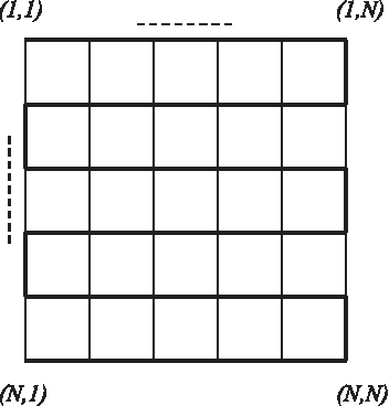
In any optimal solution to the above BLMP instance, \documentclass{aastex}\usepackage{amsbsy}\usepackage{amsfonts}\usepackage{amssymb}\usepackage{bm}\usepackage{mathrsfs}\usepackage{pifont}\usepackage{stmaryrd}\usepackage{textcomp}\usepackage{portland, xspace}\usepackage{amsmath, amsxtra}\pagestyle{empty}\DeclareMathSizes{10}{9}{7}{6}\begin{document}$$t_1 , t_2 , \ldots , t_{4N}$$\end{document} will lie on the boundary of the (N+1)×(N+1) grid (Fig. 1).

FIG. 1.
An illustration for Lemma 1 with N = 4. Each t_i lies on a dark vertex in the grid.

Proof

This can be proven by contradiction. Let T be the collection of the strings \documentclass{aastex}\usepackage{amsbsy}\usepackage{amsfonts}\usepackage{amssymb}\usepackage{bm}\usepackage{mathrsfs}\usepackage{pifont}\usepackage{stmaryrd}\usepackage{textcomp}\usepackage{portland, xspace}\usepackage{amsmath, amsxtra}\pagestyle{empty}\DeclareMathSizes{10}{9}{7}{6}\begin{document}$$t_1 , t_2 , \ldots , t_{4N}$$\end{document} . Let q be one of the strings from T that has a degree of 4 in an optimal placement. Let r be one of the strings equal to t that lies in the boundary. Next we show that we can get a better solution by exchanging q and r.

Let u be the number of neighbors of q from T. Let v be the number of neighbors of r from T. Note that 0 ≤ u ≤ 4 and 0 ≤ v ≤ 3. In the current solution, the total cost incurred by q and r is at least \documentclass{aastex}\usepackage{amsbsy}\usepackage{amsfonts}\usepackage{amssymb}\usepackage{bm}\usepackage{mathrsfs}\usepackage{pifont}\usepackage{stmaryrd}\usepackage{textcomp}\usepackage{portland, xspace}\usepackage{amsmath, amsxtra}\pagestyle{empty}\DeclareMathSizes{10}{9}{7}{6}\begin{document}$$\frac { 7 } { 4 } ku + k ( 4 - u ) + kv = \frac { 3 } { 4 } ku + kv + 4k$$\end{document} . If we exchange q and r, the new total cost incurred by q and r is strictly less than ku+2kv+k(3 − v)=ku+kv+3k. The old cost minus the new cost is strictly greater than \documentclass{aastex}\usepackage{amsbsy}\usepackage{amsfonts}\usepackage{amssymb}\usepackage{bm}\usepackage{mathrsfs}\usepackage{pifont}\usepackage{stmaryrd}\usepackage{textcomp}\usepackage{portland, xspace}\usepackage{amsmath, amsxtra}\pagestyle{empty}\DeclareMathSizes{10}{9}{7}{6}\begin{document}$$k - \frac { 1 } { 4 } ku \geq 0$$\end{document} .

We thus conclude that all the strings of T lie on the boundary of the grid in any optimal solution. ■

3.3. A special set of strings and some operations on strings

We denote the (ordered) concatenation of two strings x and y as x+y. If x and x′ (respectively y and y′) have the same length then, clearly, δ(x+y, x′+y′)=δ(x, x′)+δ(y, y′).

Given a string \documentclass{aastex}\usepackage{amsbsy}\usepackage{amsfonts}\usepackage{amssymb}\usepackage{bm}\usepackage{mathrsfs}\usepackage{pifont}\usepackage{stmaryrd}\usepackage{textcomp}\usepackage{portland, xspace}\usepackage{amsmath, amsxtra}\pagestyle{empty}\DeclareMathSizes{10}{9}{7}{6}\begin{document}$$x = \overline{x_1x_2 \ldots x_l}$$\end{document} and an integer h, let REP_h(x) be the string \documentclass{aastex}\usepackage{amsbsy}\usepackage{amsfonts}\usepackage{amssymb}\usepackage{bm}\usepackage{mathrsfs}\usepackage{pifont}\usepackage{stmaryrd}\usepackage{textcomp}\usepackage{portland, xspace}\usepackage{amsmath, amsxtra}\pagestyle{empty}\DeclareMathSizes{10}{9}{7}{6}\begin{document}$$\overline{x_1x_1 \ldots x_1 x_2x_2 \ldots x_2 \ldots x_lx_l \ldots x_l}$$\end{document} , where each x_i appears h times (REP stands for “replicate”). It is not hard to see that if x and y have the same length, then δ(REP_h(x), REP_h(y))=hδ(x, y).

Given an integer n, we can construct a set of n strings of length n each, \documentclass{aastex}\usepackage{amsbsy}\usepackage{amsfonts}\usepackage{amssymb}\usepackage{bm}\usepackage{mathrsfs}\usepackage{pifont}\usepackage{stmaryrd}\usepackage{textcomp}\usepackage{portland, xspace}\usepackage{amsmath, amsxtra}\pagestyle{empty}\DeclareMathSizes{10}{9}{7}{6}\begin{document}$$A_n = \{ a_1 , a_2 , \ldots , a_n \}$$\end{document} , such that δ(a_i, a_j)=2 for any 1 ≤ i ≠ j ≤ n. One way to construct A_n is to let \documentclass{aastex}\usepackage{amsbsy}\usepackage{amsfonts}\usepackage{amssymb}\usepackage{bm}\usepackage{mathrsfs}\usepackage{pifont}\usepackage{stmaryrd}\usepackage{textcomp}\usepackage{portland, xspace}\usepackage{amsmath, amsxtra}\pagestyle{empty}\DeclareMathSizes{10}{9}{7}{6}\begin{document}$$a_i = \overline{00 \ldots0100 \ldots0}$$\end{document} , where there are \documentclass{aastex}\usepackage{amsbsy}\usepackage{amsfonts}\usepackage{amssymb}\usepackage{bm}\usepackage{mathrsfs}\usepackage{pifont}\usepackage{stmaryrd}\usepackage{textcomp}\usepackage{portland, xspace}\usepackage{amsmath, amsxtra}\pagestyle{empty}\DeclareMathSizes{10}{9}{7}{6}\begin{document}$$( i - 1 ) \ \overline{0}$$\end{document} 's before \documentclass{aastex}\usepackage{amsbsy}\usepackage{amsfonts}\usepackage{amssymb}\usepackage{bm}\usepackage{mathrsfs}\usepackage{pifont}\usepackage{stmaryrd}\usepackage{textcomp}\usepackage{portland, xspace}\usepackage{amsmath, amsxtra}\pagestyle{empty}\DeclareMathSizes{10}{9}{7}{6}\begin{document}$$\overline{1}$$\end{document} . It is easy to check that δ(a_i, a_j)=2 for any 1 ≤ i ≠ j ≤ n.

3.4. Proof of the main theorem

Now we are ready to present the proof of Theorem 1. Let \documentclass{aastex}\usepackage{amsbsy}\usepackage{amsfonts}\usepackage{amssymb}\usepackage{bm}\usepackage{mathrsfs}\usepackage{pifont}\usepackage{stmaryrd}\usepackage{textcomp}\usepackage{portland, xspace}\usepackage{amsmath, amsxtra}\pagestyle{empty}\DeclareMathSizes{10}{9}{7}{6}\begin{document}$$S = \{ s_1 , s_2 , \ldots , s_{4N} \}$$\end{document} be the input for any instance of the 4N-strings HTSP. Each s_i has the length l. We will generate (N+1)² strings such that an optimal solution for the BLMP on these (N+1)² strings will yield an optimal solution for the 4N-strings HTSP on S.

The input for the BLMP instance that we generate will be \documentclass{aastex}\usepackage{amsbsy}\usepackage{amsfonts}\usepackage{amssymb}\usepackage{bm}\usepackage{mathrsfs}\usepackage{pifont}\usepackage{stmaryrd}\usepackage{textcomp}\usepackage{portland, xspace}\usepackage{amsmath, amsxtra}\pagestyle{empty}\DeclareMathSizes{10}{9}{7}{6}\begin{document}$$T = \{ t_1 , t_2 , \ldots , t_{4N} , t , t , \ldots , t \}$$\end{document} , where t occurs N² − 2N+1 times. We set t_i=REP_h(a_i)+REP₂(s_i), where a_i is the i-th string in the set A_4N defined in Section 3.3. We will choose h later. Also, we set \documentclass{aastex}\usepackage{amsbsy}\usepackage{amsfonts}\usepackage{amssymb}\usepackage{bm}\usepackage{mathrsfs}\usepackage{pifont}\usepackage{stmaryrd}\usepackage{textcomp}\usepackage{portland, xspace}\usepackage{amsmath, amsxtra}\pagestyle{empty}\DeclareMathSizes{10}{9}{7}{6}\begin{document}$$t = REP_{4Nh} ( \overline{0} ) + \overline{0101 \ldots01}$$\end{document} , where the string \documentclass{aastex}\usepackage{amsbsy}\usepackage{amsfonts}\usepackage{amssymb}\usepackage{bm}\usepackage{mathrsfs}\usepackage{pifont}\usepackage{stmaryrd}\usepackage{textcomp}\usepackage{portland, xspace}\usepackage{amsmath, amsxtra}\pagestyle{empty}\DeclareMathSizes{10}{9}{7}{6}\begin{document}$$\overline {01}$$\end{document} is repeated l times. We can easily check that: \documentclass{aastex}\usepackage{amsbsy}\usepackage{amsfonts}\usepackage{amssymb}\usepackage{bm}\usepackage{mathrsfs}\usepackage{pifont}\usepackage{stmaryrd}\usepackage{textcomp}\usepackage{portland, xspace}\usepackage{amsmath, amsxtra}\pagestyle{empty}\DeclareMathSizes{10}{9}{7}{6}\begin{document}\begin{align}\delta ( t_i , t ) = h + l \ \hbox{for any} \ 1 \leq i \leq 4N \tag{1}\end{align}\end{document} \documentclass{aastex}\usepackage{amsbsy}\usepackage{amsfonts}\usepackage{amssymb}\usepackage{bm}\usepackage{mathrsfs}\usepackage{pifont}\usepackage{stmaryrd}\usepackage{textcomp}\usepackage{portland, xspace}\usepackage{amsmath, amsxtra}\pagestyle{empty}\DeclareMathSizes{10}{9}{7}{6}\begin{document}\begin{align} \delta (t_i , t_j) = \, 2h + 2 \delta(s_i , s_j) \leq 2h + 2l \tag{2}\end{align}\end{document} \documentclass{aastex}\usepackage{amsbsy}\usepackage{amsfonts}\usepackage{amssymb}\usepackage{bm}\usepackage{mathrsfs}\usepackage{pifont}\usepackage{stmaryrd}\usepackage{textcomp}\usepackage{portland, xspace}\usepackage{amsmath, amsxtra}\pagestyle{empty}\DeclareMathSizes{10}{9}{7}{6}\begin{document}\begin{align}{\rm for \ any} \ 1 \leq i \neq j \leq 4N\end{align}\end{document}

We choose h so that T satisfies the condition in Lemma 1. Particularly, choose h=8l. Now we will show that OPT_BLMP(T)=4(N − 1)(h+l)+8Nh+2OPT_HTSP(S), which in turn means that an optimal solution for the BLMP on T will yield an optimal solution for the 4N-strings HTSP on S.

Let \documentclass{aastex}\usepackage{amsbsy}\usepackage{amsfonts}\usepackage{amssymb}\usepackage{bm}\usepackage{mathrsfs}\usepackage{pifont}\usepackage{stmaryrd}\usepackage{textcomp}\usepackage{portland, xspace}\usepackage{amsmath, amsxtra}\pagestyle{empty}\DeclareMathSizes{10}{9}{7}{6}\begin{document}$$A = s_{i_1} , s_{i_2} , \ldots , s_{i_{4N}}$$\end{document} be an optimal tour for the 4N-string HTSP on S. We construct a solution A′ for the BLMP on T by placing t_i's on the border of the grid in the order \documentclass{aastex}\usepackage{amsbsy}\usepackage{amsfonts}\usepackage{amssymb}\usepackage{bm}\usepackage{mathrsfs}\usepackage{pifont}\usepackage{stmaryrd}\usepackage{textcomp}\usepackage{portland, xspace}\usepackage{amsmath, amsxtra}\pagestyle{empty}\DeclareMathSizes{10}{9}{7}{6}\begin{document}$$t_{i_1} , t_{i_2} , \ldots , t_{i_{4N}}$$\end{document} and placing the copies of t on the center of the grid. By the equalities (1) and (2), the cost of A′ is Cost(A′)=4(N − 1)(h+l)+8Nh+2Cost(A). Therefore, OPT_BLMP(T) ≤ 4(N − 1)(h+l)+8Nh+2OPT_HTSP(S).

On the other hand, let B be an optimal solution for the BLMP on T. By Lemma 1, t_i's lie on the border of the grid, and the copies of t lie on the center of the grid. Assume that t_i's lie in the order \documentclass{aastex}\usepackage{amsbsy}\usepackage{amsfonts}\usepackage{amssymb}\usepackage{bm}\usepackage{mathrsfs}\usepackage{pifont}\usepackage{stmaryrd}\usepackage{textcomp}\usepackage{portland, xspace}\usepackage{amsmath, amsxtra}\pagestyle{empty}\DeclareMathSizes{10}{9}{7}{6}\begin{document}$$t_{i_1} , t_{i_2} , \ldots , t_{i_{4N}}$$\end{document} . We can construct a tour B′ for the 4N-strings HTSP on S in the order \documentclass{aastex}\usepackage{amsbsy}\usepackage{amsfonts}\usepackage{amssymb}\usepackage{bm}\usepackage{mathrsfs}\usepackage{pifont}\usepackage{stmaryrd}\usepackage{textcomp}\usepackage{portland, xspace}\usepackage{amsmath, amsxtra}\pagestyle{empty}\DeclareMathSizes{10}{9}{7}{6}\begin{document}$$s_{i_1} , s_{i_2} , \ldots , s_{i_{4N}}$$\end{document} . By the equalities (1) and (2), Cost(B)=4(N − 1)(h+l)+8Nh+2Cost(B′). Hence, OPT_BLMP(T) ≥ 4(N − 1)(h+l)+8Nh+2OPT_HTSP(S).

This completes the proof of Theorem 1. ■

3.5. \documentclass{aastex}\usepackage{amsbsy}\usepackage{amsfonts}\usepackage{amssymb}\usepackage{bm}\usepackage{mathrsfs}\usepackage{pifont}\usepackage{stmaryrd}\usepackage{textcomp}\usepackage{portland, xspace}\usepackage{amsmath, amsxtra}\pagestyle{empty}\DeclareMathSizes{10}{9}{7}{6}\begin{document}$${ \cal NP}$$\end{document} -hardness of the HGPMP for other special cases

We can generalize the result in Theorem 1 for other special cases of the HGPMP. We say graph G is “bordered-ring” if G is undirected and G has a ring of size Ω(n^α) for some constant α > 0 such that every vertex in the ring has degree no greater than d and every vertex outside the ring has degree greater than d for some d ≥ 3. For grid graphs, \documentclass{aastex}\usepackage{amsbsy}\usepackage{amsfonts}\usepackage{amssymb}\usepackage{bm}\usepackage{mathrsfs}\usepackage{pifont}\usepackage{stmaryrd}\usepackage{textcomp}\usepackage{portland, xspace}\usepackage{amsmath, amsxtra}\pagestyle{empty}\DeclareMathSizes{10}{9}{7}{6}\begin{document}$$\alpha = \frac { 1 } { 2 }$$\end{document} and d=3. Some variants of grid graphs like Manhattan grids are bordered-ring as well.

Theorem 3

The HGPMP is \documentclass{aastex}\usepackage{amsbsy}\usepackage{amsfonts}\usepackage{amssymb}\usepackage{bm}\usepackage{mathrsfs}\usepackage{pifont}\usepackage{stmaryrd}\usepackage{textcomp}\usepackage{portland, xspace}\usepackage{amsmath, amsxtra}\pagestyle{empty}\DeclareMathSizes{10}{9}{7}{6}\begin{document}$${ \cal NP}$$\end{document} -hard even if G is bordered-ring.

Proof

By a similar reduction to that of the BLMP above, the theorem follows. ■

3.6. An alternate \documentclass{aastex}\usepackage{amsbsy}\usepackage{amsfonts}\usepackage{amssymb}\usepackage{bm}\usepackage{mathrsfs}\usepackage{pifont}\usepackage{stmaryrd}\usepackage{textcomp}\usepackage{portland, xspace}\usepackage{amsmath, amsxtra}\pagestyle{empty}\DeclareMathSizes{10}{9}{7}{6}\begin{document}$${ \cal NP}$$\end{document} -hardness proof for the BLMP

In this section, we give an alternate \documentclass{aastex}\usepackage{amsbsy}\usepackage{amsfonts}\usepackage{amssymb}\usepackage{bm}\usepackage{mathrsfs}\usepackage{pifont}\usepackage{stmaryrd}\usepackage{textcomp}\usepackage{portland, xspace}\usepackage{amsmath, amsxtra}\pagestyle{empty}\DeclareMathSizes{10}{9}{7}{6}\begin{document}$${ \cal NP}$$\end{document} -hardness proof for the BLMP by showing that another variant of the HTSP, called k-segments HTSP, polynomially reduces to the BLMP. We believe that the techniques introduced in both of our proofs will find independent applications.

3.6.1. k-Segments traveling salesperson problem

We define the k-segments HTSP and show that it is NP-hard. Consider an input of n strings: \documentclass{aastex}\usepackage{amsbsy}\usepackage{amsfonts}\usepackage{amssymb}\usepackage{bm}\usepackage{mathrsfs}\usepackage{pifont}\usepackage{stmaryrd}\usepackage{textcomp}\usepackage{portland, xspace}\usepackage{amsmath, amsxtra}\pagestyle{empty}\DeclareMathSizes{10}{9}{7}{6}\begin{document}$$s_1 , s_2 , \ldots , s_n$$\end{document} . The problem of k-segments HTSP is to partition the n strings into k parts such that the sum of the optimal tour costs for the individual parts is minimum.

Theorem 4

The k-segments HTSP for strings is \documentclass{aastex}\usepackage{amsbsy}\usepackage{amsfonts}\usepackage{amssymb}\usepackage{bm}\usepackage{mathrsfs}\usepackage{pifont}\usepackage{stmaryrd}\usepackage{textcomp}\usepackage{portland, xspace}\usepackage{amsmath, amsxtra}\pagestyle{empty}\DeclareMathSizes{10}{9}{7}{6}\begin{document}$${ \cal NP}$$\end{document} -hard.

Proof

We will prove this for k=4 (since this is the instance that will be useful for us to prove the main result), and the theorem will then be obvious.

We will show that the HTSP polynomially reduces to the 4-segments HTSP. Let \documentclass{aastex}\usepackage{amsbsy}\usepackage{amsfonts}\usepackage{amssymb}\usepackage{bm}\usepackage{mathrsfs}\usepackage{pifont}\usepackage{stmaryrd}\usepackage{textcomp}\usepackage{portland, xspace}\usepackage{amsmath, amsxtra}\pagestyle{empty}\DeclareMathSizes{10}{9}{7}{6}\begin{document}$$S = \{ s_1 , s_2 , \ldots , s_n \}$$\end{document} be the input to any instance of the HTSP. We will generate an instance of the 4-segments HTSP that has as input (n+3) strings. Let l be the length of each string in S. Note that the optimal cost for the HTSP with input S is ≤nl.

Consider the 4 strings: \documentclass{aastex}\usepackage{amsbsy}\usepackage{amsfonts}\usepackage{amssymb}\usepackage{bm}\usepackage{mathrsfs}\usepackage{pifont}\usepackage{stmaryrd}\usepackage{textcomp}\usepackage{portland, xspace}\usepackage{amsmath, amsxtra}\pagestyle{empty}\DeclareMathSizes{10}{9}{7}{6}\begin{document}$$\overline {1110} , \overline {1101} , \overline {1011} , { \rm and} \ \overline {0111}$$\end{document} . The distance between any two of them is 2. Now replace each \documentclass{aastex}\usepackage{amsbsy}\usepackage{amsfonts}\usepackage{amssymb}\usepackage{bm}\usepackage{mathrsfs}\usepackage{pifont}\usepackage{stmaryrd}\usepackage{textcomp}\usepackage{portland, xspace}\usepackage{amsmath, amsxtra}\pagestyle{empty}\DeclareMathSizes{10}{9}{7}{6}\begin{document}$$\overline {1}$$\end{document} in each of these 4 strings with a string of nl \documentclass{aastex}\usepackage{amsbsy}\usepackage{amsfonts}\usepackage{amssymb}\usepackage{bm}\usepackage{mathrsfs}\usepackage{pifont}\usepackage{stmaryrd}\usepackage{textcomp}\usepackage{portland, xspace}\usepackage{amsmath, amsxtra}\pagestyle{empty}\DeclareMathSizes{10}{9}{7}{6}\begin{document}$$\overline {1}$$\end{document} 's. Also, replace each \documentclass{aastex}\usepackage{amsbsy}\usepackage{amsfonts}\usepackage{amssymb}\usepackage{bm}\usepackage{mathrsfs}\usepackage{pifont}\usepackage{stmaryrd}\usepackage{textcomp}\usepackage{portland, xspace}\usepackage{amsmath, amsxtra}\pagestyle{empty}\DeclareMathSizes{10}{9}{7}{6}\begin{document}$$\overline {0}$$\end{document} in each of these strings with a string of nl \documentclass{aastex}\usepackage{amsbsy}\usepackage{amsfonts}\usepackage{amssymb}\usepackage{bm}\usepackage{mathrsfs}\usepackage{pifont}\usepackage{stmaryrd}\usepackage{textcomp}\usepackage{portland, xspace}\usepackage{amsmath, amsxtra}\pagestyle{empty}\DeclareMathSizes{10}{9}{7}{6}\begin{document}$$\overline{0}$$\end{document} 's. Call these new strings t₁, t₂, t₃, t₄. The distance between any two of these strings is 2nl.

The input strings for the 4-segments HTSP are \documentclass{aastex}\usepackage{amsbsy}\usepackage{amsfonts}\usepackage{amssymb}\usepackage{bm}\usepackage{mathrsfs}\usepackage{pifont}\usepackage{stmaryrd}\usepackage{textcomp}\usepackage{portland, xspace}\usepackage{amsmath, amsxtra}\pagestyle{empty}\DeclareMathSizes{10}{9}{7}{6}\begin{document}$$q_1 , q_2 , \ldots , q_{n + 3}$$\end{document} and are constructed as follows: q_i is nothing but s_i with t₁ appended to the left, for 1 ≤ i ≤ n. Additionally, q_n₊₁ is a string of length 4nl+l whose l LSBs are \documentclass{aastex}\usepackage{amsbsy}\usepackage{amsfonts}\usepackage{amssymb}\usepackage{bm}\usepackage{mathrsfs}\usepackage{pifont}\usepackage{stmaryrd}\usepackage{textcomp}\usepackage{portland, xspace}\usepackage{amsmath, amsxtra}\pagestyle{empty}\DeclareMathSizes{10}{9}{7}{6}\begin{document}$$\overline{0}$$\end{document} 's and whose 4nl MSBs equal t₂; q_n₊₂ is a string of length 4nl+l whose l LSBs are \documentclass{aastex}\usepackage{amsbsy}\usepackage{amsfonts}\usepackage{amssymb}\usepackage{bm}\usepackage{mathrsfs}\usepackage{pifont}\usepackage{stmaryrd}\usepackage{textcomp}\usepackage{portland, xspace}\usepackage{amsmath, amsxtra}\pagestyle{empty}\DeclareMathSizes{10}{9}{7}{6}\begin{document}$$\overline{0}$$\end{document} and whose 4nl MSBs equal t₃. Also, q_n₊₃ has all \documentclass{aastex}\usepackage{amsbsy}\usepackage{amsfonts}\usepackage{amssymb}\usepackage{bm}\usepackage{mathrsfs}\usepackage{pifont}\usepackage{stmaryrd}\usepackage{textcomp}\usepackage{portland, xspace}\usepackage{amsmath, amsxtra}\pagestyle{empty}\DeclareMathSizes{10}{9}{7}{6}\begin{document}$$\overline{0}$$\end{document} 's in its l LSBs, and its 4nl MSBs equal t₄.

Clearly, in an optimal solution for the 4-segments HTSP instance, the four parts have to be \documentclass{aastex}\usepackage{amsbsy}\usepackage{amsfonts}\usepackage{amssymb}\usepackage{bm}\usepackage{mathrsfs}\usepackage{pifont}\usepackage{stmaryrd}\usepackage{textcomp}\usepackage{portland, xspace}\usepackage{amsmath, amsxtra}\pagestyle{empty}\DeclareMathSizes{10}{9}{7}{6}\begin{document}$$\{ q_1 , q_2 , \ldots , q_n \} , \ \{ q_{n + 1} \} , \ \{ q_{n + 2} \}$$\end{document} , and {q_n₊₃}. As a result, we can get an optimal solution for the HTSP instance given an optimal solution for the 4-segments HTSP instance. ■

3.6.2. A special instance of the BLMP

Consider the following n² strings as an input for the BLMP: \documentclass{aastex}\usepackage{amsbsy}\usepackage{amsfonts}\usepackage{amssymb}\usepackage{bm}\usepackage{mathrsfs}\usepackage{pifont}\usepackage{stmaryrd}\usepackage{textcomp}\usepackage{portland, xspace}\usepackage{amsmath, amsxtra}\pagestyle{empty}\DeclareMathSizes{10}{9}{7}{6}\begin{document}$$t_1 , t_2 , \ldots , t_{n} , t , t , \ldots , t$$\end{document} . Here there are n² − n copies of t. Also, δ(t_i, t_j)=16 for any i and j less than or equal to n, and δ(t_i, t)=9 for any i ≤ n.

Lemma 2

In an optimal solution to the above BLMP instance, \documentclass{aastex}\usepackage{amsbsy}\usepackage{amsfonts}\usepackage{amssymb}\usepackage{bm}\usepackage{mathrsfs}\usepackage{pifont}\usepackage{stmaryrd}\usepackage{textcomp}\usepackage{portland, xspace}\usepackage{amsmath, amsxtra}\pagestyle{empty}\DeclareMathSizes{10}{9}{7}{6}\begin{document}$$t_1 , t_2 , \ldots , t_n$$\end{document} lie on the boundary of the n×n grid and moreover these strings are found in four segments of successive nodes.

Proof

Let T be the collection of strings \documentclass{aastex}\usepackage{amsbsy}\usepackage{amsfonts}\usepackage{amssymb}\usepackage{bm}\usepackage{mathrsfs}\usepackage{pifont}\usepackage{stmaryrd}\usepackage{textcomp}\usepackage{portland, xspace}\usepackage{amsmath, amsxtra}\pagestyle{empty}\DeclareMathSizes{10}{9}{7}{6}\begin{document}$$t_1 , t_2 , \ldots , t_n$$\end{document} . By Lemma 1, we conclude that all the strings of T lie on the boundary of the grid in an optimal solution.

Let S₁ and S₂ be two segments such that S₁ and S₂ consist of strings from T, strings in S₁ are in successive nodes, strings in S₂ are in successive nodes, and these two segments are not successive. Consider the case in which none of these strings are in a corner of the grid. Let \documentclass{aastex}\usepackage{amsbsy}\usepackage{amsfonts}\usepackage{amssymb}\usepackage{bm}\usepackage{mathrsfs}\usepackage{pifont}\usepackage{stmaryrd}\usepackage{textcomp}\usepackage{portland, xspace}\usepackage{amsmath, amsxtra}\pagestyle{empty}\DeclareMathSizes{10}{9}{7}{6}\begin{document}$$S_1 = \{ a_1 , a_2 , \ldots , a_{n_1} \}$$\end{document} and \documentclass{aastex}\usepackage{amsbsy}\usepackage{amsfonts}\usepackage{amssymb}\usepackage{bm}\usepackage{mathrsfs}\usepackage{pifont}\usepackage{stmaryrd}\usepackage{textcomp}\usepackage{portland, xspace}\usepackage{amsmath, amsxtra}\pagestyle{empty}\DeclareMathSizes{10}{9}{7}{6}\begin{document}$$S_2 = \{ b_1 , b_2 , \ldots , b_{n_2} \}$$\end{document} . Let \documentclass{aastex}\usepackage{amsbsy}\usepackage{amsfonts}\usepackage{amssymb}\usepackage{bm}\usepackage{mathrsfs}\usepackage{pifont}\usepackage{stmaryrd}\usepackage{textcomp}\usepackage{portland, xspace}\usepackage{amsmath, amsxtra}\pagestyle{empty}\DeclareMathSizes{10}{9}{7}{6}\begin{document}$$C ( S_1 ) = \sum\nolimits_{i = 1}^{n_1 - 1} \delta ( a_i , a_{i + 1} )$$\end{document} and \documentclass{aastex}\usepackage{amsbsy}\usepackage{amsfonts}\usepackage{amssymb}\usepackage{bm}\usepackage{mathrsfs}\usepackage{pifont}\usepackage{stmaryrd}\usepackage{textcomp}\usepackage{portland, xspace}\usepackage{amsmath, amsxtra}\pagestyle{empty}\DeclareMathSizes{10}{9}{7}{6}\begin{document}$$C ( S_2 ) = \sum\nolimits_{i = 1}^{n_2 - 1} \delta ( b_i , b_{i + 1} )$$\end{document} . The total cost for these two segments is C(S₁)+C(S₂)+9(n₁+n₂)+36. If we join these two segments into one, the new cost will be C(S₁)+C(S₂)+9(n₁+n₂)+34.

Thus it follows that all the strings of T will be on the boundary, and they will be found in successive nodes in any optimal solution. Also it helps to utilize the corners of the grid since each use of a corner will reduce the total cost by nine. Therefore, in an optimal solution there will be four segments such that all the segments are in the boundary of the grid, each segment has strings from T in successive nodes, and one string of each segment occupies a corner of the grid. In other words, an optimal solution for the BLMP instance contains an optimal solution for the 4-segments TSP corresponding to T. The optimal cost for this BLMP instance is 25n − 28. ■

3.6.3. Construction of strings for the above BLMP instance

We can construct n² strings that have the same properties as the ones in the above BLMP instance. To begin with, we construct (n+1) binary strings of length n each. The string t_i has all \documentclass{aastex}\usepackage{amsbsy}\usepackage{amsfonts}\usepackage{amssymb}\usepackage{bm}\usepackage{mathrsfs}\usepackage{pifont}\usepackage{stmaryrd}\usepackage{textcomp}\usepackage{portland, xspace}\usepackage{amsmath, amsxtra}\pagestyle{empty}\DeclareMathSizes{10}{9}{7}{6}\begin{document}$$\overline{1}$$\end{document} 's except in position i, for 1 ≤ i ≤ n. The position of the LSB of any string is assumed to be \documentclass{aastex}\usepackage{amsbsy}\usepackage{amsfonts}\usepackage{amssymb}\usepackage{bm}\usepackage{mathrsfs}\usepackage{pifont}\usepackage{stmaryrd}\usepackage{textcomp}\usepackage{portland, xspace}\usepackage{amsmath, amsxtra}\pagestyle{empty}\DeclareMathSizes{10}{9}{7}{6}\begin{document}$$\overline{1}$$\end{document} . String t_n₊₁ has all \documentclass{aastex}\usepackage{amsbsy}\usepackage{amsfonts}\usepackage{amssymb}\usepackage{bm}\usepackage{mathrsfs}\usepackage{pifont}\usepackage{stmaryrd}\usepackage{textcomp}\usepackage{portland, xspace}\usepackage{amsmath, amsxtra}\pagestyle{empty}\DeclareMathSizes{10}{9}{7}{6}\begin{document}$$\overline{1}$$\end{document} 's. Clearly, δ(t_i, t_j)=2 for any i and j less than or equal to n. Also, δ(t_i, t_n₊₁)=1 for any 1 ≤ i ≤ n.

Now, in each t_i (for 1 ≤ i ≤ (n+1)), replace every \documentclass{aastex}\usepackage{amsbsy}\usepackage{amsfonts}\usepackage{amssymb}\usepackage{bm}\usepackage{mathrsfs}\usepackage{pifont}\usepackage{stmaryrd}\usepackage{textcomp}\usepackage{portland, xspace}\usepackage{amsmath, amsxtra}\pagestyle{empty}\DeclareMathSizes{10}{9}{7}{6}\begin{document}$$\overline{1}$$\end{document} with a string of eight \documentclass{aastex}\usepackage{amsbsy}\usepackage{amsfonts}\usepackage{amssymb}\usepackage{bm}\usepackage{mathrsfs}\usepackage{pifont}\usepackage{stmaryrd}\usepackage{textcomp}\usepackage{portland, xspace}\usepackage{amsmath, amsxtra}\pagestyle{empty}\DeclareMathSizes{10}{9}{7}{6}\begin{document}$$\overline{1}$$\end{document} 's and replace each \documentclass{aastex}\usepackage{amsbsy}\usepackage{amsfonts}\usepackage{amssymb}\usepackage{bm}\usepackage{mathrsfs}\usepackage{pifont}\usepackage{stmaryrd}\usepackage{textcomp}\usepackage{portland, xspace}\usepackage{amsmath, amsxtra}\pagestyle{empty}\DeclareMathSizes{10}{9}{7}{6}\begin{document}$$\overline{0}$$\end{document} with a string of eight \documentclass{aastex}\usepackage{amsbsy}\usepackage{amsfonts}\usepackage{amssymb}\usepackage{bm}\usepackage{mathrsfs}\usepackage{pifont}\usepackage{stmaryrd}\usepackage{textcomp}\usepackage{portland, xspace}\usepackage{amsmath, amsxtra}\pagestyle{empty}\DeclareMathSizes{10}{9}{7}{6}\begin{document}$$\overline{1}$$\end{document} 's. After this change, δ(t_i, t_j)=16 for any 1 ≤ i, j ≤ n and δ(t_i, t_n₊₁)=8 for any 1 ≤ i ≤ n.

Finally, append a \documentclass{aastex}\usepackage{amsbsy}\usepackage{amsfonts}\usepackage{amssymb}\usepackage{bm}\usepackage{mathrsfs}\usepackage{pifont}\usepackage{stmaryrd}\usepackage{textcomp}\usepackage{portland, xspace}\usepackage{amsmath, amsxtra}\pagestyle{empty}\DeclareMathSizes{10}{9}{7}{6}\begin{document}$$\overline{0}$$\end{document} to the left of each t_i (for 1 ≤ i ≤ n) as the MSB. Also, append a \documentclass{aastex}\usepackage{amsbsy}\usepackage{amsfonts}\usepackage{amssymb}\usepackage{bm}\usepackage{mathrsfs}\usepackage{pifont}\usepackage{stmaryrd}\usepackage{textcomp}\usepackage{portland, xspace}\usepackage{amsmath, amsxtra}\pagestyle{empty}\DeclareMathSizes{10}{9}{7}{6}\begin{document}$$\overline{1}$$\end{document} to the left of t_n₊₁. In this case, δ(t_i,t_j)=16 for any 1 ≤ i, j ≤ n and δ(t_i,t_n₊₁)=9 for any 1 ≤ i ≤ n.

3.6.4. The alternate proof of the main theorem

Let \documentclass{aastex}\usepackage{amsbsy}\usepackage{amsfonts}\usepackage{amssymb}\usepackage{bm}\usepackage{mathrsfs}\usepackage{pifont}\usepackage{stmaryrd}\usepackage{textcomp}\usepackage{portland, xspace}\usepackage{amsmath, amsxtra}\pagestyle{empty}\DeclareMathSizes{10}{9}{7}{6}\begin{document}$$S = \{ s_1 , s_2 , \ldots , s_n \}$$\end{document} be the input for any instance of the HTSP. We will generate n² strings such that an optimal solution for the BLMP on these n² strings will yield an optimal solution for the 4-segments HTSP on S.

We will use as the basis the (n+1) strings generated in the above section. Recall that these strings \documentclass{aastex}\usepackage{amsbsy}\usepackage{amsfonts}\usepackage{amssymb}\usepackage{bm}\usepackage{mathrsfs}\usepackage{pifont}\usepackage{stmaryrd}\usepackage{textcomp}\usepackage{portland, xspace}\usepackage{amsmath, amsxtra}\pagestyle{empty}\DeclareMathSizes{10}{9}{7}{6}\begin{document}$$t_1 , t_2 , \ldots , t_{n + 1}$$\end{document} are of length (8n+1) each. Also, δ(t_i, t_j)=16 for any 1 ≤ i, j ≤ n and δ(t_i, t_n₊₁)=9 for any 1 ≤ i ≤ n.

Replace each \documentclass{aastex}\usepackage{amsbsy}\usepackage{amsfonts}\usepackage{amssymb}\usepackage{bm}\usepackage{mathrsfs}\usepackage{pifont}\usepackage{stmaryrd}\usepackage{textcomp}\usepackage{portland, xspace}\usepackage{amsmath, amsxtra}\pagestyle{empty}\DeclareMathSizes{10}{9}{7}{6}\begin{document}$$\overline{0}$$\end{document} in each of the above strings with nl \documentclass{aastex}\usepackage{amsbsy}\usepackage{amsfonts}\usepackage{amssymb}\usepackage{bm}\usepackage{mathrsfs}\usepackage{pifont}\usepackage{stmaryrd}\usepackage{textcomp}\usepackage{portland, xspace}\usepackage{amsmath, amsxtra}\pagestyle{empty}\DeclareMathSizes{10}{9}{7}{6}\begin{document}$$\overline{0}$$\end{document} 's and replace each \documentclass{aastex}\usepackage{amsbsy}\usepackage{amsfonts}\usepackage{amssymb}\usepackage{bm}\usepackage{mathrsfs}\usepackage{pifont}\usepackage{stmaryrd}\usepackage{textcomp}\usepackage{portland, xspace}\usepackage{amsmath, amsxtra}\pagestyle{empty}\DeclareMathSizes{10}{9}{7}{6}\begin{document}$$\overline{1}$$\end{document} in each of these strings with nl \documentclass{aastex}\usepackage{amsbsy}\usepackage{amsfonts}\usepackage{amssymb}\usepackage{bm}\usepackage{mathrsfs}\usepackage{pifont}\usepackage{stmaryrd}\usepackage{textcomp}\usepackage{portland, xspace}\usepackage{amsmath, amsxtra}\pagestyle{empty}\DeclareMathSizes{10}{9}{7}{6}\begin{document}$$\overline{1}$$\end{document} 's. Now, δ(t_i,t_j)=16nl for any 1 ≤ i, j ≤ n, and δ(t_i,t_n₊₁)=9nl for any 1 ≤ i ≤ n. Each of these strings is of length (8n+1)nl.

Replace each \documentclass{aastex}\usepackage{amsbsy}\usepackage{amsfonts}\usepackage{amssymb}\usepackage{bm}\usepackage{mathrsfs}\usepackage{pifont}\usepackage{stmaryrd}\usepackage{textcomp}\usepackage{portland, xspace}\usepackage{amsmath, amsxtra}\pagestyle{empty}\DeclareMathSizes{10}{9}{7}{6}\begin{document}$$\overline{0}$$\end{document} in each s_i with two \documentclass{aastex}\usepackage{amsbsy}\usepackage{amsfonts}\usepackage{amssymb}\usepackage{bm}\usepackage{mathrsfs}\usepackage{pifont}\usepackage{stmaryrd}\usepackage{textcomp}\usepackage{portland, xspace}\usepackage{amsmath, amsxtra}\pagestyle{empty}\DeclareMathSizes{10}{9}{7}{6}\begin{document}$$\overline{0}$$\end{document} 's (for 1 ≤ i ≤ n), and replace each \documentclass{aastex}\usepackage{amsbsy}\usepackage{amsfonts}\usepackage{amssymb}\usepackage{bm}\usepackage{mathrsfs}\usepackage{pifont}\usepackage{stmaryrd}\usepackage{textcomp}\usepackage{portland, xspace}\usepackage{amsmath, amsxtra}\pagestyle{empty}\DeclareMathSizes{10}{9}{7}{6}\begin{document}$$\overline{1}$$\end{document} in each s_i with two \documentclass{aastex}\usepackage{amsbsy}\usepackage{amsfonts}\usepackage{amssymb}\usepackage{bm}\usepackage{mathrsfs}\usepackage{pifont}\usepackage{stmaryrd}\usepackage{textcomp}\usepackage{portland, xspace}\usepackage{amsmath, amsxtra}\pagestyle{empty}\DeclareMathSizes{10}{9}{7}{6}\begin{document}$$\overline{1}$$\end{document} 's and let s_i′ be the resultant string. Note that an optimal solution for the 4-segments HTSP on the revised S will also be an optimal solution for the 4-segments HTSP on the old S. If l is the length of each string in the old S, then 2l will be the length of each revised input string.

The input for the BLMP instance that we generate will be \documentclass{aastex}\usepackage{amsbsy}\usepackage{amsfonts}\usepackage{amssymb}\usepackage{bm}\usepackage{mathrsfs}\usepackage{pifont}\usepackage{stmaryrd}\usepackage{textcomp}\usepackage{portland, xspace}\usepackage{amsmath, amsxtra}\pagestyle{empty}\DeclareMathSizes{10}{9}{7}{6}\begin{document}$$q_1 , q_2 , \ldots , q_n , t , t , \ldots , t$$\end{document} , where t occurs n² − n times. Each of these strings will be of length (8n+1)nl+2l. The string q_i will have s_i′ in its 2l LSBs, and it will have t_i in its (8n+1)nl MSBs, for 1 ≤ i ≤ n. The string t will have t_n₊₁ in its (8n+1)nl MSBs. Its 2l LSBs will be \documentclass{aastex}\usepackage{amsbsy}\usepackage{amsfonts}\usepackage{amssymb}\usepackage{bm}\usepackage{mathrsfs}\usepackage{pifont}\usepackage{stmaryrd}\usepackage{textcomp}\usepackage{portland, xspace}\usepackage{amsmath, amsxtra}\pagestyle{empty}\DeclareMathSizes{10}{9}{7}{6}\begin{document}$$\overline{0101 \ldots 01}$$\end{document} , that is, the string \documentclass{aastex}\usepackage{amsbsy}\usepackage{amsfonts}\usepackage{amssymb}\usepackage{bm}\usepackage{mathrsfs}\usepackage{pifont}\usepackage{stmaryrd}\usepackage{textcomp}\usepackage{portland, xspace}\usepackage{amsmath, amsxtra}\pagestyle{empty}\DeclareMathSizes{10}{9}{7}{6}\begin{document}$$\overline {01}$$\end{document} is repeated l times. Note that δ(q_i, q_j)=16nl+δ(s_i′, s_j′) for any 1 ≤ i, j ≤ n. Also, δ(q_i, t)=9nl+l for any 1 ≤ i ≤ n.

Note that strings of this BLMP instance are comparable to the strings we had for Lemma 2. This is because the interstring distances are very nearly in the same ratios for the two cases. As a result, using a proof similar to that of Lemma 2, we can show that the strings \documentclass{aastex}\usepackage{amsbsy}\usepackage{amsfonts}\usepackage{amssymb}\usepackage{bm}\usepackage{mathrsfs}\usepackage{pifont}\usepackage{stmaryrd}\usepackage{textcomp}\usepackage{portland, xspace}\usepackage{amsmath, amsxtra}\pagestyle{empty}\DeclareMathSizes{10}{9}{7}{6}\begin{document}$$t_1 , t_2 , \ldots , t_n$$\end{document} will all lie in the boundary of the grid in an optimal solution to the above BLMP. Let \documentclass{aastex}\usepackage{amsbsy}\usepackage{amsfonts}\usepackage{amssymb}\usepackage{bm}\usepackage{mathrsfs}\usepackage{pifont}\usepackage{stmaryrd}\usepackage{textcomp}\usepackage{portland, xspace}\usepackage{amsmath, amsxtra}\pagestyle{empty}\DeclareMathSizes{10}{9}{7}{6}\begin{document}$$T = \{ t_1 , t_2 , \ldots , t_n \}$$\end{document} . Also, the strings of T will be found in four segments such that one string of each segment occupies one of the corner nodes of the grid. Let S₁, S₂, S₃, and S₄ stand for the strings in these four segments, respectively. Let C₁, C₂, C₃, and C₄ be the optimal tour costs for S₁, S₂, S₃, and S₄, respectively.

Let |S_i|=n_i for 1 ≤ i ≤ 4. The total cost (i.e., the border length) for the above BLMP solution can be computed as follows. Consider S₁ alone. The cost because of this segment is C₁+2(9nl+l)+(n₁ − 1)(9nl+l). The cost 2(9nl+l) is due to the two end points of the segment S₁. The cost (n₁ − 1)(9nl+l) is because each string of S₁ (except for the one in a corner of the grid) is a neighbor of a t. Upon simplification, the cost for S₁ is C₁+(n₁+1)(9nl+l). Summing over all the four segments, the total cost for the BLMP solution is C₁+C₂+C₃+C₄+(n+4)(9nl+l). The minimum value of this is obtained when S₁, S₂, S₃, and S₄ form a solution to the 4-segments HTSP on T.

Clearly, an optimal solution for the 4-segments HTSP on T will also yield an optimal solution for the 4-segments HTSP on S. This can be seen as follows. Consider the strings in S_i and let \documentclass{aastex}\usepackage{amsbsy}\usepackage{amsfonts}\usepackage{amssymb}\usepackage{bm}\usepackage{mathrsfs}\usepackage{pifont}\usepackage{stmaryrd}\usepackage{textcomp}\usepackage{portland, xspace}\usepackage{amsmath, amsxtra}\pagestyle{empty}\DeclareMathSizes{10}{9}{7}{6}\begin{document}$$Q_i = a^i_1 , a^i_2 , \ldots , a^i_{n_i}$$\end{document} be the corresponding input strings (of S), for 1 ≤ i ≤ 4. Note that C_i is nothing but (n_i − 1)(16nl) plus twice the optimal tour cost for Q_i, for 1 ≤ i ≤ 4. Thus, C₁+C₂+C₃+C₄ is equal to (n − 4)16nl+2(C₁′+C₂′+C₃′+C₄′) where C_i′ is the optimal tour cost for Q_i, for 1 ≤ i ≤ 4.

This completes the proof of Theorem 1. ■

4. Algorithms For The Blmp

4.1. An O(N)-approximation algorithm

In this section, we will show that a simple version of the algorithm suggested by Hannenhalli et al. (2002) is actually an O(N)-approximation algorithm. This algorithm can be described as follows. Assume that the input is the set of strings \documentclass{aastex}\usepackage{amsbsy}\usepackage{amsfonts}\usepackage{amssymb}\usepackage{bm}\usepackage{mathrsfs}\usepackage{pifont}\usepackage{stmaryrd}\usepackage{textcomp}\usepackage{portland, xspace}\usepackage{amsmath, amsxtra}\pagestyle{empty}\DeclareMathSizes{10}{9}{7}{6}\begin{document}$$S = \{ s_1 , s_2 , \ldots , s_{N^2} \}$$\end{document} . The algorithm first computes a tour T on strings in S. Then it threads the tour T into the grid in row-major order (Fig. 2). The first step can be done by calling the \documentclass{aastex}\usepackage{amsbsy}\usepackage{amsfonts}\usepackage{amssymb}\usepackage{bm}\usepackage{mathrsfs}\usepackage{pifont}\usepackage{stmaryrd}\usepackage{textcomp}\usepackage{portland, xspace}\usepackage{amsmath, amsxtra}\pagestyle{empty}\DeclareMathSizes{10}{9}{7}{6}\begin{document}$$\frac {3} {2}$$\end{document} -approximation algorithm for the HTSP as suggested by Christofides (1976).

FIG. 2.
The thick dark line corresponds to an optimal tour on the input strings.

Lemma 3

OPT_HTSP(S) ≤ 2OPT_BLMP(S).

Proof

Let A be an optimal solution for the BLMP on S. Consider the path P′ drawn as the thick dark line in Figure 2. Obviously, Cost(P′) ≤ Cost(A)=OPT_BLMP(S). Let \documentclass{aastex}\usepackage{amsbsy}\usepackage{amsfonts}\usepackage{amssymb}\usepackage{bm}\usepackage{mathrsfs}\usepackage{pifont}\usepackage{stmaryrd}\usepackage{textcomp}\usepackage{portland, xspace}\usepackage{amsmath, amsxtra}\pagestyle{empty}\DeclareMathSizes{10}{9}{7}{6}\begin{document}$$s_{i_1}$$\end{document} and \documentclass{aastex}\usepackage{amsbsy}\usepackage{amsfonts}\usepackage{amssymb}\usepackage{bm}\usepackage{mathrsfs}\usepackage{pifont}\usepackage{stmaryrd}\usepackage{textcomp}\usepackage{portland, xspace}\usepackage{amsmath, amsxtra}\pagestyle{empty}\DeclareMathSizes{10}{9}{7}{6}\begin{document}$$s_{i_{N^2}}$$\end{document} be the two endpoints of P′. Since the Hamming distance satisfies the triangular inequality, \documentclass{aastex}\usepackage{amsbsy}\usepackage{amsfonts}\usepackage{amssymb}\usepackage{bm}\usepackage{mathrsfs}\usepackage{pifont}\usepackage{stmaryrd}\usepackage{textcomp}\usepackage{portland, xspace}\usepackage{amsmath, amsxtra}\pagestyle{empty}\DeclareMathSizes{10}{9}{7}{6}\begin{document}$$\delta ( s_{i_1} , s_{i_{N^2}} ) \leq Cost ( P^{ \prime}$$\end{document} ). Consider the tour that starts at \documentclass{aastex}\usepackage{amsbsy}\usepackage{amsfonts}\usepackage{amssymb}\usepackage{bm}\usepackage{mathrsfs}\usepackage{pifont}\usepackage{stmaryrd}\usepackage{textcomp}\usepackage{portland, xspace}\usepackage{amsmath, amsxtra}\pagestyle{empty}\DeclareMathSizes{10}{9}{7}{6}\begin{document}$$s_{i_1}$$\end{document} , traverses along the path P′ to \documentclass{aastex}\usepackage{amsbsy}\usepackage{amsfonts}\usepackage{amssymb}\usepackage{bm}\usepackage{mathrsfs}\usepackage{pifont}\usepackage{stmaryrd}\usepackage{textcomp}\usepackage{portland, xspace}\usepackage{amsmath, amsxtra}\pagestyle{empty}\DeclareMathSizes{10}{9}{7}{6}\begin{document}$$s_{i_{N^2}}$$\end{document} , and comes back to \documentclass{aastex}\usepackage{amsbsy}\usepackage{amsfonts}\usepackage{amssymb}\usepackage{bm}\usepackage{mathrsfs}\usepackage{pifont}\usepackage{stmaryrd}\usepackage{textcomp}\usepackage{portland, xspace}\usepackage{amsmath, amsxtra}\pagestyle{empty}\DeclareMathSizes{10}{9}{7}{6}\begin{document}$$s_{i_1}$$\end{document} . Obviously, the cost of the tour is \documentclass{aastex}\usepackage{amsbsy}\usepackage{amsfonts}\usepackage{amssymb}\usepackage{bm}\usepackage{mathrsfs}\usepackage{pifont}\usepackage{stmaryrd}\usepackage{textcomp}\usepackage{portland, xspace}\usepackage{amsmath, amsxtra}\pagestyle{empty}\DeclareMathSizes{10}{9}{7}{6}\begin{document}$$Cost ( P^{ \prime} ) + \delta ( s_{i_1} , s_{i_{N^2}} ) \leq 2Cost ( P^{ \prime} ) \leq 2Cost ( A )$$\end{document} . Hence, OPT_HTSP(S) ≤ 2OPT_BLMP(S). ■

Theorem 5

The above algorithm yields an O(N)-approximate solution.

Proof

First, we see that \documentclass{aastex}\usepackage{amsbsy}\usepackage{amsfonts}\usepackage{amssymb}\usepackage{bm}\usepackage{mathrsfs}\usepackage{pifont}\usepackage{stmaryrd}\usepackage{textcomp}\usepackage{portland, xspace}\usepackage{amsmath, amsxtra}\pagestyle{empty}\DeclareMathSizes{10}{9}{7}{6}\begin{document}$$Cost ( T ) \leq \frac { 3 } { 2 } OPT_ { HTSP } ( S ) \leq 3OPT_ { BLMP } ( S )$$\end{document} . The first inequality is due to the \documentclass{aastex}\usepackage{amsbsy}\usepackage{amsfonts}\usepackage{amssymb}\usepackage{bm}\usepackage{mathrsfs}\usepackage{pifont}\usepackage{stmaryrd}\usepackage{textcomp}\usepackage{portland, xspace}\usepackage{amsmath, amsxtra}\pagestyle{empty}\DeclareMathSizes{10}{9}{7}{6}\begin{document}$$\frac { 3 } { 2 }$$\end{document} -approximation for the HTSP. The second inequality is due to Lemma 3. Now let us analyze the cost of the solution F produced by the algorithm. Consider the path P drawn as the thick dark line in Figure 2. Obviously, Cost(P) ≤ Cost(T). Also, the total cost of the N rows in F is no more than Cost(P). By the triangle inequality, it is not hard to see that the cost of each column in F is no more than Cost(P). Therefore, Cost(F) ≤ (N+1)Cost(P) ≤ (N+1)Cost(T) ≤ 3(N+1)OPT_BLMP(S)=O(N)OPT_BLMP(S). ■

4.2. A hierarchical refinement algorithm

Several heuristics such as the epitaxial growth have been proposed to solve the BLMP problem earlier. However, most of these heuristics do not improve the cost monotonically. Local search-based algorithms are often employed to solve hard combinatorial problems. We now introduce a hierarchical refinement algorithm (HRA). This refinement technique can be applied to any heuristic placement to refine the cost and obtain a better placement. Let N be the number of probes in the placement, d a positive integer such that d^x=N, and x ≥ 1 is called the degree of refinement. The refinement algorithm starts with a given placement, then it divides the placement into \documentclass{aastex}\usepackage{amsbsy}\usepackage{amsfonts}\usepackage{amssymb}\usepackage{bm}\usepackage{mathrsfs}\usepackage{pifont}\usepackage{stmaryrd}\usepackage{textcomp}\usepackage{portland, xspace}\usepackage{amsmath, amsxtra}\pagestyle{empty}\DeclareMathSizes{10}{9}{7}{6}\begin{document}$$s^0_1 , s^0_2 \ldots s^0_{N / d^2}$$\end{document} subproblems with d² probes per subproblem. Each of these subproblems is solved optimally—an optimal permutation among the probes is found. After this every d² subproblems are combined into a new subproblem \documentclass{aastex}\usepackage{amsbsy}\usepackage{amsfonts}\usepackage{amssymb}\usepackage{bm}\usepackage{mathrsfs}\usepackage{pifont}\usepackage{stmaryrd}\usepackage{textcomp}\usepackage{portland, xspace}\usepackage{amsmath, amsxtra}\pagestyle{empty}\DeclareMathSizes{10}{9}{7}{6}\begin{document}$$s^1_i = \displaystyle \cup_{j = 1}^{d^2} s^0_{id^2 + j} , 1 \leq i \leq N / d^3$$\end{document} . To solve \documentclass{aastex}\usepackage{amsbsy}\usepackage{amsfonts}\usepackage{amssymb}\usepackage{bm}\usepackage{mathrsfs}\usepackage{pifont}\usepackage{stmaryrd}\usepackage{textcomp}\usepackage{portland, xspace}\usepackage{amsmath, amsxtra}\pagestyle{empty}\DeclareMathSizes{10}{9}{7}{6}\begin{document}$$s^1_i$$\end{document} optimally, we identify an optimal permutation among \documentclass{aastex}\usepackage{amsbsy}\usepackage{amsfonts}\usepackage{amssymb}\usepackage{bm}\usepackage{mathrsfs}\usepackage{pifont}\usepackage{stmaryrd}\usepackage{textcomp}\usepackage{portland, xspace}\usepackage{amsmath, amsxtra}\pagestyle{empty}\DeclareMathSizes{10}{9}{7}{6}\begin{document}$$s^0_{id^2 + j} \in s^1_i , 1 \leq j \leq d^2$$\end{document} . This process continues until we are left with no subproblems to solve (Fig. 3).

FIG. 3.
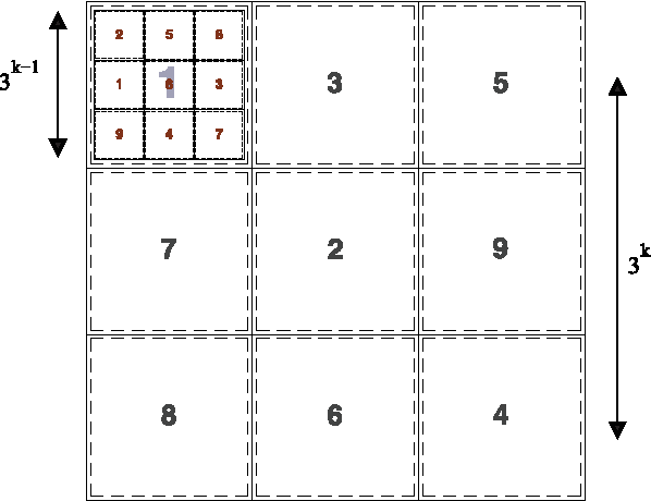
Illustration of the hierarchical refinement algorithm with degree of refinement 3. This shows the possible optimal solutions (i.e., permutation among subproblems) at the top-most and penultimate levels.

We should remark that while solving a subproblem optimally, we also consider the cost contributed from the neighboring subproblems. This ensures the monotonic improvement in the placement cost. The refinement algorithm asymptotically runs in Θ(d²!N) time. If d=O(1), the refinement algorithm runs in linear time. For small values of d, the algorithm performs well in practice. HRA is a deterministic refinement algorithm. We further extend this by introducing randomness. The randomized hierarchical refinement algorithm (RHRA) is similar to the HRA algorithm. RHRA randomly selects a subsquare within the given placement and applies the HRA technique to the selected subsquare. Similar to local search algorithms, repeating RHRA algorithm several times improves the placement cost monotonically. We study the performance of both these algorithms in Section 5.

4.3. Quad epitaxial algorithm

The epitaxial (EPX) placement suggested in Kahng et al. (2003) places a randomly selected probe at the center of the array, it continues placing the probes greedily around the locations adjacent to the placed probes to minimize the cost (i.e., the algorithm almost spends O(N²) time to place each probe). The epitaxial algorithm gives good results for small arrays, but for larger arrays the epitaxial algorithm is impractical and extremely slow. We propose the quad epitaxial (QEPX) algorithm as a simple extension to the epitaxial algorithm. QEPX yields good performance and is very fast compared to the EPX algorithm. The basic idea behind the QEPX algorithm is to divide the array into four parts, apply EPX algorithm for each of the four parts, and finally find an optimal arrangement among the four parts. In Section 5, we compare the QEPX algorithm with EPX algorithm.

5. Experimental Study

5.1. Performance of the QEPX algorithm

In this section, we compare the performance of QEPX algorithm introduced earlier. We use randomly generated probe arrays of size 32², 64², 128², and 256². In all of our experimental studies we compute a lower bound on the solution by picking the smallest 2N(N − 1) edges from the complete Hamming distance graph. Column 4 (Init Cost) in Table 1 indicates the placement cost obtained by placing the probes in the row-major order as given by the input. Column 5 indicates the final placement cost obtained by the epitaxial (quad) algorithm. As we can see from columns 7 and 10, the refinement obtained by the QEPX algorithm is very close to the EPX algorithm. On the other hand, QEPX runs 3.6×faster than the EPX algorithm. As we can see from Table1, as the chip size increases, EPX algorithm becomes very slow. We ran both EPX and QEPX algorithms on a chip size of 243×243 with a time limit of 60 minutes. The QEPX algorithm took around 12 minutes to complete and improved the input placement cost by 36%. On the other hand, the EPX algorithm did not complete the placement. From our experiments we conclude that the QEPX can provide a good placement, which we can use as an input for refinement/local search algorithms such as RHRA. In the next subsection we provide our experimental study of HRA and RHRA algorithms on various placement heuristics.

Table 1.
Comparison Between Epitaxial and Quad Epitaxial

Test Case Probes Lower Bound Init Cost EPX Time (sec) Refined Percent QEPX Time (sec) Refined Percent

t-0 1024 23480 37192 27591 0.60 25.81% 28060 0.42 24.55%

t-1 1024 23427 37029 27472 0.62 25.81% 28151 0.43 23.98%

t-0 4096 86818 151116 106471 10.70 29.54% 107805 3.05 28.66%

t-1 4096 86897 151176 106430 10.37 29.60% 107634 3.23 28.80%

t-0 16384 322129 609085 410301 180.00 32.64% 411746 43.93 32.40%

t-1 16384 — 608928 409625 185.88 32.73% 410902 44.70 32.52%

t-0 65536 — 2447885 2447885 — 0.00% 1563369 765.79 36.13%

t-1 65536 — 2427143 2427143 — 0.00% 1562630 774.33 35.62%

5.2. Performance of refinement algorithms

We have applied our HRA and RHRA refining algorithms on the following placement heuristics.

— (RAND) Random placement: In this placement, we use the order in which the probes are provided to our algorithm.

— (SORT) Sort placement: In this placement, the input probes are sorted lexicographically.

— (SWM) Sliding window matching placement is obtained by running the SWM (Kahng et al., 2003) algorithm with parameters (6, 3).

— (REPX) Row epitaxial placement is obtained by running the row-epitaxial algorithm with three look-ahead rows.

— (EPX) Epitaxial placement is obtained by running the EPX algorithm.

— (QEPX) Quad epitaxial placement is obtained by our quad-epitaxial algorithm.

The cost of the placement obtained by running the HRA algorithm exactly once is given in column 5 (HRA). Column 6 (RHRA) indicates the placement cost obtained by running our randomized refinement algorithm RHRA for 350 iterations. From Table 2 we can see that as initial placement moves closer and closer toward the lower bound, the refinement percentage decreases, which is logical. For test cases with 729, 6561 (1024, 4096) probes we use a refinement degree d=3 (d=2). Choosing a bigger refinement degree gives better refinements, however, takes more time. Finally we conclude that our refinement algorithms would be very useful when applied in conjunction with fast initial placement heuristics.

Table 2.
Cost Refinement for Various Placement Heuristics by Applying HRA (Hierarchical Refinement Algorithm) and RHRA (Randomized Hierarchical Refinement Algorithm) with 350 Iterations

Probes Algo Lower Bound Init Cost HRA RHRA Refined Percent Time

729 RAND 17087 26401 23970 22631 14.280% 2.83 (min)

729 SORT 17087 24082 22415 21649 10.103% 2.81 (min)

729 SWM 17087 22267 22195 22069 0.889% 2.81 (min)

729 REPTX 17087 21115 21107 21101 0.066% 2.81 (min)

729 EPTX 17087 19733 19726 19726 0.035% 2.81 (min)

6561 RAND 136820 243125 221090 209514 13.825% 17.55 (min)

6561 SORT 136820 210326 198972 191915 8.754% 17.02 (min)

6561 SWM 136820 204955 204525 203412 0.753% 17.20 (min)

6561 REPTX 136820 185386 185362 185341 0.024% 17.16 (min)

6561 EPTX 136820 168676 168623 168544 0.078% 17.15 (min)

1024 RAND 23480 37192 35236 33046 11.148% 0.28 (sec)

1024 SORT 23480 33784 32326 31026 8.164% 0.26 (sec)

1024 SWM 23480 31424 31383 31323 0.321% 0.13 (sec)

1024 QEPX 23480 28060 28035 28028 0.114% 0.47 (sec)

1024 REPTX 23480 29574 29557 29546 0.095% 0.11 (sec)

1024 EPTX 23480 27591 27567 27565 0.094% 0.11 (sec)

4096 RAND 86818 151116 143246 134485 11.005% 6.93 (sec)

4096 SORT 86818 131291 127033 121742 7.273% 4.46 (sec)

4096 SWM 86818 127516 127357 127092 0.333% 1.27 (sec)

4096 QEPX 86818 107805 107766 107702 0.096% 5.04 (sec)

4096 REPTX 86818 116406 116395 116376 0.026% 1.02 (sec)

4096 EPTX 86818 106471 106462 106448 0.022% 1.04 (sec)

6. Conclusions

In this article, we have studied the border length minimization problem (BLMP), which has numerous applications in biology and medicine. We solved a seven-year-old open problem in this area by showing that the BLMP is \documentclass{aastex}\usepackage{amsbsy}\usepackage{amsfonts}\usepackage{amssymb}\usepackage{bm}\usepackage{mathrsfs}\usepackage{pifont}\usepackage{stmaryrd}\usepackage{textcomp}\usepackage{portland, xspace}\usepackage{amsmath, amsxtra}\pagestyle{empty}\DeclareMathSizes{10}{9}{7}{6}\begin{document}$${ \cal NP}$$\end{document} -hard. Two different proofs have been given, and we believe that the techniques in these proofs will find independent applications. We have also shown that certain generalizations of the BLMP are \documentclass{aastex}\usepackage{amsbsy}\usepackage{amsfonts}\usepackage{amssymb}\usepackage{bm}\usepackage{mathrsfs}\usepackage{pifont}\usepackage{stmaryrd}\usepackage{textcomp}\usepackage{portland, xspace}\usepackage{amsmath, amsxtra}\pagestyle{empty}\DeclareMathSizes{10}{9}{7}{6}\begin{document}$${ \cal NP}$$\end{document} -hard as well. In addition, we have presented a hierarchical refinement algorithm (HRA) for the BLMP. Deterministic and randomized versions of this algorithm can be used to refine the solutions obtained from any algorithm for solving the BLMP. Our experimental results indicate that indeed HRA can be useful in practice.

One of the best-performing algorithms for the BLMP is the epitaxial algorithm (EPX). This algorithm takes too much time, especially when the number of probes is large. In this article we present a variant called the quad-epitaxial algorithm (QEPX), which is much faster than EPX while yielding a solution that is very close to that of EPX in quality. QEPX partitions the input into four parts, works on each part separately, and finally combines these solutions. This idea can be extended further to partition the input into more parts and hence this algorithm is ideal for parallelism.

Some of the additional goals are: 1) We have used a simple lower bound on the quality of solution for the BLMP, and it would be nice to develop tighter lower bounds; 2) to develop more efficient algorithms than EPX; and 3) to design parallel algorithms for the BLMP.

Test Case	Probes	Lower Bound	Init Cost	EPX	Time (sec)	Refined Percent	QEPX	Time (sec)	Refined Percent
t-0	1024	23480	37192	27591	0.60	25.81%	28060	0.42	24.55%
t-1	1024	23427	37029	27472	0.62	25.81%	28151	0.43	23.98%
t-0	4096	86818	151116	106471	10.70	29.54%	107805	3.05	28.66%
t-1	4096	86897	151176	106430	10.37	29.60%	107634	3.23	28.80%
t-0	16384	322129	609085	410301	180.00	32.64%	411746	43.93	32.40%
t-1	16384	—	608928	409625	185.88	32.73%	410902	44.70	32.52%
t-0	65536	—	2447885	2447885	—	0.00%	1563369	765.79	36.13%
t-1	65536	—	2427143	2427143	—	0.00%	1562630	774.33	35.62%

Probes	Algo	Lower Bound	Init Cost	HRA	RHRA	Refined Percent	Time
729	RAND	17087	26401	23970	22631	14.280%	2.83 (min)
729	SORT	17087	24082	22415	21649	10.103%	2.81 (min)
729	SWM	17087	22267	22195	22069	0.889%	2.81 (min)
729	REPTX	17087	21115	21107	21101	0.066%	2.81 (min)
729	EPTX	17087	19733	19726	19726	0.035%	2.81 (min)
6561	RAND	136820	243125	221090	209514	13.825%	17.55 (min)
6561	SORT	136820	210326	198972	191915	8.754%	17.02 (min)
6561	SWM	136820	204955	204525	203412	0.753%	17.20 (min)
6561	REPTX	136820	185386	185362	185341	0.024%	17.16 (min)
6561	EPTX	136820	168676	168623	168544	0.078%	17.15 (min)
1024	RAND	23480	37192	35236	33046	11.148%	0.28 (sec)
1024	SORT	23480	33784	32326	31026	8.164%	0.26 (sec)
1024	SWM	23480	31424	31383	31323	0.321%	0.13 (sec)
1024	QEPX	23480	28060	28035	28028	0.114%	0.47 (sec)
1024	REPTX	23480	29574	29557	29546	0.095%	0.11 (sec)
1024	EPTX	23480	27591	27567	27565	0.094%	0.11 (sec)
4096	RAND	86818	151116	143246	134485	11.005%	6.93 (sec)
4096	SORT	86818	131291	127033	121742	7.273%	4.46 (sec)
4096	SWM	86818	127516	127357	127092	0.333%	1.27 (sec)
4096	QEPX	86818	107805	107766	107702	0.096%	5.04 (sec)
4096	REPTX	86818	116406	116395	116376	0.026%	1.02 (sec)
4096	EPTX	86818	106471	106462	106448	0.022%	1.04 (sec)

Footnotes

Acknowledgments

This work has been supported in part by the following grants: NSF 0326155, NSF 0829916, NIH 1R01GM079689-01A1, and NIH R01-LM010101.

Author Disclosure StatEment

The authors declare that no competing financial interests exist.

References

Chatterjee

, Mohapatra

, Ionan

, et al. 2006. Diagnostic markers of ovarian cancer by high-throughput antigen cloning and detection on arrays. Cancer Res., 66, 1181–1190.

Christofides

1976. Worst-case analysis of a new heuristic for the travelling salesman problem. Graduate School of Industrial Administration [Report 388].

de Carvalho

Jr. , and Rahmann

2006. Microarray layout as a quadratic assignment problem. In: Proc. German Conference on Bioinformatics. Lecture Notes in Informatics P-83, 11–20.

Hannenhalli

, Hubell

, Lipshutz

, and Pevzner

P.A.

2002. Combinatorial algorithms for design of dna arrays. Advances in Biochemical Engineering/Biotechnology, 77, 1–19.

Kahng

, Mandoiu

, Pevzner

, et al. 2003. Engineering a scalable placement heuristic for DNA probe arrays. Intl. Conf. on Research in Computational Molecular Biology, 148–156.

Kundeti

, and Rajasekaran

2009. On the hardness of the border length minimization problem. IEEE International Conference on Bioinformatics and Bio-engineering, 248–253.

Kundeti

, and Rajasekaran

2010. On the hardness of the border length minimization problem on a rectangular array. International Journal of Foundations of Computer Science, 21, 1089–1100.

Melle

, Ernst

, Schimmel

, et al. 2004. A technical triade for proteomic identification and characterization of cancer biomarkers. Cancer Res., 64, 4099–4104.

Welsh

J.B.

, Sapinoso

L.M.

, Kern

S.G.

, et al. 2003. Large-scale delineation of secreted protein biomarkers overexpressed in cancer tissue and serum. Proceedings of the National Academy of Sciences of the United States of America, 100, 3410–3415.