Exactly Computing the Parsimony Scores on Phylogenetic Networks Using Dynamic Programming

Abstract

Scoring a given phylogenetic network is the first step that is required in searching for the best evolutionary framework for a given dataset. Using the principle of maximum parsimony, we can score phylogenetic networks based on the minimum number of state changes across a subset of edges of the network for each character that are required for a given set of characters to realize the input states at the leaves of the networks. Two such subsets of edges of networks are interesting in light of studying evolutionary histories of datasets: (i) the set of all edges of the network, and (ii) the set of all edges of a spanning tree that minimizes the score. The problems of finding the parsimony scores under these two criteria define slightly different mathematical problems that are both NP-hard. In this article, we show that both problems, with scores generalized to adding substitution costs between states on the endpoints of the edges, can be solved exactly using dynamic programming. We show that our algorithms require O(m^pk) storage at each vertex (per character), where k is the number of states the character can take, p is the number of reticulate vertices in the network, m = k for the problem with edge set (i), and m = 2 for the problem with edge set (ii). This establishes an O(nm^pk²) algorithm for both the problems (n is the number of leaves in the network), which are extensions of Sankoff's algorithm for finding the parsimony scores for phylogenetic trees. We will discuss improvements in the complexities and show that for phylogenetic networks whose underlying undirected graphs have disjoint cycles, the storage at each vertex can be reduced to O(mk), thus making the algorithm polynomial for this class of networks. We will present some properties of the two approaches and guidance on choosing between the criteria, as well as traverse through the network space using either of the definitions. We show that our methodology provides an effective means to study a wide variety of datasets.

1. Introduction

Phylogenetic networks, modeled here as rooted directed acyclic graphs (DAGs), are generalizations of phylogenetic trees that are used to model evolutionary events when they are not only passed via vertical descent, but also events such as horizontal exchanges that cannot be modeled on a tree. Several different methods and criteria have been used to construct phylogenetic trees. The parsimony method is one such approach for inferring phylogenies, whose general idea was given in Edwards and Cavalli-Sforza (1963); Farris (1966); and Kluge and Farris (1969). Scoring a given phylogenetic network is the first step that is required in searching for the best evolutionary framework for a given dataset. In this article, we use maximum parsimony to score phylogenetic networks based on the minimum number of state changes across a subset of edges of the network for each character that are required for a given set of characters to realize the input states at the leaves of the networks. Two different criteria that extend the notion of parsimony to phylogenetic networks have been defined (Fisher et al., 2013; Kannan and Wheeler, 2012; Nakhleh et al., 2005), and attempts have been made to solve them. In this article, we will present a dynamic programming approach, generalizing Sankoff's algorithm for phylogenetic trees (Sankoff, 1975; Sankoff and Rousseau, 1975), to solve the maximum parsimony problems in networks.

1.1. Maximum parsimony on networks

Unifying the definitions given earlier in the literature, we state that maximum parsimony is a network inference method that scores networks based on the minimum number of state changes across a subset of edges of the network for each character that are required for a given set of characters to realize the input states at the leaves of the networks. If the entire edge set of the network is chosen, then the network score assumes all possible changes that can take place in the network for the character. If the edges are those of a spanning tree of the network that minimizes the parsimony score, the network score assumes a treelike evolutionary scenario for the character; and reticulate events are explained by different spanning trees in the network that achieve the best parsimony score for various characters. The former is called the hardwired approach, and the latter the softwired approach (Fisher et al., 2013). In this article, we use the same terms when referring to these approaches (see Section 2.3). Both these scenarios are useful depending on the type of input characters. For example, if the character is a single position of the DNA string of various taxa, then one might be interested in the softwired approach; and on the other hand, if each character itself is a set of homologous gene sequences in various taxa, which could have hybridized in the past, the hardwired approach would be better suited.

The optimal solutions for the hardwired approach on two states can be computed in polynomial time; Menger's theorem (Schrijver, 2003, 131–132) provides a variety of algorithms (Schrijver, 2003, 138–140)—one such example is Ford-Fulkerson's method to compute the max-flow min-cut between two vertices of a graph. In general, the hardwired approach can be cast as a multiway-cut problem. This problem has received attention for many years (Schrijver, 2003, 254 for detailed references) and has been shown to be NP-complete (Dahlhaus et al., 1994) for more than two states. Recently, it has been shown to be fixed-parameter tractable with the unknown score as the parameter (Fisher et al., 2013). On the other hand, the softwired problem is a bit more challenging. It is proven to be NP-hard even for two states; and no fixed-parameter tractable algorithm with the unknown score as the parameter can be devised unless P = NP (Fisher et al., 2013).

Parsimony methods give multiple assignment scenarios, and it is of interest to generate all of them in order to analyze the given data completely. Integer linear programming (ILP) formulations for both problems are provided in Fisher et al. (2013), which in turn provide practical methods to compute the scores. With the existing methods to compute all optimal solutions of an ILP, the ILP formulations would be very helpful in compiling the complete solution set. In this article, we provide another method to find all optimal solutions.

Parsimony scores can be further generalized by using substitution cost between different states and using the addition of the costs along edges as the scores. These substitution costs are represented by a cost matrix. While the parsimony score without such costs already gives a means to best test a network, the cost matrices provide greater sensitivity to the type substitutions that the data would have undergone. In this article, we devise a dynamic programming algorithm to find exact scores for general cost matrix for both problems. This approach is the first method to efficiently compute the parsimony score of networks under both the hardwired and softwired approaches, along with giving all possible optimal character assignments on the internal vertices of the network.

1.2. Dynamic programming

Dynamic programming has been used to provide efficient solutions for finding the exact parsimony score when the network is a phylogenetic tree (Sankoff, 1975; Sankoff and Rousseau, 1975), and more generally for cost matrices specific to each edge (Erdös and Székely, 1994). This later approach was used in Tuffley and Steel (1997) to show that that the likelihood approach achieves identical results under some model as the parsimony approach does in searching for trees. In Section 3, we show that the same approach can be generalized to phylogenetic networks for both the hardwired and softwired problems. Sankoff's algorithm traverses the vertices of the tree via postorder while computing the minimum costs of each state at each vertex from the leaves to the root, and then chooses the best assignments on each vertex by backtracking from the root to the leaves by a preorder traversal of the tree. Here, we show that the algorithm can be extended to networks by performing the pre- and postorder traversals on the tree representation of the network that is considered.

In Section 3.3, we discuss the complexity of the algorithms and show that both are fixed parameter tractable in terms of the number of reticulate vertices in the network that, for networks whose underlying undirected graph has disjoint cycles, can further be reduced to polynomial-time algorithms (see Section 3.3.1). The dynamic programming approach also yields all possible minimum cost assignments of the characters to the internal vertices. This enables us to look for “redundant” reticulate vertices by choosing only those optimal solutions that maximize the same set of parents of reticulate vertices that are “utilized” for a most parsimonious representation of all characters. In Section 4.2, we will give a formal definition for this concept. Redundancy in the numbers of reticulate vertices can be used as a criterion while navigating through the network space by increasing or decreasing the number of reticulate vertices. While one can search for better hypotheses on networks with higher numbers of reticulate vertices, redundancy will help bound the number of reticulate vertices that are appropriate for the given dataset. In Section 5, we present an example in which our method identifies a network with reticulate events as a lower-cost evolutionary history than trees for a real dataset from a set of taxa in which hybridizations are common.

2. Preliminaries

2.1. Phylogenetic networks

We follow the definition of the phylogenetic networks as given in Moret et al. (2004, definition 4, page 16). For all other graph-theoretical definitions that are not given here, we follow Schrijver (2003). A rooted phylogenetic network, simply called here a phylogenetic network, is defined in Huson et al. (2011) as a rooted, directed acyclic graph (DAG), whose root has in-degree zero and leaves have out-degree zero. The vertices whose in-degree is greater than one are called reticulate vertices, and the edges with reticulate vertices as head vertices are called reticulate edges. All other edges are termed tree edges. The definition given in Moret et al. (2004) takes care of the so-called “time-consistency” restraint, namely, that the tree edges take place in a positive time and the reticulate vertices have parents that can only “coexist in time.” We recall the formal definition of phylogenetic networks as given in Moret et al. (2004).

Given any directed graph, we say two vertices u and v cannot coexist in time if there exists a sequence \documentclass{aastex}\usepackage{amsbsy}\usepackage{amsfonts}\usepackage{amssymb}\usepackage{bm}\usepackage{mathrsfs}\usepackage{pifont}\usepackage{stmaryrd}\usepackage{textcomp}\usepackage{portland, xspace}\usepackage{amsmath, amsxtra}\pagestyle{empty}\DeclareMathSizes{10}{9}{7}{6}\begin{document} $$P = ( p_1 , p_2 , \ldots , p_k )$$ \end{document} of paths in N such that:

1) p_i is a directed path that contains at least one tree edge for every 1 ≤ i ≤ k,

2) u is the tail of p₁ and v is the head of p_k, and

3) for every 1 ≤ i ≤ k−1, there exists a network vertex whose two parents are the head of p_i and the tail of p_i₊₁.

A phylogenetic network N is a rooted DAG obeying the following constraints:

1) Every vertex has indegree and outdegree defined by one of the four combinations (0, 2), (1, 0), (1, 2), or (2, 1)—corresponding to, respectively, root, leaves, internal tree vertices, and reticulate vertices. All vertices other than reticulate vertices are called tree vertices.

2) If two vertices u and v cannot coexist in time, then a network vertex w with edges (u, w) and (v, w) does not exist.

3) Given any edge of the network, at least one of its endpoints must be a tree vertex. Another component of this definition is that for any edge in the phylogenetic network, at least one of its endpoints (either the head or tail) is a tree vertex. We also assume that no internal vertex has two reticulate children. We call this class of phylogenetic networks a phylogenetic network with no sister reticulations. Wherever possible, we point out whether the conditions of the definition are necessary.

Phylogenetic networks can naïvely be thought of as networks that contain, as subgraphs, trees that explain the evolutionary histories of different segments of input terminal sequences. For a phylogenetic network N with no sister reticulations, and r reticulate vertices with leaf set X, we denote \documentclass{aastex}\usepackage{amsbsy}\usepackage{amsfonts}\usepackage{amssymb}\usepackage{bm}\usepackage{mathrsfs}\usepackage{pifont}\usepackage{stmaryrd}\usepackage{textcomp}\usepackage{portland, xspace}\usepackage{amsmath, amsxtra}\pagestyle{empty}\DeclareMathSizes{10}{9}{7}{6}\begin{document} $${\cal T} ( N )$$ \end{document} as the set of all trees contained in N. Each such tree is obtained by following two steps: (i) for each reticulate vertex, remove one of the incoming edges, and then (ii) for every vertex v of indegree and outdegree one, whose parent is u and child is w, contract the edges (u, v) and (v, w) into a single edge (u, w). The condition that each edge in N has a tree vertex as an endpoint, and that each tree vertex has at least one tree vertex as a child, ensures that the set of leaves of the resulting tree is the same as that of the network. Hence the set \documentclass{aastex}\usepackage{amsbsy}\usepackage{amsfonts}\usepackage{amssymb}\usepackage{bm}\usepackage{mathrsfs}\usepackage{pifont}\usepackage{stmaryrd}\usepackage{textcomp}\usepackage{portland, xspace}\usepackage{amsmath, amsxtra}\pagestyle{empty}\DeclareMathSizes{10}{9}{7}{6}\begin{document} $${\cal T} ( N )$$ \end{document} contains exactly 2^r phylogenetic trees whose leaf set is exactly X.

Below are some results about phylogenetic networks. In Lemma 1, we show that the phylogenetic networks are indeed planar, that is, they can be drawn on a plane such that the edges do not cross each other. In fact, Hartvigsen (1998) proved that calculating the hardwired score is polynomial. A graph G is said to be planar if and only if for each subgraph H with at least 3 vertices of G, |E(H)| ≤ 3|V (H)|−6.

Lemma 1

Let N be a phylogenetic network as defined above. Then N is planar.

Proof

Since the vertices of networks that we are considering have degree at most 3, it is straight forward to notice that our networks are all planar.

Let H be any subgraph of N. Then, we have \documentclass{aastex}\usepackage{amsbsy}\usepackage{amsfonts}\usepackage{amssymb}\usepackage{bm}\usepackage{mathrsfs}\usepackage{pifont}\usepackage{stmaryrd}\usepackage{textcomp}\usepackage{portland, xspace}\usepackage{amsmath, amsxtra}\pagestyle{empty}\DeclareMathSizes{10}{9}{7}{6}\begin{document} $$E ( H ) \le \frac {\sum_ {v \in V ( H )} deg ( v )} {2} \le 3 \mid V ( H ) \mid / 2 \le 3 \mid V ( H ) \mid - 6$$ \end{document} if and only if |V (H)| ≥ 4. Also, by definition N is triangle-free. Thus, N is planar. ■

The above result does not have immediate consequences that are used in this article. However, we point out that the phylogenetic networks as defined here can be drawn on a sheet of paper.

The below result is straightforward, so we omit the proof.

Lemma 2

Let N be a phylogenetic network as defined above. Then N has 2n−2 + 2r vertices and 2n−2 + 3r edges, where r is the number of reticulate vertices.

The following theorem gives a bound on the number of reticulate vertices in a phylogenetic network.

Theorem 3

In any phylogenetic network N, and for any vertex v in N, the number of reticulate descendants, including v is n_v−1 if v is not reticulate and n_v if v is reticulate, where n_v is the number of descendants of v that are leaves (terminal descendants). Then the number of reticulate nodes in N cannot exceed n−2, where n is the number of leaves.

Proof (by induction on n_v)

Let v be a vertex in N, such that n_v = 3. Let N_v be the network induced by v and its descendants. There is a network with three leaves and with exactly one reticulate vertex up to permutation of the leaf labels. Note that there can be at most one other reticulate vertex that can be added, including v (since no two reticulate vertices can have a common immediate ancestor and no two reticulate vertices are adjacent—one is not a child of another), so it matches with N_v. Thus, the number of reticulate vertices is at most n_v−1.

Similarly, if n_v = 2, the number of reticulate vertices in N_v is at most 1, including v. Thus, the statement of the theorem holds when n_v = 1, 2, 3.

Now assume that v is any internal vertex with n_v = n₁ + n₂, where n₁ and n₂ are the number of leaf descendants of the left v₁ and right v₂ child respectively. If n₁, n₂ > 1, then the number of reticulate vertices descendant to v cannot exceed n₁ + (n₂−1) = n_v−1 (since both v₁ and v₂ cannot be reticulate vertices).

Suppose v is reticulate and has only one child v₁. Then since v₁ cannot be a reticulate vertex, the number of reticulate descendants of v₁ is at most n_v − 1. Thus, counting v, the number of reticulate descendants of v is n_v.

Now the children of the root cannot be reticulate vertices. Thus, if v is a root, then there are at most (n₁− 1) + (n₂−1) = n_v−2 = n−2 reticulate vertices in N. ■

In the following result, we give a constructive proof on how reticulate vertices can be added to a phylogenetic tree on n leaves to obtain a phylogenetic network with n−2 reticulate vertices. This establishes the tightness of the bound on the number of reticulate vertices that we allow in a phylogenetic network.

Theorem 4

Let N be a phylogenetic tree with n(≥2) leaves. Then n−2 edges can be added to N to obtain a phylogenetic network with n leaves and n−2 reticulate vertices.

Proof (by induction on n:)

The result holds for n = 2. Now assume n = k for an integer k > 2; and that the theorem holds for all phylogenetic networks with k−1 or fewer leaves. Let T be a phylogenetic tree with k leaves and let r be the root of the tree. Let v₁ and v₂ be the children of r in T; and let T_i, i = 1, 2 be the subtrees of T induced by v_i and the vertices reachable from v_i. We have the following two cases to consider.

Case (i): The number of leaves in T₁ and T₂ are two or greater and are n₁ and n₂ respectively. By induction hypothesis, n_i−2 edges can be added to T_i to obtain a network N_i with n_i leaves and n_i−2 leaves, i = 1, 2. Now replace T_i by N_i in T to obtain a network N′ on n leaves and (n₁−2) + (n₂−2) = n₁ + n₂−4 = k−4 reticulate vertices. Now we will add two more reticulate vertices to N′, and we will be done.

Let w_i, i = 1, 2 be a child of v_i in N′. Now, remove the edges (r, v₂), (v₁, w₁), (v₂, w₂) and add the edges (r, u₁), (u₁, v₂), (u₁, u₂), (v₁, u₂), (u₂, u₃), (u₂, w), (u₃, u₄), (v₂, u₄), (u₄, w₂) to N′, where u₁, u₂, u₃, u₄ are new vertices. This results in a network with n = k leaves and k−2 reticulate vertices.

Case (ii): Without loss of generality, let v₁ be a leaf. Then the tree T₂ has k−1 leaves. By induction hypothesis, k − 3 edges can be added to T₂ to obtain a network N₂ on k−1 leaves and k−3 reticulate vertices. Replace T₂ by N₂ in T to obtain a network N′ with k−3 reticulate vertices. Let w₂ be a child of v₂ in N′. Now remove the edges (r, v₁), (v₂, w₂) and add the edges (r, u₁), (u₁, v₁), (u₁, u₂) to N′, where u₁ and u₂ are new vertices. This results in a network with n = k reticulate vertices. ■

We now state an open problem, which holds for phylogenetic trees.

• Given any phylogenetic network N with n leaves, can reticulate vertices be added until we obtain a phylogenetic network with n−2 reticulate vertices? Given a phylogenetic network, what is the maximum number of reticulate vertices that can be added to obtain a phylogenetic network?

By Theorem 4, the answer for the first question above is yes if N is any phylogenetic tree with n leaves.

2.2. Tree representation of a network

The main idea here is to modify a phylogenetic network N so it becomes a rooted phylogenetic tree T_N, constructed as follows: Assume that N has p reticulate vertices \documentclass{aastex}\usepackage{amsbsy}\usepackage{amsfonts}\usepackage{amssymb}\usepackage{bm}\usepackage{mathrsfs}\usepackage{pifont}\usepackage{stmaryrd}\usepackage{textcomp}\usepackage{portland, xspace}\usepackage{amsmath, amsxtra}\pagestyle{empty}\DeclareMathSizes{10}{9}{7}{6}\begin{document} $$r_1 , r_2 , \ldots , r_p$$ \end{document} . For each reticulate vertex \documentclass{aastex}\usepackage{amsbsy}\usepackage{amsfonts}\usepackage{amssymb}\usepackage{bm}\usepackage{mathrsfs}\usepackage{pifont}\usepackage{stmaryrd}\usepackage{textcomp}\usepackage{portland, xspace}\usepackage{amsmath, amsxtra}\pagestyle{empty}\DeclareMathSizes{10}{9}{7}{6}\begin{document} $$r_q , q = 1 , 2 , \ldots , p$$ \end{document} , delete one incoming edge e_q = (u_q, r_q) and add a new vertex d_q and an edge (u_q, d_q). For convenience, we call d_q the tail vertex corresponding to the reticulate vertex r_q. Note that the reticulate vertices of N must not be adjacent and N must have no sister reticulate vertices to allow the deletion of arbitrary reticulate edges to produce T_N. If we provide the same leaf label l_q for r_q and d_q in T_N, it is straightforward to recover N from T_N with the labels l_q, where \documentclass{aastex}\usepackage{amsbsy}\usepackage{amsfonts}\usepackage{amssymb}\usepackage{bm}\usepackage{mathrsfs}\usepackage{pifont}\usepackage{stmaryrd}\usepackage{textcomp}\usepackage{portland, xspace}\usepackage{amsmath, amsxtra}\pagestyle{empty}\DeclareMathSizes{10}{9}{7}{6}\begin{document} $$q = 1 , 2 , \ldots , p$$ \end{document} . This construction was described earlier (Huson et al., 2011, Section 4.5) to represent a network in the Newick format of the phylogenetic tree T_N along with l_q, where \documentclass{aastex}\usepackage{amsbsy}\usepackage{amsfonts}\usepackage{amssymb}\usepackage{bm}\usepackage{mathrsfs}\usepackage{pifont}\usepackage{stmaryrd}\usepackage{textcomp}\usepackage{portland, xspace}\usepackage{amsmath, amsxtra}\pagestyle{empty}\DeclareMathSizes{10}{9}{7}{6}\begin{document} $$q = 1 , 2 , \ldots , p$$ \end{document} . We refer to T_N as the tree representation of the phylogenetic network N. We note that the vertex traversal of N is always a vertex traversal of T_N, and all vertex traversals of T_N where r_q is visited before d_q is visited is also a vertex traversal of N.

Let v be any vertex in T_N. We say that a reticulate vertex r_q is reachable from v in T_N if there is a directed path from v to either of r_q or d_q. Note that this is not a standard graph-theoretical definition of “reachability” in T_N, but we are defining it this way since the correspondence between r_q and d_q in T_N is necessary here.

We also note that it suffices to fix T_N for vertex traversals and for storage in the case of the hardwired approach. For storage purposes in the softwired approach, we need to switch dynamically between the parents of each reticulate vertex. So, we will define trees in \documentclass{aastex}\usepackage{amsbsy}\usepackage{amsfonts}\usepackage{amssymb}\usepackage{bm}\usepackage{mathrsfs}\usepackage{pifont}\usepackage{stmaryrd}\usepackage{textcomp}\usepackage{portland, xspace}\usepackage{amsmath, amsxtra}\pagestyle{empty}\DeclareMathSizes{10}{9}{7}{6}\begin{document} $${\cal T} ( N )$$ \end{document} by specifying which parent is deleted. We will provide this definition in Section 3.2.

2.3. Parsimony score

Let \documentclass{aastex}\usepackage{amsbsy}\usepackage{amsfonts}\usepackage{amssymb}\usepackage{bm}\usepackage{mathrsfs}\usepackage{pifont}\usepackage{stmaryrd}\usepackage{textcomp}\usepackage{portland, xspace}\usepackage{amsmath, amsxtra}\pagestyle{empty}\DeclareMathSizes{10}{9}{7}{6}\begin{document} $$[ n ] = \{1 , 2 , \ldots , n \} $$ \end{document} denote the set of leaf labels of a given phylogenetic network N. A function \documentclass{aastex}\usepackage{amsbsy}\usepackage{amsfonts}\usepackage{amssymb}\usepackage{bm}\usepackage{mathrsfs}\usepackage{pifont}\usepackage{stmaryrd}\usepackage{textcomp}\usepackage{portland, xspace}\usepackage{amsmath, amsxtra}\pagestyle{empty}\DeclareMathSizes{10}{9}{7}{6}\begin{document} $$\lambda : [ n ] \rightarrow \{0 , 1 , \ldots , \mid \Sigma \mid - 1 \} $$ \end{document} is called a state assignment function over the alphabet Σ (a non-empty set) for N. We say that a function \documentclass{aastex}\usepackage{amsbsy}\usepackage{amsfonts}\usepackage{amssymb}\usepackage{bm}\usepackage{mathrsfs}\usepackage{pifont}\usepackage{stmaryrd}\usepackage{textcomp}\usepackage{portland, xspace}\usepackage{amsmath, amsxtra}\pagestyle{empty}\DeclareMathSizes{10}{9}{7}{6}\begin{document} $$\widehat{\lambda}: V ( N ) \rightarrow \{0 , 1 , \ldots , \mid \Sigma \mid - 1 \} $$ \end{document} is an extension of λ on N if it agrees with λ on the leaves of N. For a vertex v in N, we call the \documentclass{aastex}\usepackage{amsbsy}\usepackage{amsfonts}\usepackage{amssymb}\usepackage{bm}\usepackage{mathrsfs}\usepackage{pifont}\usepackage{stmaryrd}\usepackage{textcomp}\usepackage{portland, xspace}\usepackage{amsmath, amsxtra}\pagestyle{empty}\DeclareMathSizes{10}{9}{7}{6}\begin{document} $$\widehat{\lambda} ( v )$$ \end{document} an assignment of \documentclass{aastex}\usepackage{amsbsy}\usepackage{amsfonts}\usepackage{amssymb}\usepackage{bm}\usepackage{mathrsfs}\usepackage{pifont}\usepackage{stmaryrd}\usepackage{textcomp}\usepackage{portland, xspace}\usepackage{amsmath, amsxtra}\pagestyle{empty}\DeclareMathSizes{10}{9}{7}{6}\begin{document} $$\widehat{\lambda}$$ \end{document} on v. A fully assigned network is a network in which all the vertices have labels from \documentclass{aastex}\usepackage{amsbsy}\usepackage{amsfonts}\usepackage{amssymb}\usepackage{bm}\usepackage{mathrsfs}\usepackage{pifont}\usepackage{stmaryrd}\usepackage{textcomp}\usepackage{portland, xspace}\usepackage{amsmath, amsxtra}\pagestyle{empty}\DeclareMathSizes{10}{9}{7}{6}\begin{document} $$\{0 , 1 , \ldots , \mid \Sigma \mid - 1 \} $$ \end{document} . Let C be a cost matrix whose ij^th entry c_ij is the cost of transforming from state i to state j along any edge in N. If e = (u, v) is an edge in N, where u is the parent of v, we denote \documentclass{aastex}\usepackage{amsbsy}\usepackage{amsfonts}\usepackage{amssymb}\usepackage{bm}\usepackage{mathrsfs}\usepackage{pifont}\usepackage{stmaryrd}\usepackage{textcomp}\usepackage{portland, xspace}\usepackage{amsmath, amsxtra}\pagestyle{empty}\DeclareMathSizes{10}{9}{7}{6}\begin{document} $$w_e ( \widehat{\lambda} ) = c_{ij}$$ \end{document} , where \documentclass{aastex}\usepackage{amsbsy}\usepackage{amsfonts}\usepackage{amssymb}\usepackage{bm}\usepackage{mathrsfs}\usepackage{pifont}\usepackage{stmaryrd}\usepackage{textcomp}\usepackage{portland, xspace}\usepackage{amsmath, amsxtra}\pagestyle{empty}\DeclareMathSizes{10}{9}{7}{6}\begin{document} $$i = \widehat{\lambda} ( u )$$ \end{document} and \documentclass{aastex}\usepackage{amsbsy}\usepackage{amsfonts}\usepackage{amssymb}\usepackage{bm}\usepackage{mathrsfs}\usepackage{pifont}\usepackage{stmaryrd}\usepackage{textcomp}\usepackage{portland, xspace}\usepackage{amsmath, amsxtra}\pagestyle{empty}\DeclareMathSizes{10}{9}{7}{6}\begin{document} $$j = \widehat{\lambda} ( v )$$ \end{document} . For a graph G, we let E(G) denote the edge set of G. Then the parsimony problems are defined as follows.

Input: A phylogenetic network N with leaf labels [n] and a state assignment function λ over the alphabet Σ for N.

Parsimony criterion: For an extension \documentclass{aastex}\usepackage{amsbsy}\usepackage{amsfonts}\usepackage{amssymb}\usepackage{bm}\usepackage{mathrsfs}\usepackage{pifont}\usepackage{stmaryrd}\usepackage{textcomp}\usepackage{portland, xspace}\usepackage{amsmath, amsxtra}\pagestyle{empty}\DeclareMathSizes{10}{9}{7}{6}\begin{document} $$\widehat{\lambda}$$ \end{document} of λ, let \documentclass{aastex}\usepackage{amsbsy}\usepackage{amsfonts}\usepackage{amssymb}\usepackage{bm}\usepackage{mathrsfs}\usepackage{pifont}\usepackage{stmaryrd}\usepackage{textcomp}\usepackage{portland, xspace}\usepackage{amsmath, amsxtra}\pagestyle{empty}\DeclareMathSizes{10}{9}{7}{6}\begin{document} \begin{align*}\hbox{( hardwired approach )} \ P_1 ( \widehat{\lambda} ) = \sum_{e \in E ( N )} w_e ( \widehat{\lambda} ) ,\end{align*} \end{document}

and \documentclass{aastex}\usepackage{amsbsy}\usepackage{amsfonts}\usepackage{amssymb}\usepackage{bm}\usepackage{mathrsfs}\usepackage{pifont}\usepackage{stmaryrd}\usepackage{textcomp}\usepackage{portland, xspace}\usepackage{amsmath, amsxtra}\pagestyle{empty}\DeclareMathSizes{10}{9}{7}{6}\begin{document} \begin{align*}\hbox{( softwired approach )}\ P_2 ( \widehat{\lambda} ) = \min_{T \in {\cal T} ( N )} \sum_{e \in E ( T )} w_e ( \widehat{\lambda} ) ,\end{align*} \end{document}

Output: Given \documentclass{aastex}\usepackage{amsbsy}\usepackage{amsfonts}\usepackage{amssymb}\usepackage{bm}\usepackage{mathrsfs}\usepackage{pifont}\usepackage{stmaryrd}\usepackage{textcomp}\usepackage{portland, xspace}\usepackage{amsmath, amsxtra}\pagestyle{empty}\DeclareMathSizes{10}{9}{7}{6}\begin{document} $$P \in \{P_1 , P_2 \} $$ \end{document} , find \documentclass{aastex}\usepackage{amsbsy}\usepackage{amsfonts}\usepackage{amssymb}\usepackage{bm}\usepackage{mathrsfs}\usepackage{pifont}\usepackage{stmaryrd}\usepackage{textcomp}\usepackage{portland, xspace}\usepackage{amsmath, amsxtra}\pagestyle{empty}\DeclareMathSizes{10}{9}{7}{6}\begin{document} $$\widehat{\lambda}$$ \end{document} that minimizes P( \documentclass{aastex}\usepackage{amsbsy}\usepackage{amsfonts}\usepackage{amssymb}\usepackage{bm}\usepackage{mathrsfs}\usepackage{pifont}\usepackage{stmaryrd}\usepackage{textcomp}\usepackage{portland, xspace}\usepackage{amsmath, amsxtra}\pagestyle{empty}\DeclareMathSizes{10}{9}{7}{6}\begin{document} $$P ( \widehat{\lambda} )$$ \end{document} ).

We note that \documentclass{aastex}\usepackage{amsbsy}\usepackage{amsfonts}\usepackage{amssymb}\usepackage{bm}\usepackage{mathrsfs}\usepackage{pifont}\usepackage{stmaryrd}\usepackage{textcomp}\usepackage{portland, xspace}\usepackage{amsmath, amsxtra}\pagestyle{empty}\DeclareMathSizes{10}{9}{7}{6}\begin{document} $$P_2 ( \widehat{\lambda} )$$ \end{document} is introduced in Nakhleh et al. (2005), while \documentclass{aastex}\usepackage{amsbsy}\usepackage{amsfonts}\usepackage{amssymb}\usepackage{bm}\usepackage{mathrsfs}\usepackage{pifont}\usepackage{stmaryrd}\usepackage{textcomp}\usepackage{portland, xspace}\usepackage{amsmath, amsxtra}\pagestyle{empty}\DeclareMathSizes{10}{9}{7}{6}\begin{document} $$P_1 ( \widehat{\lambda} )$$ \end{document} and \documentclass{aastex}\usepackage{amsbsy}\usepackage{amsfonts}\usepackage{amssymb}\usepackage{bm}\usepackage{mathrsfs}\usepackage{pifont}\usepackage{stmaryrd}\usepackage{textcomp}\usepackage{portland, xspace}\usepackage{amsmath, amsxtra}\pagestyle{empty}\DeclareMathSizes{10}{9}{7}{6}\begin{document} $$P_2 ( \widehat{\lambda} )$$ \end{document} are both defined in Kannan and Wheeler (2012) and Fisher et al. (2013).

2.4. Network traversal

Preorder traversal of a phylogenetic network from a vertex v

1) Visit vertex v.

2) Recursively perform preorder traversal from each child that has not yet been visited.

Postorder traversal of a phylogenetic network from a vertex v

1) Recursively perform postorder traversal from each child that has not yet been visited.

2) Visit vertex v.

Since a phylogenetic network is a DAG, such traversals will visit all the vertices of the network exactly once, thus using a time-complexity of O(n). Refer to Schrijver (2003) for more details on existence of such traversals on DAGs. For the purposes of this article, we assume that the vertices of a network are uniquely labeled by integers. Note that the leaves are already labeled from the set [n]; and so we use other integers for other vertices.

3. Computing Parsimony Score With The Dynamic Programming Approach

In order to decide whether a problem P can be solved by dynamic programming, we must define a collection of subproblems with the following key property that allows them to be solved in a single pass: There is an ordering on the subproblems and a relation that shows how to solve a subproblem given the answers to smaller subproblems, that is, subproblems that appear earlier in the ordering. In other words, we require a recursive expression of the problem in terms of its subproblems.

For the problem of computing the parsimony score on a network N, we define the problem P as that of computing the optimum parsimony score on the tree T_N. Let \documentclass{aastex}\usepackage{amsbsy}\usepackage{amsfonts}\usepackage{amssymb}\usepackage{bm}\usepackage{mathrsfs}\usepackage{pifont}\usepackage{stmaryrd}\usepackage{textcomp}\usepackage{portland, xspace}\usepackage{amsmath, amsxtra}\pagestyle{empty}\DeclareMathSizes{10}{9}{7}{6}\begin{document} $$\{1 , 2 , \ldots , k \} $$ \end{document} be the set of states. For each leaf v, we define S_v(i) = 0 if the leaf is assigned the state i; otherwise, we set S_v(i) = \documentclass{aastex}\usepackage{amsbsy}\usepackage{amsfonts}\usepackage{amssymb}\usepackage{bm}\usepackage{mathrsfs}\usepackage{pifont}\usepackage{stmaryrd}\usepackage{textcomp}\usepackage{portland, xspace}\usepackage{amsmath, amsxtra}\pagestyle{empty}\DeclareMathSizes{10}{9}{7}{6}\begin{document} $$\infty$$ \end{document} . In addition to this, for each tail vertex d_q of a reticulate vertex r_q, we let S_dq(i) = 0 for each state \documentclass{aastex}\usepackage{amsbsy}\usepackage{amsfonts}\usepackage{amssymb}\usepackage{bm}\usepackage{mathrsfs}\usepackage{pifont}\usepackage{stmaryrd}\usepackage{textcomp}\usepackage{portland, xspace}\usepackage{amsmath, amsxtra}\pagestyle{empty}\DeclareMathSizes{10}{9}{7}{6}\begin{document} $$i = 1 , 2 , \ldots , k$$ \end{document} . For each vertex v, let T_v be the subtree of T_N induced by the vertices reachable from v. The subproblems that we are trying to solve are then defined as follows: for each internal vertex v of T_N (and thus that of N) and each state \documentclass{aastex}\usepackage{amsbsy}\usepackage{amsfonts}\usepackage{amssymb}\usepackage{bm}\usepackage{mathrsfs}\usepackage{pifont}\usepackage{stmaryrd}\usepackage{textcomp}\usepackage{portland, xspace}\usepackage{amsmath, amsxtra}\pagestyle{empty}\DeclareMathSizes{10}{9}{7}{6}\begin{document} $$i \in \{1 , 2 , \ldots , k \} $$ \end{document} , find S_v(i). The ordering of the subproblems that we use is the preorder traversal of T_N.

Note that if N is a phylogenetic tree, then T_N = N the problem of computing the optimal parsimony score has been described recursively by defining S_v(i) for any vertex as follows: For a vertex v with children vertices w_l and w_r, \documentclass{aastex}\usepackage{amsbsy}\usepackage{amsfonts}\usepackage{amssymb}\usepackage{bm}\usepackage{mathrsfs}\usepackage{pifont}\usepackage{stmaryrd}\usepackage{textcomp}\usepackage{portland, xspace}\usepackage{amsmath, amsxtra}\pagestyle{empty}\DeclareMathSizes{10}{9}{7}{6}\begin{document} \begin{align*}S_v ( i ) = \big ( min_j ( c^{( v , w_l )}_{ij} + S_{w_l} ( j ) ) + \big ( min_j ( c^{( v , w_r )}_{ij} + S_{w_r} ( j ) ) ) , \tag{1}\end{align*} \end{document}

where \documentclass{aastex}\usepackage{amsbsy}\usepackage{amsfonts}\usepackage{amssymb}\usepackage{bm}\usepackage{mathrsfs}\usepackage{pifont}\usepackage{stmaryrd}\usepackage{textcomp}\usepackage{portland, xspace}\usepackage{amsmath, amsxtra}\pagestyle{empty}\DeclareMathSizes{10}{9}{7}{6}\begin{document} $$c^{( v , w )}_{ij}$$ \end{document} is the cost of substitution from state i to state j along the edge (v, w) in N. It can be noted that our method holds in general for any edge specific cost matrix.

In our previous article, we extended the same recursion for networks. We showed that the dynamic programming approach constructed from that recursion only produces a heuristic lower bound of the optimum. The reason for this is because the assignment of the vertices r_q and d_q may not necessarily be the same when the equality of states is necessary for any assignment on the network, in particular, the assignment that yields the optimum parsimony score. We also provided a method to fix this conflict and to obtain a heuristic upper bound for the quantity. In the earlier method, the dynamic algorithm yielded us an efficient algorithm albeit only for heuristic solutions. In this article, we provide recursive expressions that guarantee the exact solutions for each of the hardwired and softwired approaches.

3.1. For the hardwired approach

Let N be any phylogenetic network. For each vertex v in T_N, we require a storage of a multidimensional array whose dimension is equal to one more than the number of reticulate vertices or tail vertices corresponding to the reticulate vertices reachable from v in T_N. For the leaves of T_N, we store the quantities S_v(i) for \documentclass{aastex}\usepackage{amsbsy}\usepackage{amsfonts}\usepackage{amssymb}\usepackage{bm}\usepackage{mathrsfs}\usepackage{pifont}\usepackage{stmaryrd}\usepackage{textcomp}\usepackage{portland, xspace}\usepackage{amsmath, amsxtra}\pagestyle{empty}\DeclareMathSizes{10}{9}{7}{6}\begin{document} $$i = 1 , 2 , \ldots , k$$ \end{document} , which can be written as a one-dimensional array of size k. We describe the contents of the storage for each internal vertex of T_N below.

Let v be a vertex in T_N and let \documentclass{aastex}\usepackage{amsbsy}\usepackage{amsfonts}\usepackage{amssymb}\usepackage{bm}\usepackage{mathrsfs}\usepackage{pifont}\usepackage{stmaryrd}\usepackage{textcomp}\usepackage{portland, xspace}\usepackage{amsmath, amsxtra}\pagestyle{empty}\DeclareMathSizes{10}{9}{7}{6}\begin{document} $$v_1 , v_2 , \ldots , v_t$$ \end{document} be the list of reticulate vertices (including v, if v is a reticulate vertex) in the same linear ordering as above that are reachable from v in T_N, represented as a tuple. Then we define \documentclass{aastex}\usepackage{amsbsy}\usepackage{amsfonts}\usepackage{amssymb}\usepackage{bm}\usepackage{mathrsfs}\usepackage{pifont}\usepackage{stmaryrd}\usepackage{textcomp}\usepackage{portland, xspace}\usepackage{amsmath, amsxtra}\pagestyle{empty}\DeclareMathSizes{10}{9}{7}{6}\begin{document} $$S_v^{( s_1 , s_2 , \ldots , s_t )} ( i )$$ \end{document} as the minimum sum of costs of all the substitution events from the vertex v to all the leaves that are reachable from v in T_N, given that v is assigned state i and the reticulate vertices \documentclass{aastex}\usepackage{amsbsy}\usepackage{amsfonts}\usepackage{amssymb}\usepackage{bm}\usepackage{mathrsfs}\usepackage{pifont}\usepackage{stmaryrd}\usepackage{textcomp}\usepackage{portland, xspace}\usepackage{amsmath, amsxtra}\pagestyle{empty}\DeclareMathSizes{10}{9}{7}{6}\begin{document} $$v_1 , v_2 , \ldots , v_t$$ \end{document} are assigned states \documentclass{aastex}\usepackage{amsbsy}\usepackage{amsfonts}\usepackage{amssymb}\usepackage{bm}\usepackage{mathrsfs}\usepackage{pifont}\usepackage{stmaryrd}\usepackage{textcomp}\usepackage{portland, xspace}\usepackage{amsmath, amsxtra}\pagestyle{empty}\DeclareMathSizes{10}{9}{7}{6}\begin{document} $$s_1 , s_2 , \ldots , s_t$$ \end{document} respectively. If there is no reticulate vertex reachable from v in T_N, then we are simply interested in finding S_v(i). In such cases, the superscripts in \documentclass{aastex}\usepackage{amsbsy}\usepackage{amsfonts}\usepackage{amssymb}\usepackage{bm}\usepackage{mathrsfs}\usepackage{pifont}\usepackage{stmaryrd}\usepackage{textcomp}\usepackage{portland, xspace}\usepackage{amsmath, amsxtra}\pagestyle{empty}\DeclareMathSizes{10}{9}{7}{6}\begin{document} $$S_v^{( s_1 , s_2 , \ldots , s_t )} ( i )$$ \end{document} are dropped by default. Note that for each \documentclass{aastex}\usepackage{amsbsy}\usepackage{amsfonts}\usepackage{amssymb}\usepackage{bm}\usepackage{mathrsfs}\usepackage{pifont}\usepackage{stmaryrd}\usepackage{textcomp}\usepackage{portland, xspace}\usepackage{amsmath, amsxtra}\pagestyle{empty}\DeclareMathSizes{10}{9}{7}{6}\begin{document} $$d_q , q = 1 , 2 , \ldots , p$$ \end{document} , the only reticulate vertex reachable from d_q in T_N is r_q, and the state at d_q is the same as the state at r_q. Therefore, we assign \documentclass{aastex}\usepackage{amsbsy}\usepackage{amsfonts}\usepackage{amssymb}\usepackage{bm}\usepackage{mathrsfs}\usepackage{pifont}\usepackage{stmaryrd}\usepackage{textcomp}\usepackage{portland, xspace}\usepackage{amsmath, amsxtra}\pagestyle{empty}\DeclareMathSizes{10}{9}{7}{6}\begin{document} $$S_{d_q}^{( j )} ( i )$$ \end{document} only when j = i as \documentclass{aastex}\usepackage{amsbsy}\usepackage{amsfonts}\usepackage{amssymb}\usepackage{bm}\usepackage{mathrsfs}\usepackage{pifont}\usepackage{stmaryrd}\usepackage{textcomp}\usepackage{portland, xspace}\usepackage{amsmath, amsxtra}\pagestyle{empty}\DeclareMathSizes{10}{9}{7}{6}\begin{document} $$S_{d_q}^{( i )} ( i ) = 0$$ \end{document} for each state \documentclass{aastex}\usepackage{amsbsy}\usepackage{amsfonts}\usepackage{amssymb}\usepackage{bm}\usepackage{mathrsfs}\usepackage{pifont}\usepackage{stmaryrd}\usepackage{textcomp}\usepackage{portland, xspace}\usepackage{amsmath, amsxtra}\pagestyle{empty}\DeclareMathSizes{10}{9}{7}{6}\begin{document} $$i = 1 , 2 , \ldots , k$$ \end{document} .

Now, suppose v is any vertex of T_N. Then \documentclass{aastex}\usepackage{amsbsy}\usepackage{amsfonts}\usepackage{amssymb}\usepackage{bm}\usepackage{mathrsfs}\usepackage{pifont}\usepackage{stmaryrd}\usepackage{textcomp}\usepackage{portland, xspace}\usepackage{amsmath, amsxtra}\pagestyle{empty}\DeclareMathSizes{10}{9}{7}{6}\begin{document} $$S_v^{( s_1 , s_2 , \ldots , s_t )} ( i )$$ \end{document} , where \documentclass{aastex}\usepackage{amsbsy}\usepackage{amsfonts}\usepackage{amssymb}\usepackage{bm}\usepackage{mathrsfs}\usepackage{pifont}\usepackage{stmaryrd}\usepackage{textcomp}\usepackage{portland, xspace}\usepackage{amsmath, amsxtra}\pagestyle{empty}\DeclareMathSizes{10}{9}{7}{6}\begin{document} $$v_1 , v_2 , \ldots , v_t$$ \end{document} is the complete list of reticulate vertices reachable from v, is given by the following recursive expression.

Case 1:

Suppose v is a reticulate vertex and w is its only descendant. Note that v is reachable from v in T_N. Without loss of generality, let v_t = v. Then, \documentclass{aastex}\usepackage{amsbsy}\usepackage{amsfonts}\usepackage{amssymb}\usepackage{bm}\usepackage{mathrsfs}\usepackage{pifont}\usepackage{stmaryrd}\usepackage{textcomp}\usepackage{portland, xspace}\usepackage{amsmath, amsxtra}\pagestyle{empty}\DeclareMathSizes{10}{9}{7}{6}\begin{document} $$v_1 , v_2 , \ldots , v_{t - 1}$$ \end{document} is the complete list of reticulate vertices reachable from w in T_N. Therefore, we have \documentclass{aastex}\usepackage{amsbsy}\usepackage{amsfonts}\usepackage{amssymb}\usepackage{bm}\usepackage{mathrsfs}\usepackage{pifont}\usepackage{stmaryrd}\usepackage{textcomp}\usepackage{portland, xspace}\usepackage{amsmath, amsxtra}\pagestyle{empty}\DeclareMathSizes{10}{9}{7}{6}\begin{document} \begin{align*}S_v^{( s_1 , s_2 , \ldots , s_t )} ( i ) = min_j \left( c_{ij}^{( v , w )} + S_w^{( s_1 , s_2 , \ldots , s_{t - 1} )} ( j ) \right) . \tag{2}\end{align*} \end{document}

Case 2:

Suppose v is a tree vertex with descendant vertices w_l and w_r. Then the set \documentclass{aastex}\usepackage{amsbsy}\usepackage{amsfonts}\usepackage{amssymb}\usepackage{bm}\usepackage{mathrsfs}\usepackage{pifont}\usepackage{stmaryrd}\usepackage{textcomp}\usepackage{portland, xspace}\usepackage{amsmath, amsxtra}\pagestyle{empty}\DeclareMathSizes{10}{9}{7}{6}\begin{document} $$\{v_1 , v_2 , \ldots , v_t \} $$ \end{document} is the union of the set of reticulate vertices reachable from w_l and w_r. Let \documentclass{aastex}\usepackage{amsbsy}\usepackage{amsfonts}\usepackage{amssymb}\usepackage{bm}\usepackage{mathrsfs}\usepackage{pifont}\usepackage{stmaryrd}\usepackage{textcomp}\usepackage{portland, xspace}\usepackage{amsmath, amsxtra}\pagestyle{empty}\DeclareMathSizes{10}{9}{7}{6}\begin{document} $$c_1 , c_2 , \ldots , c_x$$ \end{document} for some integer x be a list of reticulate vertices that are reachable from both w_l and w_r in T_N, and let \documentclass{aastex}\usepackage{amsbsy}\usepackage{amsfonts}\usepackage{amssymb}\usepackage{bm}\usepackage{mathrsfs}\usepackage{pifont}\usepackage{stmaryrd}\usepackage{textcomp}\usepackage{portland, xspace}\usepackage{amsmath, amsxtra}\pagestyle{empty}\DeclareMathSizes{10}{9}{7}{6}\begin{document} $$m_1 , m_2 , \ldots , m_y$$ \end{document} and \documentclass{aastex}\usepackage{amsbsy}\usepackage{amsfonts}\usepackage{amssymb}\usepackage{bm}\usepackage{mathrsfs}\usepackage{pifont}\usepackage{stmaryrd}\usepackage{textcomp}\usepackage{portland, xspace}\usepackage{amsmath, amsxtra}\pagestyle{empty}\DeclareMathSizes{10}{9}{7}{6}\begin{document} $$n_1 , n_2 , \ldots , n_z$$ \end{document} for some integers y and z be the list of reticulate vertices that are reachable exclusively by one of the vertices w_l and w_r respectively. Without loss of generality, assume that \documentclass{aastex}\usepackage{amsbsy}\usepackage{amsfonts}\usepackage{amssymb}\usepackage{bm}\usepackage{mathrsfs}\usepackage{pifont}\usepackage{stmaryrd}\usepackage{textcomp}\usepackage{portland, xspace}\usepackage{amsmath, amsxtra}\pagestyle{empty}\DeclareMathSizes{10}{9}{7}{6}\begin{document} $$c_1 , c_2 , \ldots , c_x; m_1 , m_2 , \ldots , m_y; n_1 , n_2 , \ldots , n_z$$ \end{document} appear in the same linear ordering as in \documentclass{aastex}\usepackage{amsbsy}\usepackage{amsfonts}\usepackage{amssymb}\usepackage{bm}\usepackage{mathrsfs}\usepackage{pifont}\usepackage{stmaryrd}\usepackage{textcomp}\usepackage{portland, xspace}\usepackage{amsmath, amsxtra}\pagestyle{empty}\DeclareMathSizes{10}{9}{7}{6}\begin{document} $$r_1 , r_2 , \ldots , r_p$$ \end{document} (semi-colons are introduced for the sake of clarity). Now, let us denote the states represented by each of these reticulate vertices as \documentclass{aastex}\usepackage{amsbsy}\usepackage{amsfonts}\usepackage{amssymb}\usepackage{bm}\usepackage{mathrsfs}\usepackage{pifont}\usepackage{stmaryrd}\usepackage{textcomp}\usepackage{portland, xspace}\usepackage{amsmath, amsxtra}\pagestyle{empty}\DeclareMathSizes{10}{9}{7}{6}\begin{document} $$s_{c_1} , s_{c_2} , \ldots , s_{c_x}; s_{m_1} , s_{m_2} , \ldots , s_{m_y}; s_{n_1} , s_{n_2} , \ldots , s_{n_z}$$ \end{document} .

Subcase (i): If both w_l and w_r are tree vertices in N, then we have \documentclass{aastex}\usepackage{amsbsy}\usepackage{amsfonts}\usepackage{amssymb}\usepackage{bm}\usepackage{mathrsfs}\usepackage{pifont}\usepackage{stmaryrd}\usepackage{textcomp}\usepackage{portland, xspace}\usepackage{amsmath, amsxtra}\pagestyle{empty}\DeclareMathSizes{10}{9}{7}{6}\begin{document} \begin{align*} S_v^{( s_{c_1} , s_{c_2} , \ldots , s_{c_x}; s_{m_1} , s_{m_2} , \ldots , s_{m_y}; s_{n_1} , s_{n_2} , \ldots , s_{n_z} )} ( i ) = & min_j ( c_{ij}^{( v , w_l )} + S_{w_l}^{( s_{c_1} , s_{c_2} , \ldots , s_{c_x}; s_{m_1} , s_{m_2} , \ldots , s_{m_y} )} ( j ) ) \\ & + min_j ( c_{ij}^{( v , w_r )} + S_{w_r}^{( s_{c_1} , s_{c_2} , \ldots , s_{c_x}; s_{n_1} , s_{n_2} , \ldots , s_{n_z} )} ( j ) ) . & ( 3 ) \end{align*} \end{document}

We also let \documentclass{aastex}\usepackage{amsbsy}\usepackage{amsfonts}\usepackage{amssymb}\usepackage{bm}\usepackage{mathrsfs}\usepackage{pifont}\usepackage{stmaryrd}\usepackage{textcomp}\usepackage{portland, xspace}\usepackage{amsmath, amsxtra}\pagestyle{empty}\DeclareMathSizes{10}{9}{7}{6}\begin{document} $$t_{( v , w_l )}^{( s_{c_1} , s_{c_2} , \ldots , s_{c_x}; s_{m_1} , s_{m_2} , \ldots , s_{m_y} )} ( i )$$ \end{document} and \documentclass{aastex}\usepackage{amsbsy}\usepackage{amsfonts}\usepackage{amssymb}\usepackage{bm}\usepackage{mathrsfs}\usepackage{pifont}\usepackage{stmaryrd}\usepackage{textcomp}\usepackage{portland, xspace}\usepackage{amsmath, amsxtra}\pagestyle{empty}\DeclareMathSizes{10}{9}{7}{6}\begin{document} $$t_{( v , w_r )}^{( s_{c_1} , s_{c_2} , \ldots , s_{c_x}; s_{n_1} , s_{n_2} , \ldots , s_{n_z} )} ( i )$$ \end{document} be the arg min of the quantities on the right-hand side of the above equation.

Subcase (ii): Without loss of generality, if w_r were a reticulate vertex r_q or the tail vertex d_q corresponding to a reticulate vertex r_q in T_N, then w_r appears in the list \documentclass{aastex}\usepackage{amsbsy}\usepackage{amsfonts}\usepackage{amssymb}\usepackage{bm}\usepackage{mathrsfs}\usepackage{pifont}\usepackage{stmaryrd}\usepackage{textcomp}\usepackage{portland, xspace}\usepackage{amsmath, amsxtra}\pagestyle{empty}\DeclareMathSizes{10}{9}{7}{6}\begin{document} $$n_1 , n_2 , \ldots , n_r$$ \end{document} . Without loss of generality, let n_z = r_q. Then, \documentclass{aastex}\usepackage{amsbsy}\usepackage{amsfonts}\usepackage{amssymb}\usepackage{bm}\usepackage{mathrsfs}\usepackage{pifont}\usepackage{stmaryrd}\usepackage{textcomp}\usepackage{portland, xspace}\usepackage{amsmath, amsxtra}\pagestyle{empty}\DeclareMathSizes{10}{9}{7}{6}\begin{document} \begin{align*} S_v^{( s_{c_1} , s_{c_2} , \ldots , s_{c_x}; s_{m_1} , s_{m_2} , \ldots , s_{m_y}; s_{n_1} , s_{n_2} , \ldots , s_{n_z} )} ( i ) = & min_j ( c_{ij}^{( v , w_l )} + S_{w_l}^{( s_{c_1} , s_{c_2} , \ldots , s_{c_x}; s_{m_1} , s_{m_2} , \ldots , s_{m_y} )} ( j ) ) \\ & + ( c_{is_{n_z}}^{( v , w_r )} + S_{w_r}^{( s_{c_1} , s_{c_2} , \ldots , s_{c_x}; s_{n_1} , s_{n_2} , \ldots , s_{n_z} )} ( s_{n_z} ) ) . & ( 4 ) \end{align*} \end{document}

In this case, \documentclass{aastex}\usepackage{amsbsy}\usepackage{amsfonts}\usepackage{amssymb}\usepackage{bm}\usepackage{mathrsfs}\usepackage{pifont}\usepackage{stmaryrd}\usepackage{textcomp}\usepackage{portland, xspace}\usepackage{amsmath, amsxtra}\pagestyle{empty}\DeclareMathSizes{10}{9}{7}{6}\begin{document} $$t_{( v , r )}^{( s_{c_1} , s_{c_2} , \ldots , s_{c_x}; s_{n_1} , s_{n_2} , \ldots , s_{n_z} )} ( i )$$ \end{document} simply contains the state n_z.

We give the pseudocodes of the post- and preorder traversals below. The correctness of the algorithm follows from the correctness of the recursive expressions (2), (3), and (4), which can be verified easily.

Postorder traversal of T_N: Calculate the cost of each state at each vertex v for each combination of states at each reticulate vertex reachable from v

1: Input: Network T_N and the observed states from Σ at the leaves of N, i.e., a state assignment function λ over the alphabet Σ for N. Let \documentclass{aastex}\usepackage{amsbsy}\usepackage{amsfonts}\usepackage{amssymb}\usepackage{bm}\usepackage{mathrsfs}\usepackage{pifont}\usepackage{stmaryrd}\usepackage{textcomp}\usepackage{portland, xspace}\usepackage{amsmath, amsxtra}\pagestyle{empty}\DeclareMathSizes{10}{9}{7}{6}\begin{document} $$r_1 , r_2 , \ldots , r_p$$ \end{document} be the list of reticulate vertices of N and let d_q be the tail vertex in T_N corresponding to r_q, for \documentclass{aastex}\usepackage{amsbsy}\usepackage{amsfonts}\usepackage{amssymb}\usepackage{bm}\usepackage{mathrsfs}\usepackage{pifont}\usepackage{stmaryrd}\usepackage{textcomp}\usepackage{portland, xspace}\usepackage{amsmath, amsxtra}\pagestyle{empty}\DeclareMathSizes{10}{9}{7}{6}\begin{document} $$q = 1 , 2 , \ldots , p$$ \end{document} .

2: For each leaf v in N (and therefore a leaf of T_N), let S_v(i) = 0 if λ(v) = i and \documentclass{aastex}\usepackage{amsbsy}\usepackage{amsfonts}\usepackage{amssymb}\usepackage{bm}\usepackage{mathrsfs}\usepackage{pifont}\usepackage{stmaryrd}\usepackage{textcomp}\usepackage{portland, xspace}\usepackage{amsmath, amsxtra}\pagestyle{empty}\DeclareMathSizes{10}{9}{7}{6}\begin{document} $$\infty$$ \end{document} otherwise. For each \documentclass{aastex}\usepackage{amsbsy}\usepackage{amsfonts}\usepackage{amssymb}\usepackage{bm}\usepackage{mathrsfs}\usepackage{pifont}\usepackage{stmaryrd}\usepackage{textcomp}\usepackage{portland, xspace}\usepackage{amsmath, amsxtra}\pagestyle{empty}\DeclareMathSizes{10}{9}{7}{6}\begin{document} $$d_q , q = 1 , 2 , \ldots , p$$ \end{document} , we assign \documentclass{aastex}\usepackage{amsbsy}\usepackage{amsfonts}\usepackage{amssymb}\usepackage{bm}\usepackage{mathrsfs}\usepackage{pifont}\usepackage{stmaryrd}\usepackage{textcomp}\usepackage{portland, xspace}\usepackage{amsmath, amsxtra}\pagestyle{empty}\DeclareMathSizes{10}{9}{7}{6}\begin{document} $$S_{d_q}^{( i )} ( i ) = 0$$ \end{document} for each state \documentclass{aastex}\usepackage{amsbsy}\usepackage{amsfonts}\usepackage{amssymb}\usepackage{bm}\usepackage{mathrsfs}\usepackage{pifont}\usepackage{stmaryrd}\usepackage{textcomp}\usepackage{portland, xspace}\usepackage{amsmath, amsxtra}\pagestyle{empty}\DeclareMathSizes{10}{9}{7}{6}\begin{document} $$i = 1 , 2 , \ldots , k$$ \end{document} .

3: Repeat in postorder for each vertex v in T_N with reachable reticulate vertices \documentclass{aastex}\usepackage{amsbsy}\usepackage{amsfonts}\usepackage{amssymb}\usepackage{bm}\usepackage{mathrsfs}\usepackage{pifont}\usepackage{stmaryrd}\usepackage{textcomp}\usepackage{portland, xspace}\usepackage{amsmath, amsxtra}\pagestyle{empty}\DeclareMathSizes{10}{9}{7}{6}\begin{document} $$v_1 , v_2 , \ldots , v_t$$ \end{document} : For each state \documentclass{aastex}\usepackage{amsbsy}\usepackage{amsfonts}\usepackage{amssymb}\usepackage{bm}\usepackage{mathrsfs}\usepackage{pifont}\usepackage{stmaryrd}\usepackage{textcomp}\usepackage{portland, xspace}\usepackage{amsmath, amsxtra}\pagestyle{empty}\DeclareMathSizes{10}{9}{7}{6}\begin{document} $$i , s_1 , s_2 , \ldots , s_t$$ \end{document} on \documentclass{aastex}\usepackage{amsbsy}\usepackage{amsfonts}\usepackage{amssymb}\usepackage{bm}\usepackage{mathrsfs}\usepackage{pifont}\usepackage{stmaryrd}\usepackage{textcomp}\usepackage{portland, xspace}\usepackage{amsmath, amsxtra}\pagestyle{empty}\DeclareMathSizes{10}{9}{7}{6}\begin{document} $$v , v_1 , v_2 , \ldots , v_t$$ \end{document} , compute \documentclass{aastex}\usepackage{amsbsy}\usepackage{amsfonts}\usepackage{amssymb}\usepackage{bm}\usepackage{mathrsfs}\usepackage{pifont}\usepackage{stmaryrd}\usepackage{textcomp}\usepackage{portland, xspace}\usepackage{amsmath, amsxtra}\pagestyle{empty}\DeclareMathSizes{10}{9}{7}{6}\begin{document} $$S_v^{( s_1 , s_2 , \ldots , s_t )} ( i )$$ \end{document} given by the equations (2), (3) and (4). Also, for each child w of v, store \documentclass{aastex}\usepackage{amsbsy}\usepackage{amsfonts}\usepackage{amssymb}\usepackage{bm}\usepackage{mathrsfs}\usepackage{pifont}\usepackage{stmaryrd}\usepackage{textcomp}\usepackage{portland, xspace}\usepackage{amsmath, amsxtra}\pagestyle{empty}\DeclareMathSizes{10}{9}{7}{6}\begin{document} $$t_{( v , w )}^{( s_1 , s_2 , \ldots , s_t )} ( i )$$ \end{document} .

4: Output: \documentclass{aastex}\usepackage{amsbsy}\usepackage{amsfonts}\usepackage{amssymb}\usepackage{bm}\usepackage{mathrsfs}\usepackage{pifont}\usepackage{stmaryrd}\usepackage{textcomp}\usepackage{portland, xspace}\usepackage{amsmath, amsxtra}\pagestyle{empty}\DeclareMathSizes{10}{9}{7}{6}\begin{document} $$\{ ( S_v^{( s_1 , s_2 , \ldots , s_t )} ( i ) , [ t^{( s_1 , s_2 , \ldots , s_t )}_{( v , w )} ( i ) : w \hbox{is a child of} \ v ] ) : v \in V ( T_N ) , i , s_1 , \ldots , s_t \in \Sigma \}$$ \end{document} .

We further define \documentclass{aastex}\usepackage{amsbsy}\usepackage{amsfonts}\usepackage{amssymb}\usepackage{bm}\usepackage{mathrsfs}\usepackage{pifont}\usepackage{stmaryrd}\usepackage{textcomp}\usepackage{portland, xspace}\usepackage{amsmath, amsxtra}\pagestyle{empty}\DeclareMathSizes{10}{9}{7}{6}\begin{document} \begin{align*}S_v ( i ) = min_{( s_1 , s_2 , \ldots , s_t )}S_v^{( s_1 , s_2 , \ldots , s_t )} ( i ) ,\end{align*} \end{document}

where the minimum runs over all possible states ( \documentclass{aastex}\usepackage{amsbsy}\usepackage{amsfonts}\usepackage{amssymb}\usepackage{bm}\usepackage{mathrsfs}\usepackage{pifont}\usepackage{stmaryrd}\usepackage{textcomp}\usepackage{portland, xspace}\usepackage{amsmath, amsxtra}\pagestyle{empty}\DeclareMathSizes{10}{9}{7}{6}\begin{document} $$s_1 , s_2 , \ldots , s_t$$ \end{document} ) for the complete list of reticulate vertices ( \documentclass{aastex}\usepackage{amsbsy}\usepackage{amsfonts}\usepackage{amssymb}\usepackage{bm}\usepackage{mathrsfs}\usepackage{pifont}\usepackage{stmaryrd}\usepackage{textcomp}\usepackage{portland, xspace}\usepackage{amsmath, amsxtra}\pagestyle{empty}\DeclareMathSizes{10}{9}{7}{6}\begin{document} $$v_1 , v_2 , \ldots , v_t$$ \end{document} ) reachable from v. If v is the root, then S := min _iS_v(i) is the optimum hardwired score of the network. The optimum assignments can then be computed in the preorder traversal phase after slicing down the multidimensional arrays at each vertex to a single dimensional array for each solution.

Preorder traversal of T_N: Calculate the optimum and the corresponding optimal assignments

1: Input: \documentclass{aastex}\usepackage{amsbsy}\usepackage{amsfonts}\usepackage{amssymb}\usepackage{bm}\usepackage{mathrsfs}\usepackage{pifont}\usepackage{stmaryrd}\usepackage{textcomp}\usepackage{portland, xspace}\usepackage{amsmath, amsxtra}\pagestyle{empty}\DeclareMathSizes{10}{9}{7}{6}\begin{document} $$\{ ( S_v^{( s_1 , s_2 , \ldots , s_t )} ( i ) , [ t^{( s_1 , s_2 , \ldots , s_t )}_{( v , w )} ( i ) : w \hbox{is a child of} \ v ] ) : v \in V ( T_N ) , i , s_1 , \ldots , s_t \in \Sigma \}$$ \end{document} .

2: Let \documentclass{aastex}\usepackage{amsbsy}\usepackage{amsfonts}\usepackage{amssymb}\usepackage{bm}\usepackage{mathrsfs}\usepackage{pifont}\usepackage{stmaryrd}\usepackage{textcomp}\usepackage{portland, xspace}\usepackage{amsmath, amsxtra}\pagestyle{empty}\DeclareMathSizes{10}{9}{7}{6}\begin{document} $$S = \min_{i , s_1 , s_2 , \ldots , s_p} S_r^{( s_1 , s_2 , \ldots , s_p )} ( i )$$ \end{document} , where r is the root vertex and let \documentclass{aastex}\usepackage{amsbsy}\usepackage{amsfonts}\usepackage{amssymb}\usepackage{bm}\usepackage{mathrsfs}\usepackage{pifont}\usepackage{stmaryrd}\usepackage{textcomp}\usepackage{portland, xspace}\usepackage{amsmath, amsxtra}\pagestyle{empty}\DeclareMathSizes{10}{9}{7}{6}\begin{document} $${\cal S} = arg \min_i S_r^{( s_1 , s_2 , \ldots , s_p )} ( i )$$ \end{document} .

3: For each element in \documentclass{aastex}\usepackage{amsbsy}\usepackage{amsfonts}\usepackage{amssymb}\usepackage{bm}\usepackage{mathrsfs}\usepackage{pifont}\usepackage{stmaryrd}\usepackage{textcomp}\usepackage{portland, xspace}\usepackage{amsmath, amsxtra}\pagestyle{empty}\DeclareMathSizes{10}{9}{7}{6}\begin{document} $${\cal S}$$ \end{document} , there is a unique combination of states at the reticulate vertices and at the root and all the reticulate vertices, \documentclass{aastex}\usepackage{amsbsy}\usepackage{amsfonts}\usepackage{amssymb}\usepackage{bm}\usepackage{mathrsfs}\usepackage{pifont}\usepackage{stmaryrd}\usepackage{textcomp}\usepackage{portland, xspace}\usepackage{amsmath, amsxtra}\pagestyle{empty}\DeclareMathSizes{10}{9}{7}{6}\begin{document} $$s_1^0 , s_2^0 , \ldots , s_p^0 , i_0$$ \end{document} . Slice the multidimensional array at each vertex v to a single dimension by specifying the dimensions to \documentclass{aastex}\usepackage{amsbsy}\usepackage{amsfonts}\usepackage{amssymb}\usepackage{bm}\usepackage{mathrsfs}\usepackage{pifont}\usepackage{stmaryrd}\usepackage{textcomp}\usepackage{portland, xspace}\usepackage{amsmath, amsxtra}\pagestyle{empty}\DeclareMathSizes{10}{9}{7}{6}\begin{document} $$(s_1^0 , s_2^0 , \ldots , s_p^0)$$ \end{document} .

4: Find optimal states by the preorder traversal of T_N: For each vertex w with parent v whose optimal assignment is \documentclass{aastex}\usepackage{amsbsy}\usepackage{amsfonts}\usepackage{amssymb}\usepackage{bm}\usepackage{mathrsfs}\usepackage{pifont}\usepackage{stmaryrd}\usepackage{textcomp}\usepackage{portland, xspace}\usepackage{amsmath, amsxtra}\pagestyle{empty}\DeclareMathSizes{10}{9}{7}{6}\begin{document} $$i_v^0$$ \end{document} , the optimal assignment of w is any element in \documentclass{aastex}\usepackage{amsbsy}\usepackage{amsfonts}\usepackage{amssymb}\usepackage{bm}\usepackage{mathrsfs}\usepackage{pifont}\usepackage{stmaryrd}\usepackage{textcomp}\usepackage{portland, xspace}\usepackage{amsmath, amsxtra}\pagestyle{empty}\DeclareMathSizes{10}{9}{7}{6}\begin{document} $$t_{( v , w )}^{( s^0_{i_1} , s^0_{i_2} , \ldots , s^0_{i_t} )} ( i^0_{v} )$$ \end{document} , where \documentclass{aastex}\usepackage{amsbsy}\usepackage{amsfonts}\usepackage{amssymb}\usepackage{bm}\usepackage{mathrsfs}\usepackage{pifont}\usepackage{stmaryrd}\usepackage{textcomp}\usepackage{portland, xspace}\usepackage{amsmath, amsxtra}\pagestyle{empty}\DeclareMathSizes{10}{9}{7}{6}\begin{document} $$r_{i_1} , r_{i_2} , \ldots , r_{i_t}$$ \end{document} are reticulate vertices reachable from v in T_N. Pick an element and continue the preorder traversal.

5: Output: All optimal hardwired assignments.

In Figure 1, we present the subproblems of the hardwired approach for a character on a network.

FIG. 1.

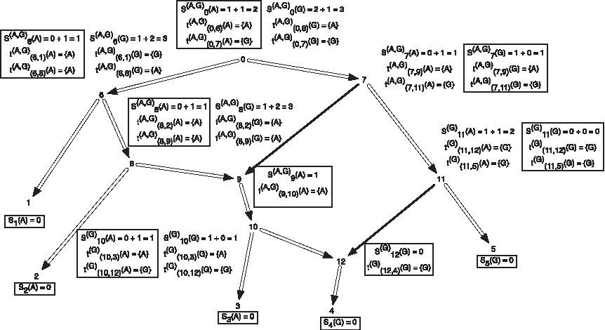
An example showing one among the at-most two dimensions of storage at each vertex of a phylogenetic network for computing the hardwired score and all optimal assignments on the network. The costs of each state at each node are shown next to the corresponding vertex; the cost matrix considered here is given by c_ij = 1 if i ≠ j and 0 if i = j for the states \documentclass{aastex}\usepackage{amsbsy}\usepackage{amsfonts}\usepackage{amssymb}\usepackage{bm}\usepackage{mathrsfs}\usepackage{pifont}\usepackage{stmaryrd}\usepackage{textcomp}\usepackage{portland, xspace}\usepackage{amsmath, amsxtra}\pagestyle{empty}\DeclareMathSizes{10}{9}{7}{6}\begin{document} $$i , j \in \{A , G \} $$ \end{document} . We order the reticulate vertices as (9, 12). The superscript (G) in S_v(.) at the vertices v = 10, 11, and 12 corresponds to the state G at the vertex 12, and the superscript (A,G) in S_v(.) at the vertices v = 0, 6, 7, 8, and 9 corresponds to the states at the reticulate vertices 9 and 12 respectively. Note that there is exactly one optimal assignment corresponding to the superscript (A, G), namely α(.), given by α(1) = A, α(2) = A, α(3) = A, α(4) = G, α(12) = G, α(10) = A, α(9) = A, α(8) = A, α(6) = A, α(5) = G, α(11) = G, α(7) = A, α(0) = A. This assignment can be obtained by preorder traversal of T_N, a spanning tree in N whose edges are shown in double arcs. The optimal assignment and its corresponding storage entries at each vertex are highlighted in boxes.

3.2. For softwired approach

Now we are ready to modify the above algorithm for the softwired approach. We need the following changes.

1) For the hardwired approach, T_N was fixed, and we used it for both vertex traversal of N and also for cost storage by using the reachability definition. For this approach, although we will still traverse the vertices of N via T_N for the storage of costs, we need to specify which parent of each reticulate vertex is used.

2) In the term \documentclass{aastex}\usepackage{amsbsy}\usepackage{amsfonts}\usepackage{amssymb}\usepackage{bm}\usepackage{mathrsfs}\usepackage{pifont}\usepackage{stmaryrd}\usepackage{textcomp}\usepackage{portland, xspace}\usepackage{amsmath, amsxtra}\pagestyle{empty}\DeclareMathSizes{10}{9}{7}{6}\begin{document} $$S_v^{( s_1 , s_2 , \ldots , s_t )} ( i )$$ \end{document} in the above algorithm, the parameters \documentclass{aastex}\usepackage{amsbsy}\usepackage{amsfonts}\usepackage{amssymb}\usepackage{bm}\usepackage{mathrsfs}\usepackage{pifont}\usepackage{stmaryrd}\usepackage{textcomp}\usepackage{portland, xspace}\usepackage{amsmath, amsxtra}\pagestyle{empty}\DeclareMathSizes{10}{9}{7}{6}\begin{document} $$s_1 , s_2 , \ldots , s_t$$ \end{document} represent the character states of the reticulate vertices \documentclass{aastex}\usepackage{amsbsy}\usepackage{amsfonts}\usepackage{amssymb}\usepackage{bm}\usepackage{mathrsfs}\usepackage{pifont}\usepackage{stmaryrd}\usepackage{textcomp}\usepackage{portland, xspace}\usepackage{amsmath, amsxtra}\pagestyle{empty}\DeclareMathSizes{10}{9}{7}{6}\begin{document} $$r_1 , r_2 , \ldots , r_t$$ \end{document} . In the softwired approach, \documentclass{aastex}\usepackage{amsbsy}\usepackage{amsfonts}\usepackage{amssymb}\usepackage{bm}\usepackage{mathrsfs}\usepackage{pifont}\usepackage{stmaryrd}\usepackage{textcomp}\usepackage{portland, xspace}\usepackage{amsmath, amsxtra}\pagestyle{empty}\DeclareMathSizes{10}{9}{7}{6}\begin{document} $$s_1 , s_2 , \ldots , s_t$$ \end{document} represent 0 or 1, depending on whether or not the left (first parent that is traversed) or the right (second parent that is traversed) parent of \documentclass{aastex}\usepackage{amsbsy}\usepackage{amsfonts}\usepackage{amssymb}\usepackage{bm}\usepackage{mathrsfs}\usepackage{pifont}\usepackage{stmaryrd}\usepackage{textcomp}\usepackage{portland, xspace}\usepackage{amsmath, amsxtra}\pagestyle{empty}\DeclareMathSizes{10}{9}{7}{6}\begin{document} $$v_1 , v_2 , \ldots , v_t$$ \end{document} are removed to calculate the costs of the subproblem. Note that the states \documentclass{aastex}\usepackage{amsbsy}\usepackage{amsfonts}\usepackage{amssymb}\usepackage{bm}\usepackage{mathrsfs}\usepackage{pifont}\usepackage{stmaryrd}\usepackage{textcomp}\usepackage{portland, xspace}\usepackage{amsmath, amsxtra}\pagestyle{empty}\DeclareMathSizes{10}{9}{7}{6}\begin{document} $$s_1 , s_2 , \ldots , s_t$$ \end{document} are different than the states i, j, which are character states.

The only place we need to make additional changes is in Subcase (ii), where we include a new function depending on whether the vertex v is traversed before the other reticulate parent of w_r, and if the left or the right parent is removed to construct the putative spanning tree.

3.2.1. Case 2

Subcase (ii): Without loss of generality, if w_r were a reticulate vertex r_q or the tail vertex d_q corresponding to a reticulate vertex r_q in T_N, then w_r appears in the list \documentclass{aastex}\usepackage{amsbsy}\usepackage{amsfonts}\usepackage{amssymb}\usepackage{bm}\usepackage{mathrsfs}\usepackage{pifont}\usepackage{stmaryrd}\usepackage{textcomp}\usepackage{portland, xspace}\usepackage{amsmath, amsxtra}\pagestyle{empty}\DeclareMathSizes{10}{9}{7}{6}\begin{document} $$n_1 , n_2 , \ldots , n_r$$ \end{document} . Without loss of generality, let n_z = r_q. Then, \documentclass{aastex}\usepackage{amsbsy}\usepackage{amsfonts}\usepackage{amssymb}\usepackage{bm}\usepackage{mathrsfs}\usepackage{pifont}\usepackage{stmaryrd}\usepackage{textcomp}\usepackage{portland, xspace}\usepackage{amsmath, amsxtra}\pagestyle{empty}\DeclareMathSizes{10}{9}{7}{6}\begin{document} \begin{align*} S_v^{( s_{c_1} , s_{c_2} , \ldots , s_{c_x}; s_{m_1} , s_{m_2} , \ldots , s_{m_y}; s_{n_1} , s_{n_2} , \ldots , s_{n_z} )} ( i ) = & min_j ( c_{ij}^{( v , w_l )} + S_{w_l}^{( s_{c_1} , s_{c_2} , \ldots , s_{c_x}; s_{m_1} , s_{m_2} , \ldots , s_{m_y} )} ( j ) ) \\ & + f ( w_r , s_{n_z} ) ( min_j ( c_{ij}^{( v , w_r )} + S_{r_q}^{( s_{c_1} , s_{c_2} , \ldots , s_{c_x}; s_{n_1} , s_{n_2} , \ldots , s_{n_z} )} ( j ) ) ) . & ( 5 ) \end{align*} \end{document}

where \documentclass{aastex}\usepackage{amsbsy}\usepackage{amsfonts}\usepackage{amssymb}\usepackage{bm}\usepackage{mathrsfs}\usepackage{pifont}\usepackage{stmaryrd}\usepackage{textcomp}\usepackage{portland, xspace}\usepackage{amsmath, amsxtra}\pagestyle{empty}\DeclareMathSizes{10}{9}{7}{6}\begin{document} \begin{align*}f ( w_r , s_{n_z} ) = \begin{cases} \chi_1 ( s_{n_z} ) \quad {\rm if} \ w_r = r_q; \\ \chi_0 ( s_{n_z} ) \quad {\rm if} \ w_r = d_q.\end{cases}\end{align*} \end{document}

and \documentclass{aastex}\usepackage{amsbsy}\usepackage{amsfonts}\usepackage{amssymb}\usepackage{bm}\usepackage{mathrsfs}\usepackage{pifont}\usepackage{stmaryrd}\usepackage{textcomp}\usepackage{portland, xspace}\usepackage{amsmath, amsxtra}\pagestyle{empty}\DeclareMathSizes{10}{9}{7}{6}\begin{document} \begin{align*}\chi_{a} ( s_{n_z} ) = \begin{cases}1 \quad {\rm if} \ s_{n_z} = a \\ 0 \quad {\rm otherwise}.\end{cases}\end{align*} \end{document}

Note that regardless of whether w_r = r_q or d_q, \documentclass{aastex}\usepackage{amsbsy}\usepackage{amsfonts}\usepackage{amssymb}\usepackage{bm}\usepackage{mathrsfs}\usepackage{pifont}\usepackage{stmaryrd}\usepackage{textcomp}\usepackage{portland, xspace}\usepackage{amsmath, amsxtra}\pagestyle{empty}\DeclareMathSizes{10}{9}{7}{6}\begin{document} $$S_{w_r}^{( s_{c_1} , s_{c_2} , \ldots , s_{c_x}; s_{n_1} , s_{n_2} , \ldots , s_{n_z} )} ( j $$ \end{document} ) is replaced by \documentclass{aastex}\usepackage{amsbsy}\usepackage{amsfonts}\usepackage{amssymb}\usepackage{bm}\usepackage{mathrsfs}\usepackage{pifont}\usepackage{stmaryrd}\usepackage{textcomp}\usepackage{portland, xspace}\usepackage{amsmath, amsxtra}\pagestyle{empty}\DeclareMathSizes{10}{9}{7}{6}\begin{document} $$S_{r_q}^{( s_{c_1} , s_{c_2} , \ldots , s_{c_x}; s_{n_1} , s_{n_2} , \ldots , s_{n_z} )} ( j $$ \end{document} ), and \documentclass{aastex}\usepackage{amsbsy}\usepackage{amsfonts}\usepackage{amssymb}\usepackage{bm}\usepackage{mathrsfs}\usepackage{pifont}\usepackage{stmaryrd}\usepackage{textcomp}\usepackage{portland, xspace}\usepackage{amsmath, amsxtra}\pagestyle{empty}\DeclareMathSizes{10}{9}{7}{6}\begin{document} $$S^{( i )}_{d_q} ( i )$$ \end{document} is never used. The way we handle (1) stated above is by using the function f (w_r, s_nz). It can also be seen that f (w_r, s_nz) can simply be written as \documentclass{aastex}\usepackage{amsbsy}\usepackage{amsfonts}\usepackage{amssymb}\usepackage{bm}\usepackage{mathrsfs}\usepackage{pifont}\usepackage{stmaryrd}\usepackage{textcomp}\usepackage{portland, xspace}\usepackage{amsmath, amsxtra}\pagestyle{empty}\DeclareMathSizes{10}{9}{7}{6}\begin{document} \begin{align*}f ( w_r , s_{n_z} ) = \chi_{\chi_{r_q} ( w_r )} ( s_{n_z} ).\end{align*} \end{document}

When performing the preorder traversal on T_N, any conflict assignments are ignored. In Figure 2, we present the subproblems of the hardwired approach for a character on a network. This set of subproblems also give multiple solutions as described in the figure.

FIG. 2.

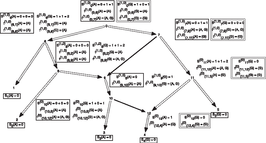
An example showing one among the at-most two dimensions of storage at each vertex of a phylogenetic network for computing the softwired score and all optimal assignments on the network. The costs of each state at each node are shown next to the corresponding vertex; the cost matrix considered here is given by c_ij = 1 if i ≠ j and 0 if i = j for the states \documentclass{aastex}\usepackage{amsbsy}\usepackage{amsfonts}\usepackage{amssymb}\usepackage{bm}\usepackage{mathrsfs}\usepackage{pifont}\usepackage{stmaryrd}\usepackage{textcomp}\usepackage{portland, xspace}\usepackage{amsmath, amsxtra}\pagestyle{empty}\DeclareMathSizes{10}{9}{7}{6}\begin{document} $$i , j \in \{A , G \} $$ \end{document} . We order the reticulate vertices as (9, 12). The superscript (0) in S_v(.) at the vertices v = 10, 11, and 12 corresponds to the state 0 at the vertex 12, which in turn corresponds to the deletion of the left edge (10, 12) incident at vertex 12 and the superscript (1, 0) in S_v(.) at the vertices v = 0, 6, 7, 8, and 9 corresponds to the states at the reticulate vertices 9 and 12 respectively, corresponding to the deletion of the right edge (7, 9) incident at vertex 9 and the left edge (11, 12) incident at vertex 12. Note that there are exactly three optimal assignments corresponding to the superscript (1, 0), namely α₁(.), α₂(.) and α₃(.) given by α₁(1) = A, α₁(2) = A, α₁(3) = A, α₁(4) = G, α₁(12) = G, α₁(10) = A, α₁(9) = A, α₁(8) = A, α₁(6) = A, α₁(5) = G, α₁(11) = G, α₁(7) = G, α₁(0) = G; α₂(1) = A, α₂(2) = A, α₂(3) = A, α₂(4) = G, α₂(12) = G, α₂(10) = A, α₂(9) = A, α₂(8) = A, α₂(6) = A, α₂(5) = G, α₂(11) = G, α₂(7) = G, α₂(0) = A and α₃(1) = A, α₃(2) = A, α₃(3) = A, α₃(4) = G, α₃(12) = G, α₃(10) = A, α₃(9) = A, α₃(8) = A, α₃(6) = A, α₃(5) = G, α₃(11) = G, α₃(7) = A, α₃(0) = A. These assignments can be obtained by preorder traversal of the spanning tree in N (whose edges are shown in double arcs) obtained by deleting the edges (7, 9) and (11, 12). The optimal assignments and its corresponding storage entries at each vertex are highlighted in boxes. Note that both the character states A and G are attained at the root vertex 0.

3.3. Problem complexity

Suppose p is the number of reticulate vertices in the network and k is the number of possible states of the character. Then we need O(k^p⁺¹) storage at each vertex for the hardwired approach and O(2^pk) for the softwired approach. If n is the number of leaves in N, by Lemma 2 there are O(n + p) vertices. Thus our algorithm requires O(m^rk(n + p)) storage, where n is the number of leaves and m = k for the hardwired approach and m = 2 for the softwired approach. Also by Theorem 3, p is at most n−2, thus rendering the total storage to O(m^pkn).

The tree traversal takes O(n), and to calculate the storage at a vertex, we need a calculation of O(k) for each of the O(km^pk) entries at each vertex. Thus the time complexity is O(nm^pk²). We note however that if all solutions were to be found, the preorder phase can be exponential, as is the case in Sankoff's algorithm.

3.3.1. Reduction step

We include the following clause to reduce storage and time complexity:

In case 2 of the algorithms, if y = z = 0, we have a special scenario in which both children w_l and w_r have exactly the same set of reticulate vertices that are reachable in T_N. When this occurs, we note that there is no subsequent vertex u in the postorder that is an ancestor of v, such that w is reachable from u. Suppose such a u exists, then one of the following holds, y = 1, z = 1, a contradiction. When this happens at a vertex v, the superscripts in \documentclass{aastex}\usepackage{amsbsy}\usepackage{amsfonts}\usepackage{amssymb}\usepackage{bm}\usepackage{mathrsfs}\usepackage{pifont}\usepackage{stmaryrd}\usepackage{textcomp}\usepackage{portland, xspace}\usepackage{amsmath, amsxtra}\pagestyle{empty}\DeclareMathSizes{10}{9}{7}{6}\begin{document} $$S_v^{( s_1 , s_2 , \ldots , s_t )} ( i )$$ \end{document} can be dropped and the storage is only O(k) at the vertex v, and the set of ( \documentclass{aastex}\usepackage{amsbsy}\usepackage{amsfonts}\usepackage{amssymb}\usepackage{bm}\usepackage{mathrsfs}\usepackage{pifont}\usepackage{stmaryrd}\usepackage{textcomp}\usepackage{portland, xspace}\usepackage{amsmath, amsxtra}\pagestyle{empty}\DeclareMathSizes{10}{9}{7}{6}\begin{document} $$s_1 , s_2 , \ldots , s_t$$ \end{document} )s that achieve the optimal S_v are also stored, whose storage is O(k^p). As a result, our algorithms are polynomial in time for networks whose reticulate cycles are disjoint, and in general if the number of intersecting cycles are bounded. See, for example, Figures 1 and 2.

4. Comparing Networks Based On Costs And Redundant Reticulate Vertices

In this section, we deal with comparing scores between networks. Although this is not part of the problem of finding the optimal score of a network, we show that there are some features in network score that can be directly relevant in comparing networks based on scores, which will be useful later for the problem of searching for networks with best scores.

4.1. Comparable scores across all networks

We first note that the cost of the softwired approach of a network is comparable with the softwired approach of any other network that has possibly different numbers of reticulate vertices compared to the original if the cost matrix is a metric by the argument below. For the softwired approach, the optimal score corresponds to a spanning tree in the network, which has 2n−2+2r edges by Lemma 2. Although, the number of edges in a phylogenetic tree is only 2n−2 since the costs along r edges are effectively omitted in the softwired cost, and by the triangle inequality, we notice that the states at the reticulate vertices must match either the states of the parents being used or the states of their child. Thus the network score has to be equal to that of the corresponding phylogenetic tree that can be constructed by contracting the edges incident to the reticulate vertices in the optimal spanning tree.

On the other hand, the hardwired score is not comparable across networks because of the differing quantity of edges in the network depending on the number of reticulate vertices present (namely, 2n− 2+3r). To address this fact, we adjust the score by subtracting, for each reticulate vertex, the maximum substitution cost across either of its incident reticulate edges. By doing this, we convert the score to that across only 2n−2+2r edges. Using the triangle inequality of the cost matrix, the network score is higher than that of the phylogenetic tree. Note that the network assignment might also not be an optimal assignment on the phylogenetic tree. Thus, we note that networks are penalized in this approach. We also present an interesting result below, namely, for binary states and unweighted costs (i.e., with cost matrix with diagonal entries zero and one elsewhere), the adjusted net score is the same as that of the softwired approach as shown in the result below.

Theorem 5: Let N be a network such that the reticulate cycles are edge-disjoint. Suppose we have a binary character and unweighted cost matrix. Let o_n and o_t be the cost of the network under the hardwired and the softwired approaches. Also, let adj(o_n) be the adjusted cost of o_n. Then adj(o_n) = o_t.

Proof:

We will prove the theorem for N with exactly one reticulate vertex. The general case can be proven by induction on the number of ret nodes.

The following are immediate:
i) adj(o_n) ≥ o_t

ii) o_n−1 ≤ adj(o_n) ≤ o_n,

iii) o_n−1 ≤ o_t ≤ o_n.

Case A: Suppose o_t = o_n.

By ii), adj(o_n) ≤ o_n = o_t. Thus, using i) and the above equation, we have adj(o_n) = o_t.

Case B: Suppose o_t = o_n−1.

Let α be an assignment on the nodes of N corresponding to softwired cost o_t. Let w be the reticulate node with parents p₁ and p₂, with p₂ not the parent of w in the optimum tree. Let c be the child of w.

Then without loss of generality (with 0 and 1 interchangeable), we have the following cases:
• α(p₁) = 0; α(r) = 0; α(c) = 0 or 1. Then α(p₂) = 1, for if α(p₂) = 0, then o_n = o_t, a contradiction to the assumption of the case. Thus α is also the optimal hardwired assignment o_n. Thus, adj(o_n) = o_n−1 = o_t.

• α(p₁) = 0 or 1; α(r) = 1; α(c) = 1. Then α(p₂) = 0, for if α(p₂) = 1, then o_n = o_t, a contradiction to the assumption of the case. Thus α is also a optimum hardwired assignment, and thus adj(o_n) = o_n−1 = o_t.

Note that α(p₁) = 0; α(r) = 1; α(c) = 0 is not possible, since α is an optimal softwired assignment. ■

Note that the above theorem is not extendable to general cost matrices or for nonbinary characters since we obtained counter-examples for these cases (that are not reported here). Thus in general, the adjusted hardwired score of a network is equal to or greater than the softwired score, and when they are equal, the number of solutions achieved by the adjusted hardwired approach is smaller than the number of solutions given by the softwired approach. For example, the adjusted hardwired cost of the network in Figure 1 is the same as its softwired cost of 1 (see Fig. 2). However, among the optimal softwired assignments α₁(.), α₂(.), and α₃(.), only α₁(.) and α₂(.) are optimal adjusted hardwired assignments.

4.2. Redundancy in reticulate nodes

Another ingredient in comparing networks is to be able to decide if the reticulate vertices are indeed needed. To check this, we make use of all solutions for the given problem. For a given optimal solution for a set of characters, we call a set of reticulate vertices R to be redundant if the solution does not use any of the reticulate vertices—that is, only a same parent of each vertex in R was used in the optimal spanning tree of all the characters. Thus the maximum number of redundant reticulate vertices can be computed by looking at all solutions of the characters formed by considering all combinations of solutions of the individual characters and computing the number of reticulate vertices that are redundant under each solution. Now, if the reticulate edge from the unused parent of a redundant vertex is removed, and any vertex of degree two is contracted, we will obtain a network with the same softwired cost and the same or lower hardwired cost. The list of unused parents can be computed immediately after the postorder traversal for the softwired approach; but only after the adjusted cost is computed (after the preorder traversal of finding all assignments) for the hardwired approach. Nevertheless, we need this computation only when we want to decrease or increase the number of reticulate vertices present.

In Figures 3 and 4, we give simple examples of when a tree is preferred and when a network with reticulate vertices is preferred for different datasets.

FIG. 3.
Example of a character dataset that displays a tree that models better than networks with reticulate vertices. The input set of three characters on two states “A” and “C” are given in the leaves. It can be seen that there is perfect phylogeny for this set of characters, namely, there is a tree (on the left) such that each of its internal edges splits a unique character into the two states (the edges that split the different characters are shown in dotted lines with the corresponding character site written next to each of them). Thus the tree is an optimal tree with parsimony cost of three, which equals the number of characters. Note that this is the minimum cost that can be attained for this dataset. Shown on the right is a network with the same input dataset. The softwired and adjusted hardwired parsimony costs of the network is three. However, it can be noted that the reticulate vertex 14 is redundant since the edge (13, 14) may be removed to render the same cost. In general, the network cost of this dataset on any network with at least one reticulate vertex will either have a cost of four or higher or if the score is three, then the set of all its reticulate vertices will be redundant. Thus the score on the left hand tree is better than the score on the right.

FIG. 4.
Example of two binary characters that are not compatible on a phylogenetic tree. Thus the parsimony score of the characters on any phylogenetic tree of six leaves has a cost of three or more. Shown in the figure is a network with one reticulate vertex with softwired and adjusted hardwired scores equal to two. This can be seen by the two dotted edges that allow one substitution each in different characters. While the first character has an additional substitution on the reticulate edge (11, 10), the second character has an additional substitution on the other reticulate edge (7, 10). Thus the two characters choose different optimal spanning trees (whose reticulate edges are shown in different colors with the corresponding character written next to them) inside the network, and the reticulate vertex 10 is not redundant. Hence, the score on this network is better than the score on any tree.

5. Testing A Real Dataset

We implemented our algorithm in OCAML, and it will be made available in the upcoming versions of the POY software (Varón et al., 2010). In order to see how our algorithm performs, we tested it on real sequence data collected from ant species complex in which hybridization could be common. Hybridization events have been observed in the evolutionary histories of ants belonging to various genera, such as Formica (Seifert et al., 2010) and Dorylus (Kronauer et al., 2011). We chose a fraction of a dataset taken from the Camponotus maculatus species complex, the full version of which will appear in Clouse et al. (2010). The dataset consisted of a marker each from the nucleus (LR, long wavelength rhodopsin) and mitochondrion (COI, cytochrome c oxidase I) from 82 specimens collected throughout the Indo-Pacific. The data gathered was reduced to a manageable size by first conducting tree searches in POY (Varón et al., 2010) for the two markers separately. The sequences of 57 taxa showed clear conflict in phylogenetic placement or were needed to establish the main lineages in the complex retained in the dataset. The mitocondrial and the nuclear sequences were aligned and concatenated. As shown in Table 1, the softwired parsimony cost of the network shown in Figure 5 that was formed by adding two reticulate vertices to the most parsimonious tree formed from nuclear sequences was lower than the sum of the best parsimony scores of the individual mitochondrial and nuclear sequences. This network was compared against other random networks with two reticulate vertices for costs and by far has the lowest hardwired and softwired cost. While it is expected that with the addition of more and more reticulate vertices, the softwired cost will not be lesser compared to the tree cost, we did not see any decrease in cost as we added more than two reticulate vertices. Additionally, we identified redundant reticulate vertices in all the random networks we generated with three or more reticulate vertices. Also shown in the table are the hardwired costs with the adjusted scores in parenthesis. Although the hardwired scores and their adjusted scores are higher than the softwired costs for the network, the given network has the best hardwired cost among all the phylogenetic networks with two or more reticulate vertices that we considered. In both the approaches, the network did not have any redundant vertices.

FIG. 5.
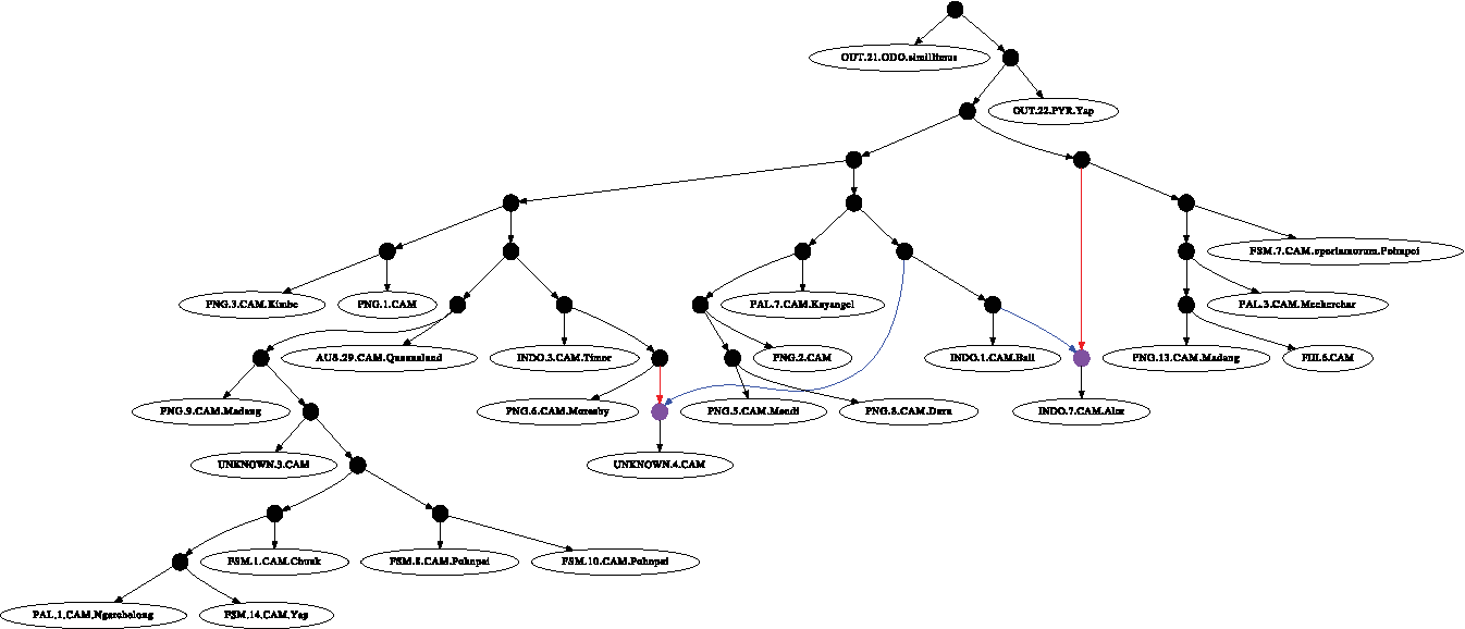
Experimental real data showing hybridization events in the Camponotus maculatus species complex. The blue and red edges correspond to the spanning trees that are most parsimonious to most characters in the LR and COI markers respectively.

Table 1.
Parsimony Scores of the Network Shown in Figure 5

(i) (ii) (iii) (iv) (v)

Mitocondrial 477 745 746 907 (789)

Nuclear 560 1942 1915 2095 (1945)

Total 1037 2687 2661 3002 (2734)

Aligned mitocondrial and nuclear sequences of 57 taxa taken from Camponotus maculatus species: (i) Sequence type; (ii) length of sequence; (iii) tree cost; (iv) softwired network cost; and (v) hardwired network cost (adjusted cost).

While the softwired score can be used to compare networks directly, the hardwired scores can only be used to compare networks with the same number of reticulate vertices. In both the approaches, the number of reticulate vertices must be checked for redundancy. This will help place a bound on the number of reticulate vertices that we allow in the networks.

6. Conclusion

In this article, we provided a dynamic programming solution to compute exactly the hardwired and softwired parsimony scores on phylogenetic networks. As opposed to the hardwired approach, the subproblems that we consider for the softwired approach are finding the costs of each state at each vertex for each subgraph by removing one reticulate edge each of the reticulate vertices reachable from the vertex. We showed that although the subproblems are different, they can both be solved by the dynamic programming approach using the same vertex traversal order. We also gave a reduction step that reduces both the storage and time complexities of the algorithms.

We noticed that the two approaches have some properties that suggest the existence of simpler algorithms. First, for binary states and binary cost-matrix, the softwired and hardwired scores are the same; although, the number of solutions can differ. It is well known that the hardwired problem is polynomially solvable. It would be interesting to derive a polynomial algorithm for the softwired approach as well. Second, for planar graph and binary cost-matrix, it has been proven in Hartvigsen (1998) that the hardwired problem is polynomially solvable. It would thus be possible to obtain an algorithm for computing the hardwired score on phylogenetic networks, perhaps similar to the Fitch algorithm (Fitch, 1971) for phylogenetic trees. Note that by Lemma 1, the networks that we consider are planar.

The algorithms provide us with the states at the reticulate vertices that fetch the optimal assignments. For the softwired approach, this readily gives us a method to realize if a set of vertices are redundant. Maximizing the size of the redundant networks helps us to realize a network with a minimum number of reticulate vertices. For the hardwired approach, we provide a method to adjust the cost by removing a reticulate edge for each reticulate vertex that has the highest traversal cost. This gives a score that is comparable across different networks with different vertices, a feature that is readily available in the softwired approach. Additionally, redundancy can also be incorporated in the hardwired approach after the adjusted scores are found. Thus, we provide a method to compare network cost to navigate through the space of networks. We also note that although the softwired approach in theory is more challenging to tackle, we have a faster exact algorithm for this approach that readily gives a method to compare networks based on the cost and also the number of redundant reticulate vertices. Methods such as these will help search for the best networks with an optimum number of reticulate vertices, the next major challenge that needs to be addressed to find the “Net of Life.”

(i)	(ii)	(iii)	(iv)	(v)
Mitocondrial	477	745	746	907 (789)
Nuclear	560	1942	1915	2095 (1945)
Total	1037	2687	2661	3002 (2734)

Footnotes

Acknowledgments

We thank Nicolas Lucaroni for suggestions provided while implementing the algorithms. We sincerely thank Ronald Clouse and Milan Janda for Camponotus sequence data, which were collected with the following support: DARPA (W911NF-05-1-0271); Marie Currie Fellowship (PIOFGA2009-25448); Czech Science Foundation (P505/10/0673; 206/09/0115); Czech Ministry of Education Grants (LC06073; 6007665801); and Putnam Expedition Grants (Museum of Comparative Zoology). We also thank Anupam Kumar and Sameer Siddiqi, who filtered the dataset to a manageable size. This material is based upon work supported by, or in part by, the U.S. Army Research Laboratory and the U.S. Army Research Office under grant number W911NF- 05-1-0271.

Author Disclosure Statement

The authors declare that no competing financial interests exist.

References

Clouse

R.M.

, Janda

, Blanchard

, et al. 2013. Camponotus maculatus-group ants and biogeographic heterogeneity in the indo-pacific. (manuscript in preparation.)

Dahlhaus

, Johnson

D.S.

, Papadimitriou

C.H.

, et al. 1994. The complexity of multiterminal cuts. SIAM Journal on Computing, 23, 864–894.

Edwards

A.W.F.

, and Cavalli-Sforza

L.L.

1963. The reconstruction of evolution. Annals of Human Genetics (also published in Heredity 18, 553), 27, 105–106.

Erdös

P.L.

, and Székely

L.A.

1994. On weighted multiway cuts in trees. Math. Program., 65, 93–105.

Farris

J.S.

1966. Estimation of conservatism of characters by constancy within biological populations. Evolution, 20, pp. 587–591.

Fisher

, Van Iersel

, Kelk

, et al. 2013. On computing the maximum parsimony score of a phylogenetic network. Available at: http://arxiv.org/abs/1302.2430

Fitch

W.M.

, 1971. Toward defining the course of evolution: Minimum change for a specific tree topology. Systematic Zoology, 20, 406–416.

Hartvigsen

1998. The planar multiterminal cut problem. Discrete Applied Mathematics, 85, 203–222.

Huson

D.H.

, Rupp

, and Scornavacca

2011. Phylogenetic Networks: Concepts, Algorithms and Applications. Cambridge University Press, Cambridge, United Kingdom.

10.

Kannan

, and Wheeler

W.C.

2012. Maximum parsimony on phylogenetic networks. Algorithms Mol Biol., 7, 9.

11.

Kluge

A.G.

, and Farris

J.S.

1969. Quantitative Phyletics and the Evolution of Anurans. Systematic Zoology. 18.

12.

Kronauer

, Peters

, Schoning

, et al. 2011. Hybridization in East African swarm-raiding army ants. Frontiers in Zoology, 8, 20.

13.

Moret

B.M.

, Nakhleh

, Warnow

, et al. 2004. Phylogenetic networks: modeling, reconstructibility, and accuracy. IEEE/ACM Trans. Comput. Biol. Bioinform., 1, 13–23.

14.

Nakhleh

, Jin

, Zhao

, et al. 2005. Reconstructing phylogenetic networks using maximum parsimony. Proceedings of the 2005 IEEE Computational Systems Bioinformatics Conference, 93–102.

15.

Sankoff

1975. Minimal mutation trees of sequences. SIAM Journal of Applied Mathematics, 28, 3542.

16.

Sankoff

, and Rousseau

1975. Locating the vertices of a Steiner tree in an arbitrary metric space. Math. Progr., 9, 240–276.

17.

Schrijver

2003. Combinatorial Optimization - Polyhedra and Efficiency. Springer.

18.

Seifert

, Kulmuni

, and Pamilo

2010. Independent hybrid populations of formica polyctena xrufa wood ants (hymenoptera: Formicidae) abound under conditions of forest fragmentation. Evolutionary Ecology.

19.

Tuffley

, and Steel

1997. Links between maximum likelihood and maximum parsimony under a simple model of site substitution. Bulletin of Mathematical Biology, 59, 581–607.

20.

Varón

, Vinh

L.S.

, and Wheeler

W.C.

2010. Poy version 4: phylogenetic analysis using dynamic homologies. Cladistics, 26, 72–85.

Exactly Computing the Parsimony Scores on Phylogenetic Networks Using Dynamic Programming

Abstract

Abstract

1. Introduction

1.1. Maximum parsimony on networks

1.2. Dynamic programming

2. Preliminaries

2.1. Phylogenetic networks

Lemma 1

Proof

Lemma 2

Theorem 3

Proof (by induction on nv)

Theorem 4

Proof (by induction on n:)

2.2. Tree representation of a network

2.3. Parsimony score

2.4. Network traversal

3. Computing Parsimony Score With The Dynamic Programming Approach

3.1. For the hardwired approach

3.2. For softwired approach

3.2.1. Case 2

3.3. Problem complexity

3.3.1. Reduction step

4. Comparing Networks Based On Costs And Redundant Reticulate Vertices

4.1. Comparable scores across all networks

Proof:

4.2. Redundancy in reticulate nodes

5. Testing A Real Dataset

6. Conclusion

Footnotes

Acknowledgments

Author Disclosure Statement

References

Proof (by induction on n_v)