In this article we explain how to easily compute gene clusters, formalized by classical or generalized nested common or conserved intervals, between a set of K genomes represented as K permutations. A b-nested common (resp. conserved) interval I of size |I| is either an interval of size 1 or a common (resp. conserved) interval that contains another b-nested common (resp. conserved) interval of size at least |I|−b. When b = 1, this corresponds to the classical notion of nested interval. We exhibit two simple algorithms to output all b-nested common or conserved intervals between K permutations in O(Kn + nocc) time, where nocc is the total number of such intervals. We also explain how to count all b-nested intervals in O(Kn) time. New properties of the family of conserved intervals are proposed to do so.
1. Introduction
Comparative genomics is nowadays a classical field in computational biology, and one of its typical problems is to cluster sets of orthologous genes that have virtually the same function in several genomes. A very strong paradigm is that groups of genes that remain “close” during evolution work together (see, for instance, Galperin and Koonin, 2000, Lathe et al., 2000, Tamames, 2001). Thus, a widely used approach to obtain interesting clusters is to try to cluster genes or other biological units (for instance, unique contigs of protein domains) according to their common proximity on several genomes. For this goal, many different cluster models have been proposed, like common intervals in Uno and Yagiura (2000), conserved intervals in Bergeron et al. (2004), π-patterns in Parida (2006), gene teams in Béal et al. (2004), domain teams in Pasek et al. (2005), approximate common intervals in Amir et al. (2007) and so on, considering different chromosome models (permutations, signed permutations, sequences, graphs, etc.) or different distance models (accepting gaps, distance modeled as weighted graphs, etc.)
Among all those models, the first proposed, and still one of the most used in practice, is the concept of common interval on genomes represented by permutations. A set of genes form a common interval of K genomes if it appears as a segment on each of the K unsigned permutations that represent the genomes. The orders inside the segments might be totally different. The model of conserved interval is close to the model of common interval but considers signed permutations.
Recently, nested common intervals (easily extensible to nested conserved intervals) were introduced in Hoberman and Durand (2005) based on real data observation by Kurzik-Dumke and Zengerle (1996). A common interval I of size |I| is nested if |I| = 1 or if it contains at least one nested common interval of size |I|−1. Hoberman and Durand (2005) pointed out that the nestedness assumption can strengthen the significance of detected clusters since it reduces the probability of observing them randomly. An O(n2) time algorithm to compute all nested common intervals between two permutations has been presented in Blin et al. (2010) while, between K permutations, a recent O(Kn + nocc) algorithm is proposed in Rusu (2013), where nocc is the number of solutions.
In this article, we exhibit two simple algorithms to easily compute nested common and conserved intervals of K permutations from their natural tree representations. Also, with the same simplicity, we propose to deal with a generalization of nested common intervals, called b-nested common intervals, and with its variant for conserved intervals (which are a signed version of common intervals), called b-nested conserved intervals. These new classes allow—as b grows—for a less constraint containment between the intervals in the family. Indeed, a nested interval I must contain a nested interval of size |I|−1 or be a unit interval. A b-nested common (resp. conserved) interval must contain a b-nested common (resp. conserved) interval of size at least |I|− b or be a unit interval. Nested intervals are indead 1-nested. From a biological point of view, this is equivalent to modeling clusters with a larger variability in gene content and gene order, thus allowing algorithms to deal with annotation errors. However, the study and validation of this new interval model is deferred to further applied studies. In this article we focus on the algorithmic aspects.
Given a set \documentclass{aastex}\usepackage{amsbsy}\usepackage{amsfonts}\usepackage{amssymb}\usepackage{bm}\usepackage{mathrsfs}\usepackage{pifont}\usepackage{stmaryrd}\usepackage{textcomp}\usepackage{portland, xspace}\usepackage{amsmath, amsxtra}\pagestyle{empty}\DeclareMathSizes{10}{9}{7}{6}\begin{document}
$${\cal P}$$
\end{document} of K permutations on n elements representing genomes with no duplicates, our simple algorithms for finding all b-nested common or conserved intervals of \documentclass{aastex}\usepackage{amsbsy}\usepackage{amsfonts}\usepackage{amssymb}\usepackage{bm}\usepackage{mathrsfs}\usepackage{pifont}\usepackage{stmaryrd}\usepackage{textcomp}\usepackage{portland, xspace}\usepackage{amsmath, amsxtra}\pagestyle{empty}\DeclareMathSizes{10}{9}{7}{6}\begin{document}
$${\cal P}$$
\end{document} run in O(Kn + nocc)-time and need O(n) additional space, where nocc is the number of solutions. In this way, our algorithm for common intervals performs as well as the algorithm in Rusu (2013) for the case of K permutations and proposes an efficient approach for the new classes of b-nested intervals.
Moreover, a slight modification of our approach allows us to count the number of b-nested common or conserved intervals of K permutations in O(Kn) time. Efficiently counting the number of b-nested common intervals without enumerating them is very useful when one needs to compute similarity functions between genomes that are expressed in terms of number of intervals (see, for instance, Fertin and Rusu, 2011).
The article is organized as follows. In Section 2, we present the main definitions for common and conserved intervals and precisely state the problem to solve. In Section 3, we focus on b-nested common intervals, recalling the data structure called a PQ-tree, giving a characterization of b-nested common intervals and showing how PQ-trees can be used to find all b-nested common intervals. In Section 4, we adopt a similar approach for conserved intervals, with the difference that another tree structure must be used in this case. In Section 5, we discuss our conclusion.
2. Generalities on Common and Conserved Intervals
A permutation P on n elements is a complete linear order on the set of integers \documentclass{aastex}\usepackage{amsbsy}\usepackage{amsfonts}\usepackage{amssymb}\usepackage{bm}\usepackage{mathrsfs}\usepackage{pifont}\usepackage{stmaryrd}\usepackage{textcomp}\usepackage{portland, xspace}\usepackage{amsmath, amsxtra}\pagestyle{empty}\DeclareMathSizes{10}{9}{7}{6}\begin{document}
$$\{1 , 2 , \ldots , n \} $$
\end{document}. We denote Idn the identity permutation (\documentclass{aastex}\usepackage{amsbsy}\usepackage{amsfonts}\usepackage{amssymb}\usepackage{bm}\usepackage{mathrsfs}\usepackage{pifont}\usepackage{stmaryrd}\usepackage{textcomp}\usepackage{portland, xspace}\usepackage{amsmath, amsxtra}\pagestyle{empty}\DeclareMathSizes{10}{9}{7}{6}\begin{document}
$$1 , 2 , \ldots , n$$
\end{document}). An interval of a permutation \documentclass{aastex}\usepackage{amsbsy}\usepackage{amsfonts}\usepackage{amssymb}\usepackage{bm}\usepackage{mathrsfs}\usepackage{pifont}\usepackage{stmaryrd}\usepackage{textcomp}\usepackage{portland, xspace}\usepackage{amsmath, amsxtra}\pagestyle{empty}\DeclareMathSizes{10}{9}{7}{6}\begin{document}
$$P = ( p_1 , p_2 , \ldots , p_n )$$
\end{document} is a set of consecutive elements of the permutation P. An interval of a permutation will be denoted by giving its first and last positions, such as [i, j]. Such an interval is also said delimited by pi (left) and pj (right). An interval \documentclass{aastex}\usepackage{amsbsy}\usepackage{amsfonts}\usepackage{amssymb}\usepackage{bm}\usepackage{mathrsfs}\usepackage{pifont}\usepackage{stmaryrd}\usepackage{textcomp}\usepackage{portland, xspace}\usepackage{amsmath, amsxtra}\pagestyle{empty}\DeclareMathSizes{10}{9}{7}{6}\begin{document}
$$[ i , j ] = \{i , i + 1 , \ldots , j \} $$
\end{document} of the identity permutation will be simply denoted by (i.j).
Let\documentclass{aastex}\usepackage{amsbsy}\usepackage{amsfonts}\usepackage{amssymb}\usepackage{bm}\usepackage{mathrsfs}\usepackage{pifont}\usepackage{stmaryrd}\usepackage{textcomp}\usepackage{portland, xspace}\usepackage{amsmath, amsxtra}\pagestyle{empty}\DeclareMathSizes{10}{9}{7}{6}\begin{document}
$${\cal P} = \{P_1 , P_2 , \ldots , P_K \} $$
\end{document}be a set of K permutations on n elements. A common interval of\documentclass{aastex}\usepackage{amsbsy}\usepackage{amsfonts}\usepackage{amssymb}\usepackage{bm}\usepackage{mathrsfs}\usepackage{pifont}\usepackage{stmaryrd}\usepackage{textcomp}\usepackage{portland, xspace}\usepackage{amsmath, amsxtra}\pagestyle{empty}\DeclareMathSizes{10}{9}{7}{6}\begin{document}
$${\cal P}$$
\end{document}is a set of integers that is an interval in each permutation of\documentclass{aastex}\usepackage{amsbsy}\usepackage{amsfonts}\usepackage{amssymb}\usepackage{bm}\usepackage{mathrsfs}\usepackage{pifont}\usepackage{stmaryrd}\usepackage{textcomp}\usepackage{portland, xspace}\usepackage{amsmath, amsxtra}\pagestyle{empty}\DeclareMathSizes{10}{9}{7}{6}\begin{document}
$${\cal P}$$
\end{document}.
The set \documentclass{aastex}\usepackage{amsbsy}\usepackage{amsfonts}\usepackage{amssymb}\usepackage{bm}\usepackage{mathrsfs}\usepackage{pifont}\usepackage{stmaryrd}\usepackage{textcomp}\usepackage{portland, xspace}\usepackage{amsmath, amsxtra}\pagestyle{empty}\DeclareMathSizes{10}{9}{7}{6}\begin{document}
$$\{1 , 2 , \ldots , n \} $$
\end{document} and all singletons (also called unit intervals) are common intervals of any non-empty set \documentclass{aastex}\usepackage{amsbsy}\usepackage{amsfonts}\usepackage{amssymb}\usepackage{bm}\usepackage{mathrsfs}\usepackage{pifont}\usepackage{stmaryrd}\usepackage{textcomp}\usepackage{portland, xspace}\usepackage{amsmath, amsxtra}\pagestyle{empty}\DeclareMathSizes{10}{9}{7}{6}\begin{document}
$${\cal P}$$
\end{document} of permutations. Moreover, one can always assume that one of the permutations, say P1, is the identity permutation Idn. For this, it is sufficient to renumber the elements of P1 so as to obtain Idn, and then to renumber all the other permutations accordingly. Then the common intervals of \documentclass{aastex}\usepackage{amsbsy}\usepackage{amsfonts}\usepackage{amssymb}\usepackage{bm}\usepackage{mathrsfs}\usepackage{pifont}\usepackage{stmaryrd}\usepackage{textcomp}\usepackage{portland, xspace}\usepackage{amsmath, amsxtra}\pagestyle{empty}\DeclareMathSizes{10}{9}{7}{6}\begin{document}
$${\cal P}$$
\end{document} are of the form (i.j) with 1 ≤ i ≤ j ≤ n.
Define now a signed permutation as a permutation P whose elements have an associated sign among + and −, making each element to be respectively positive or negative. Negative elements are denoted −pi while positive elements are simply denoted pi, or +pi for emphasizing positivity. A permutation is then a signed permutation containing only positive elements.
Let\documentclass{aastex}\usepackage{amsbsy}\usepackage{amsfonts}\usepackage{amssymb}\usepackage{bm}\usepackage{mathrsfs}\usepackage{pifont}\usepackage{stmaryrd}\usepackage{textcomp}\usepackage{portland, xspace}\usepackage{amsmath, amsxtra}\pagestyle{empty}\DeclareMathSizes{10}{9}{7}{6}\begin{document}
$${\cal P} = \{P_1 , P_2 , \ldots , P_K \} $$
\end{document}be a set of signed permutations over\documentclass{aastex}\usepackage{amsbsy}\usepackage{amsfonts}\usepackage{amssymb}\usepackage{bm}\usepackage{mathrsfs}\usepackage{pifont}\usepackage{stmaryrd}\usepackage{textcomp}\usepackage{portland, xspace}\usepackage{amsmath, amsxtra}\pagestyle{empty}\DeclareMathSizes{10}{9}{7}{6}\begin{document}
$$\{1 , 2 , \ldots , n \} $$
\end{document}, with first element + 1 and last element + n, for each\documentclass{aastex}\usepackage{amsbsy}\usepackage{amsfonts}\usepackage{amssymb}\usepackage{bm}\usepackage{mathrsfs}\usepackage{pifont}\usepackage{stmaryrd}\usepackage{textcomp}\usepackage{portland, xspace}\usepackage{amsmath, amsxtra}\pagestyle{empty}\DeclareMathSizes{10}{9}{7}{6}\begin{document}
$$k \in \{1 , 2 , \ldots , K \} $$
\end{document}. Assume P1 = Idn. A conserved interval of\documentclass{aastex}\usepackage{amsbsy}\usepackage{amsfonts}\usepackage{amssymb}\usepackage{bm}\usepackage{mathrsfs}\usepackage{pifont}\usepackage{stmaryrd}\usepackage{textcomp}\usepackage{portland, xspace}\usepackage{amsmath, amsxtra}\pagestyle{empty}\DeclareMathSizes{10}{9}{7}{6}\begin{document}
$${\cal P}$$
\end{document}is either a unit interval or a common interval (a.c) of\documentclass{aastex}\usepackage{amsbsy}\usepackage{amsfonts}\usepackage{amssymb}\usepackage{bm}\usepackage{mathrsfs}\usepackage{pifont}\usepackage{stmaryrd}\usepackage{textcomp}\usepackage{portland, xspace}\usepackage{amsmath, amsxtra}\pagestyle{empty}\DeclareMathSizes{10}{9}{7}{6}\begin{document}
$${\cal P}$$
\end{document}(ignoring the signs), which is delimited in each Pk either by a (left) and c (right), or by −c (left) and −a (right).
Remark 1
In the remaining of the paper, we assume that \documentclass{aastex}\usepackage{amsbsy}\usepackage{amsfonts}\usepackage{amssymb}\usepackage{bm}\usepackage{mathrsfs}\usepackage{pifont}\usepackage{stmaryrd}\usepackage{textcomp}\usepackage{portland, xspace}\usepackage{amsmath, amsxtra}\pagestyle{empty}\DeclareMathSizes{10}{9}{7}{6}\begin{document}
$${\cal P} = \{P_1 , P_2 , \ldots , P_K \} $$
\end{document} with P1 = Idn. Moreover, when we deal with conserved intervals, the permutations are assumed to satisfy the hypothesis in Definition 2.
Now, we are ready to introduce the new classes of intervals.
Definition 3
Let\documentclass{aastex}\usepackage{amsbsy}\usepackage{amsfonts}\usepackage{amssymb}\usepackage{bm}\usepackage{mathrsfs}\usepackage{pifont}\usepackage{stmaryrd}\usepackage{textcomp}\usepackage{portland, xspace}\usepackage{amsmath, amsxtra}\pagestyle{empty}\DeclareMathSizes{10}{9}{7}{6}\begin{document}
$${\cal P} = \{P_1 , P_2 , \ldots , P_K \} $$
\end{document}be a set of K permutations on n elements, and let b be a positive integer. A common (resp. conserved) interval of\documentclass{aastex}\usepackage{amsbsy}\usepackage{amsfonts}\usepackage{amssymb}\usepackage{bm}\usepackage{mathrsfs}\usepackage{pifont}\usepackage{stmaryrd}\usepackage{textcomp}\usepackage{portland, xspace}\usepackage{amsmath, amsxtra}\pagestyle{empty}\DeclareMathSizes{10}{9}{7}{6}\begin{document}
$${\cal P}$$
\end{document}is b-nested if either |I| = 1 or I strictly contains a common (resp. conserved) interval of size at least |I|−b.
We are interested in efficient algorithms for finding and counting all b-nested common (resp. conserved) intervals of \documentclass{aastex}\usepackage{amsbsy}\usepackage{amsfonts}\usepackage{amssymb}\usepackage{bm}\usepackage{mathrsfs}\usepackage{pifont}\usepackage{stmaryrd}\usepackage{textcomp}\usepackage{portland, xspace}\usepackage{amsmath, amsxtra}\pagestyle{empty}\DeclareMathSizes{10}{9}{7}{6}\begin{document}
$${\cal P} = \{P_1 , P_2 , \ldots , P_K \} $$
\end{document}, without redundancy. Obviously, unit intervals are, by definition, b-nested common (resp. conserved) intervals. As a consequence, from now on and without any subsequent specification, we focus on finding b-nested common (resp. conserved) intervals of size at least 2. The following notions will be very useful in the subsequent.
Definition 4
Let\documentclass{aastex}\usepackage{amsbsy}\usepackage{amsfonts}\usepackage{amssymb}\usepackage{bm}\usepackage{mathrsfs}\usepackage{pifont}\usepackage{stmaryrd}\usepackage{textcomp}\usepackage{portland, xspace}\usepackage{amsmath, amsxtra}\pagestyle{empty}\DeclareMathSizes{10}{9}{7}{6}\begin{document}
$${\cal P} = \{P_1 , P_2 , \ldots , P_K \} $$
\end{document}be a set of K permutations on n elements and let b be a positive integer. A common (resp. conserved) interval of\documentclass{aastex}\usepackage{amsbsy}\usepackage{amsfonts}\usepackage{amssymb}\usepackage{bm}\usepackage{mathrsfs}\usepackage{pifont}\usepackage{stmaryrd}\usepackage{textcomp}\usepackage{portland, xspace}\usepackage{amsmath, amsxtra}\pagestyle{empty}\DeclareMathSizes{10}{9}{7}{6}\begin{document}
$${\cal P}$$
\end{document}is b-small if its size does not exceed b. Otherwise, the interval is b-large. Notice that all b-small intervals are b-nested by definition and since unit intervals are b-nested.
3. on b-nested Common Intervals
This section is divided into three parts. The first one recalls a tree structure that we associate with common intervals of permutations, the PQ-trees. The second one discusses the properties of b-nested common intervals. Finally, we give the algorithms for efficiently computing and counting the b-nested common intervals.
3.1. PQ-trees and common intervals
Definition 5
Let\documentclass{aastex}\usepackage{amsbsy}\usepackage{amsfonts}\usepackage{amssymb}\usepackage{bm}\usepackage{mathrsfs}\usepackage{pifont}\usepackage{stmaryrd}\usepackage{textcomp}\usepackage{portland, xspace}\usepackage{amsmath, amsxtra}\pagestyle{empty}\DeclareMathSizes{10}{9}{7}{6}\begin{document}
$${\cal F}$$
\end{document}be a family of intervals from Idn containing the interval (1.n). A PQ-tree representing the family \documentclass{aastex}\usepackage{amsbsy}\usepackage{amsfonts}\usepackage{amssymb}\usepackage{bm}\usepackage{mathrsfs}\usepackage{pifont}\usepackage{stmaryrd}\usepackage{textcomp}\usepackage{portland, xspace}\usepackage{amsmath, amsxtra}\pagestyle{empty}\DeclareMathSizes{10}{9}{7}{6}\begin{document}
$${\cal F}$$
\end{document}is a tree T(\documentclass{aastex}\usepackage{amsbsy}\usepackage{amsfonts}\usepackage{amssymb}\usepackage{bm}\usepackage{mathrsfs}\usepackage{pifont}\usepackage{stmaryrd}\usepackage{textcomp}\usepackage{portland, xspace}\usepackage{amsmath, amsxtra}\pagestyle{empty}\DeclareMathSizes{10}{9}{7}{6}\begin{document}
$${\cal F}$$
\end{document}) satisfying the following:
1. Its nodes are in bijection with a subset S(\documentclass{aastex}\usepackage{amsbsy}\usepackage{amsfonts}\usepackage{amssymb}\usepackage{bm}\usepackage{mathrsfs}\usepackage{pifont}\usepackage{stmaryrd}\usepackage{textcomp}\usepackage{portland, xspace}\usepackage{amsmath, amsxtra}\pagestyle{empty}\DeclareMathSizes{10}{9}{7}{6}\begin{document}
$${\cal F}$$
\end{document}) of intervals from\documentclass{aastex}\usepackage{amsbsy}\usepackage{amsfonts}\usepackage{amssymb}\usepackage{bm}\usepackage{mathrsfs}\usepackage{pifont}\usepackage{stmaryrd}\usepackage{textcomp}\usepackage{portland, xspace}\usepackage{amsmath, amsxtra}\pagestyle{empty}\DeclareMathSizes{10}{9}{7}{6}\begin{document}
$${\cal F}$$
\end{document}, the root corresponding to (1.n).
2. Its arcs represent all the direct (not obtained by transitivity) inclusions between intervals in S(\documentclass{aastex}\usepackage{amsbsy}\usepackage{amsfonts}\usepackage{amssymb}\usepackage{bm}\usepackage{mathrsfs}\usepackage{pifont}\usepackage{stmaryrd}\usepackage{textcomp}\usepackage{portland, xspace}\usepackage{amsmath, amsxtra}\pagestyle{empty}\DeclareMathSizes{10}{9}{7}{6}\begin{document}
$${\cal F}$$
\end{document}).
3. Each node is labeled P or Q, and an order is defined for the children of each Q-node
4. An interval I of Idn belongs to\documentclass{aastex}\usepackage{amsbsy}\usepackage{amsfonts}\usepackage{amssymb}\usepackage{bm}\usepackage{mathrsfs}\usepackage{pifont}\usepackage{stmaryrd}\usepackage{textcomp}\usepackage{portland, xspace}\usepackage{amsmath, amsxtra}\pagestyle{empty}\DeclareMathSizes{10}{9}{7}{6}\begin{document}
$${\cal F}$$
\end{document}iff either it corresponds to a node or there exists a unique Q-node z such that I is the union of intervals corresponding to successive children of z, according to the order defined for z.
Note that the size of the tree is in \documentclass{aastex}\usepackage{amsbsy}\usepackage{amsfonts}\usepackage{amssymb}\usepackage{bm}\usepackage{mathrsfs}\usepackage{pifont}\usepackage{stmaryrd}\usepackage{textcomp}\usepackage{portland, xspace}\usepackage{amsmath, amsxtra}\pagestyle{empty}\DeclareMathSizes{10}{9}{7}{6}\begin{document}
$$O ( \mid S ( {\cal F} ) \mid )$$
\end{document}, thus allowing to drastically reduce the memory space needed to store all the intervals in \documentclass{aastex}\usepackage{amsbsy}\usepackage{amsfonts}\usepackage{amssymb}\usepackage{bm}\usepackage{mathrsfs}\usepackage{pifont}\usepackage{stmaryrd}\usepackage{textcomp}\usepackage{portland, xspace}\usepackage{amsmath, amsxtra}\pagestyle{empty}\DeclareMathSizes{10}{9}{7}{6}\begin{document}
$${\cal F}$$
\end{document}. When labels P and Q are forgotten, the tree T(\documentclass{aastex}\usepackage{amsbsy}\usepackage{amsfonts}\usepackage{amssymb}\usepackage{bm}\usepackage{mathrsfs}\usepackage{pifont}\usepackage{stmaryrd}\usepackage{textcomp}\usepackage{portland, xspace}\usepackage{amsmath, amsxtra}\pagestyle{empty}\DeclareMathSizes{10}{9}{7}{6}\begin{document}
$${\cal F}$$
\end{document}) is called the inclusion tree of S(\documentclass{aastex}\usepackage{amsbsy}\usepackage{amsfonts}\usepackage{amssymb}\usepackage{bm}\usepackage{mathrsfs}\usepackage{pifont}\usepackage{stmaryrd}\usepackage{textcomp}\usepackage{portland, xspace}\usepackage{amsmath, amsxtra}\pagestyle{empty}\DeclareMathSizes{10}{9}{7}{6}\begin{document}
$${\cal F}$$
\end{document}).
Given the PQ-tree representing a family \documentclass{aastex}\usepackage{amsbsy}\usepackage{amsfonts}\usepackage{amssymb}\usepackage{bm}\usepackage{mathrsfs}\usepackage{pifont}\usepackage{stmaryrd}\usepackage{textcomp}\usepackage{portland, xspace}\usepackage{amsmath, amsxtra}\pagestyle{empty}\DeclareMathSizes{10}{9}{7}{6}\begin{document}
$${\cal F}$$
\end{document}, we denote by Int(x) the interval from S(\documentclass{aastex}\usepackage{amsbsy}\usepackage{amsfonts}\usepackage{amssymb}\usepackage{bm}\usepackage{mathrsfs}\usepackage{pifont}\usepackage{stmaryrd}\usepackage{textcomp}\usepackage{portland, xspace}\usepackage{amsmath, amsxtra}\pagestyle{empty}\DeclareMathSizes{10}{9}{7}{6}\begin{document}
$${\cal F}$$
\end{document}) corresponding to a node x. We also denote, for each interval I from \documentclass{aastex}\usepackage{amsbsy}\usepackage{amsfonts}\usepackage{amssymb}\usepackage{bm}\usepackage{mathrsfs}\usepackage{pifont}\usepackage{stmaryrd}\usepackage{textcomp}\usepackage{portland, xspace}\usepackage{amsmath, amsxtra}\pagestyle{empty}\DeclareMathSizes{10}{9}{7}{6}\begin{document}
$${\cal F}$$
\end{document}, by D(I) the domain of I defined as follows. If \documentclass{aastex}\usepackage{amsbsy}\usepackage{amsfonts}\usepackage{amssymb}\usepackage{bm}\usepackage{mathrsfs}\usepackage{pifont}\usepackage{stmaryrd}\usepackage{textcomp}\usepackage{portland, xspace}\usepackage{amsmath, amsxtra}\pagestyle{empty}\DeclareMathSizes{10}{9}{7}{6}\begin{document}
$$I \in S ( {\cal F} )$$
\end{document}, then D(I) is the set of its children. If \documentclass{aastex}\usepackage{amsbsy}\usepackage{amsfonts}\usepackage{amssymb}\usepackage{bm}\usepackage{mathrsfs}\usepackage{pifont}\usepackage{stmaryrd}\usepackage{textcomp}\usepackage{portland, xspace}\usepackage{amsmath, amsxtra}\pagestyle{empty}\DeclareMathSizes{10}{9}{7}{6}\begin{document}
$$I \ \notin \ S ( {\cal F} )$$
\end{document}, then by condition 4 in Definition 5, let \documentclass{aastex}\usepackage{amsbsy}\usepackage{amsfonts}\usepackage{amssymb}\usepackage{bm}\usepackage{mathrsfs}\usepackage{pifont}\usepackage{stmaryrd}\usepackage{textcomp}\usepackage{portland, xspace}\usepackage{amsmath, amsxtra}\pagestyle{empty}\DeclareMathSizes{10}{9}{7}{6}\begin{document}
$$x_l , x_{l + 1} , \ldots , x_r$$
\end{document} be the children of the Q-node z such that \documentclass{aastex}\usepackage{amsbsy}\usepackage{amsfonts}\usepackage{amssymb}\usepackage{bm}\usepackage{mathrsfs}\usepackage{pifont}\usepackage{stmaryrd}\usepackage{textcomp}\usepackage{portland, xspace}\usepackage{amsmath, amsxtra}\pagestyle{empty}\DeclareMathSizes{10}{9}{7}{6}\begin{document}
$$I = \cup_{i \in ( l.r )}Int ( x_i )$$
\end{document}. Then \documentclass{aastex}\usepackage{amsbsy}\usepackage{amsfonts}\usepackage{amssymb}\usepackage{bm}\usepackage{mathrsfs}\usepackage{pifont}\usepackage{stmaryrd}\usepackage{textcomp}\usepackage{portland, xspace}\usepackage{amsmath, amsxtra}\pagestyle{empty}\DeclareMathSizes{10}{9}{7}{6}\begin{document}
$$D ( I ) = \{x_l , x_{l + 1} , \ldots , x_r \} $$
\end{document}.
Fundamental results on PQ-trees involve closed families of intervals.
Definition 6
A closed family\documentclass{aastex}\usepackage{amsbsy}\usepackage{amsfonts}\usepackage{amssymb}\usepackage{bm}\usepackage{mathrsfs}\usepackage{pifont}\usepackage{stmaryrd}\usepackage{textcomp}\usepackage{portland, xspace}\usepackage{amsmath, amsxtra}\pagestyle{empty}\DeclareMathSizes{10}{9}{7}{6}\begin{document}
$${\cal F}$$
\end{document}of intervals of the permutation Idn is a family that contains all singletons as well as the interval (1.n) and that, in addition, has the following property: if (i.k) and (j.l), with i ≤ j ≤ k ≤ l, belong to\documentclass{aastex}\usepackage{amsbsy}\usepackage{amsfonts}\usepackage{amssymb}\usepackage{bm}\usepackage{mathrsfs}\usepackage{pifont}\usepackage{stmaryrd}\usepackage{textcomp}\usepackage{portland, xspace}\usepackage{amsmath, amsxtra}\pagestyle{empty}\DeclareMathSizes{10}{9}{7}{6}\begin{document}
$${\cal F}$$
\end{document}, then (i.j − 1), (j.k), (k + 1.l), and (i.l) belong to\documentclass{aastex}\usepackage{amsbsy}\usepackage{amsfonts}\usepackage{amssymb}\usepackage{bm}\usepackage{mathrsfs}\usepackage{pifont}\usepackage{stmaryrd}\usepackage{textcomp}\usepackage{portland, xspace}\usepackage{amsmath, amsxtra}\pagestyle{empty}\DeclareMathSizes{10}{9}{7}{6}\begin{document}
$${\cal F}$$
\end{document}.
The construction of a PQ-tree for a closed family of intervals relies on strong intervals.
Definition 7
Let\documentclass{aastex}\usepackage{amsbsy}\usepackage{amsfonts}\usepackage{amssymb}\usepackage{bm}\usepackage{mathrsfs}\usepackage{pifont}\usepackage{stmaryrd}\usepackage{textcomp}\usepackage{portland, xspace}\usepackage{amsmath, amsxtra}\pagestyle{empty}\DeclareMathSizes{10}{9}{7}{6}\begin{document}
$${\cal F}$$
\end{document}be a family of closed intervals from Idn. An interval (i.j) is said to overlap another interval (k.l) if they intersect without inclusion, i.e., i < k ≤ j < l or k < i ≤ l < j. An interval I of\documentclass{aastex}\usepackage{amsbsy}\usepackage{amsfonts}\usepackage{amssymb}\usepackage{bm}\usepackage{mathrsfs}\usepackage{pifont}\usepackage{stmaryrd}\usepackage{textcomp}\usepackage{portland, xspace}\usepackage{amsmath, amsxtra}\pagestyle{empty}\DeclareMathSizes{10}{9}{7}{6}\begin{document}
$${\cal F}$$
\end{document}is strong if it does not overlap any other interval of\documentclass{aastex}\usepackage{amsbsy}\usepackage{amsfonts}\usepackage{amssymb}\usepackage{bm}\usepackage{mathrsfs}\usepackage{pifont}\usepackage{stmaryrd}\usepackage{textcomp}\usepackage{portland, xspace}\usepackage{amsmath, amsxtra}\pagestyle{empty}\DeclareMathSizes{10}{9}{7}{6}\begin{document}
$${\cal F}$$
\end{document}and is weak otherwise.
Notice that (1.n) and the unit intervals are always strong. Also, the family of strong intervals of \documentclass{aastex}\usepackage{amsbsy}\usepackage{amsfonts}\usepackage{amssymb}\usepackage{bm}\usepackage{mathrsfs}\usepackage{pifont}\usepackage{stmaryrd}\usepackage{textcomp}\usepackage{portland, xspace}\usepackage{amsmath, amsxtra}\pagestyle{empty}\DeclareMathSizes{10}{9}{7}{6}\begin{document}
$${\cal F}$$
\end{document} is laminar (that is, every two distinct intervals are either disjoint or included in each other) and, as (1.n) belongs to the family, it is possible to define for them an inclusion tree. Then it can be shown that:
Given a closed family\documentclass{aastex}\usepackage{amsbsy}\usepackage{amsfonts}\usepackage{amssymb}\usepackage{bm}\usepackage{mathrsfs}\usepackage{pifont}\usepackage{stmaryrd}\usepackage{textcomp}\usepackage{portland, xspace}\usepackage{amsmath, amsxtra}\pagestyle{empty}\DeclareMathSizes{10}{9}{7}{6}\begin{document}
$${\cal F}$$
\end{document}of intervals of Idn, let S(\documentclass{aastex}\usepackage{amsbsy}\usepackage{amsfonts}\usepackage{amssymb}\usepackage{bm}\usepackage{mathrsfs}\usepackage{pifont}\usepackage{stmaryrd}\usepackage{textcomp}\usepackage{portland, xspace}\usepackage{amsmath, amsxtra}\pagestyle{empty}\DeclareMathSizes{10}{9}{7}{6}\begin{document}
$${\cal F}$$
\end{document}) be the set of strong intervals from\documentclass{aastex}\usepackage{amsbsy}\usepackage{amsfonts}\usepackage{amssymb}\usepackage{bm}\usepackage{mathrsfs}\usepackage{pifont}\usepackage{stmaryrd}\usepackage{textcomp}\usepackage{portland, xspace}\usepackage{amsmath, amsxtra}\pagestyle{empty}\DeclareMathSizes{10}{9}{7}{6}\begin{document}
$${\cal F}$$
\end{document}and let T(\documentclass{aastex}\usepackage{amsbsy}\usepackage{amsfonts}\usepackage{amssymb}\usepackage{bm}\usepackage{mathrsfs}\usepackage{pifont}\usepackage{stmaryrd}\usepackage{textcomp}\usepackage{portland, xspace}\usepackage{amsmath, amsxtra}\pagestyle{empty}\DeclareMathSizes{10}{9}{7}{6}\begin{document}
$${\cal F}$$
\end{document}) be the inclusion tree of S(\documentclass{aastex}\usepackage{amsbsy}\usepackage{amsfonts}\usepackage{amssymb}\usepackage{bm}\usepackage{mathrsfs}\usepackage{pifont}\usepackage{stmaryrd}\usepackage{textcomp}\usepackage{portland, xspace}\usepackage{amsmath, amsxtra}\pagestyle{empty}\DeclareMathSizes{10}{9}{7}{6}\begin{document}
$${\cal F}$$
\end{document}). Then the PQ-tree obtained by the following rules represents the family\documentclass{aastex}\usepackage{amsbsy}\usepackage{amsfonts}\usepackage{amssymb}\usepackage{bm}\usepackage{mathrsfs}\usepackage{pifont}\usepackage{stmaryrd}\usepackage{textcomp}\usepackage{portland, xspace}\usepackage{amsmath, amsxtra}\pagestyle{empty}\DeclareMathSizes{10}{9}{7}{6}\begin{document}
$${\cal F}$$
\end{document}:
1. Label with P each node x of T(\documentclass{aastex}\usepackage{amsbsy}\usepackage{amsfonts}\usepackage{amssymb}\usepackage{bm}\usepackage{mathrsfs}\usepackage{pifont}\usepackage{stmaryrd}\usepackage{textcomp}\usepackage{portland, xspace}\usepackage{amsmath, amsxtra}\pagestyle{empty}\DeclareMathSizes{10}{9}{7}{6}\begin{document}
$${\cal F}$$
\end{document}) such that\documentclass{aastex}\usepackage{amsbsy}\usepackage{amsfonts}\usepackage{amssymb}\usepackage{bm}\usepackage{mathrsfs}\usepackage{pifont}\usepackage{stmaryrd}\usepackage{textcomp}\usepackage{portland, xspace}\usepackage{amsmath, amsxtra}\pagestyle{empty}\DeclareMathSizes{10}{9}{7}{6}\begin{document}
$$\cup_{z \in D^{\prime}}\ Int ( z ) \ \notin \ {\cal F}$$
\end{document}for all D′ ⋃ D(Int(x)) with 2 ≤ |D′| < |D|.
2. Label with Q each node y of T(\documentclass{aastex}\usepackage{amsbsy}\usepackage{amsfonts}\usepackage{amssymb}\usepackage{bm}\usepackage{mathrsfs}\usepackage{pifont}\usepackage{stmaryrd}\usepackage{textcomp}\usepackage{portland, xspace}\usepackage{amsmath, amsxtra}\pagestyle{empty}\DeclareMathSizes{10}{9}{7}{6}\begin{document}
$${\cal F}$$
\end{document}) not labeled P and define the order\documentclass{aastex}\usepackage{amsbsy}\usepackage{amsfonts}\usepackage{amssymb}\usepackage{bm}\usepackage{mathrsfs}\usepackage{pifont}\usepackage{stmaryrd}\usepackage{textcomp}\usepackage{portland, xspace}\usepackage{amsmath, amsxtra}\pagestyle{empty}\DeclareMathSizes{10}{9}{7}{6}\begin{document}
$$y_1 , y_2 , \ldots , y_r$$
\end{document}of its children such that max(Int(yi)) < min(Int(yi+1)) for all i < r.
Common intervals of permutations (including those of size 1) are obviously a closed family of intervals from Idn, thus Theorem 1 applies. Moreover, the PQ-tree for common intervals (hereafter simply denoted T) may be computed in linear time: Let \documentclass{aastex}\usepackage{amsbsy}\usepackage{amsfonts}\usepackage{amssymb}\usepackage{bm}\usepackage{mathrsfs}\usepackage{pifont}\usepackage{stmaryrd}\usepackage{textcomp}\usepackage{portland, xspace}\usepackage{amsmath, amsxtra}\pagestyle{empty}\DeclareMathSizes{10}{9}{7}{6}\begin{document}
$${\cal P}$$
\end{document} = {Id9, P2, P3}, P2 = (4, 2, 3, 1, 7, 8, 9, 6, 5), P3 = (5, 6, 1, 3, 2, 4, 9, 8,7) The PQ-tree for the set of common intervals of \documentclass{aastex}\usepackage{amsbsy}\usepackage{amsfonts}\usepackage{amssymb}\usepackage{bm}\usepackage{mathrsfs}\usepackage{pifont}\usepackage{stmaryrd}\usepackage{textcomp}\usepackage{portland, xspace}\usepackage{amsmath, amsxtra}\pagestyle{empty}\DeclareMathSizes{10}{9}{7}{6}\begin{document}
$${\cal P}$$
\end{document} is shown on the left.
Theorem 2
Bergeron et al. (2008) The construction of the PQ-tree T of common intervals of a set\documentclass{aastex}\usepackage{amsbsy}\usepackage{amsfonts}\usepackage{amssymb}\usepackage{bm}\usepackage{mathrsfs}\usepackage{pifont}\usepackage{stmaryrd}\usepackage{textcomp}\usepackage{portland, xspace}\usepackage{amsmath, amsxtra}\pagestyle{empty}\DeclareMathSizes{10}{9}{7}{6}\begin{document}
$${\cal P}$$
\end{document}of K permutations on n elements may be done in O(Kn) time.
It is easy to note here that the leaves of T are the singletons. Also, the intervals Int(yi), \documentclass{aastex}\usepackage{amsbsy}\usepackage{amsfonts}\usepackage{amssymb}\usepackage{bm}\usepackage{mathrsfs}\usepackage{pifont}\usepackage{stmaryrd}\usepackage{textcomp}\usepackage{portland, xspace}\usepackage{amsmath, amsxtra}\pagestyle{empty}\DeclareMathSizes{10}{9}{7}{6}\begin{document}
$$i = 1 , 2 , \ldots , r$$
\end{document}, associated with the children of a Q-node are contiguous, i.e., max(Int(yi)) + 1 = min(Int(yi+1)). This is due to condition 4 in the definition of a PQ-tree and to the assumption, which the reader must keep in mind, that P1 = Idn [thus all the common intervals are of the form (i.j)]. An example is given in Figure 1.
An example of a PQ-tree.
3.2. Properties of b-nested common intervals
Let \documentclass{aastex}\usepackage{amsbsy}\usepackage{amsfonts}\usepackage{amssymb}\usepackage{bm}\usepackage{mathrsfs}\usepackage{pifont}\usepackage{stmaryrd}\usepackage{textcomp}\usepackage{portland, xspace}\usepackage{amsmath, amsxtra}\pagestyle{empty}\DeclareMathSizes{10}{9}{7}{6}\begin{document}
$${\cal P} = \{P_1 , P_2 , \ldots , P_K \} $$
\end{document} be a set of permutations on n elements such that P1 = Idn, and let T be the PQ-tree representing the common intervals of \documentclass{aastex}\usepackage{amsbsy}\usepackage{amsfonts}\usepackage{amssymb}\usepackage{bm}\usepackage{mathrsfs}\usepackage{pifont}\usepackage{stmaryrd}\usepackage{textcomp}\usepackage{portland, xspace}\usepackage{amsmath, amsxtra}\pagestyle{empty}\DeclareMathSizes{10}{9}{7}{6}\begin{document}
$${\cal P}$$
\end{document}. Say that a common interval I is a P-interval if it is strong and there is a P-node x with Int(x) = I. Otherwise, I is a Q-interval.
With the aim of identifying the particular structure of b-nested common intervals among all common intervals, we first prove that:
Lemma 1
Let I be a b-nested common interval with\documentclass{aastex}\usepackage{amsbsy}\usepackage{amsfonts}\usepackage{amssymb}\usepackage{bm}\usepackage{mathrsfs}\usepackage{pifont}\usepackage{stmaryrd}\usepackage{textcomp}\usepackage{portland, xspace}\usepackage{amsmath, amsxtra}\pagestyle{empty}\DeclareMathSizes{10}{9}{7}{6}\begin{document}
$$D ( I ) = \{x_1 , x_2 , \ldots , x_r \} $$
\end{document}, r ≥ 1. Then each of the intervals Int(xi), 1 ≤ i ≤ r, is either a b-small or a b-nested common interval.
Proof. Assume a contrario that some Int(xi) is of size u ≥ b + 1 and is not b-nested. Let I′ ⊆ I be a b-nested common interval with the property that \documentclass{aastex}\usepackage{amsbsy}\usepackage{amsfonts}\usepackage{amssymb}\usepackage{bm}\usepackage{mathrsfs}\usepackage{pifont}\usepackage{stmaryrd}\usepackage{textcomp}\usepackage{portland, xspace}\usepackage{amsmath, amsxtra}\pagestyle{empty}\DeclareMathSizes{10}{9}{7}{6}\begin{document}
$$x_i \in D ( I^{\prime} ) \subseteq D ( I )$$
\end{document} and D(I′) is minimal with this property. Now, since I′ is b-nested, we have that I′ strictly contains Int(xi) and thus |I′| > 1. Then I′ must contain some b-nested common interval J with |I′| > |J| ≥ |I′|− b. Furthermore, J and Int(xi) are disjoint since Int(xi) is strong, and by the minimality of I′, we have that J cannot contain Int(xi). But then |I′| ≥ |J| + |Int(xi)| ≥ |I′|− b + b + 1 = |I′| + 1, is a contradiction. ■
It is easy to see the following:
Remark 2
Let I,L,J be common intervals such that J ⊆ L ⊆ I and J is b-nested with |J| ≥ |I|− b. Then L is b-nested, since |J| ≥ |I|− b ≥ |L|−b.
Now, the characterization of b-nested intervals corresponding to a P-node is obtained as follows.
Lemma 2
Let I be a P-interval with\documentclass{aastex}\usepackage{amsbsy}\usepackage{amsfonts}\usepackage{amssymb}\usepackage{bm}\usepackage{mathrsfs}\usepackage{pifont}\usepackage{stmaryrd}\usepackage{textcomp}\usepackage{portland, xspace}\usepackage{amsmath, amsxtra}\pagestyle{empty}\DeclareMathSizes{10}{9}{7}{6}\begin{document}
$$D ( I ) = \{x_1 , x_2 , \ldots , x_r \} $$
\end{document}. Then I is a b-nested common interval if and only if there is some i,1 ≤ i ≤ r, such that Int(xi) is a b-nested common interval of size at least |I|− b.
Proof. Since I is a P-interval, its maximal common subintervals are Int(xi), 1 ≤ i ≤ r. The “ ⇐ ” part follows directly from the definition. For the “ ⇒ ” part, assume by contradiction that the affirmation does not hold. Then none of the intervals Int(xi), 1 ≤ i ≤ r, are b-nested of size at least |I|−b, but since T is b-nested we deduce that some interval Int(xi) exists containing a b-nested common interval J of size at least |I|− b. But this is impossible according to Remark 2. ■
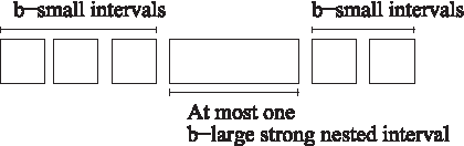
The structure of b-nested common intervals given by consecutive children of a Q-node is more complex. In the next lemmas we show that at most one of the intervals Int(xi) composing such an interval may be b-large (see also Fig. 2).
The structure of a b-nested Q-interval.
Lemma 3
Let I be a Q-interval with\documentclass{aastex}\usepackage{amsbsy}\usepackage{amsfonts}\usepackage{amssymb}\usepackage{bm}\usepackage{mathrsfs}\usepackage{pifont}\usepackage{stmaryrd}\usepackage{textcomp}\usepackage{portland, xspace}\usepackage{amsmath, amsxtra}\pagestyle{empty}\DeclareMathSizes{10}{9}{7}{6}\begin{document}
$$D ( I ) = \{x_1 , x_2 , \ldots , x_r \} $$
\end{document}. Then I is a b-nested common interval if and only if Int(x1) is b-small and I − Int(x1) is a b-nested common interval, or Int(xr) is b-small and I − Int(xr) is a b-nested common interval.
Proof. Recall that for a Q-interval I, the order \documentclass{aastex}\usepackage{amsbsy}\usepackage{amsfonts}\usepackage{amssymb}\usepackage{bm}\usepackage{mathrsfs}\usepackage{pifont}\usepackage{stmaryrd}\usepackage{textcomp}\usepackage{portland, xspace}\usepackage{amsmath, amsxtra}\pagestyle{empty}\DeclareMathSizes{10}{9}{7}{6}\begin{document}
$$x_1 , x_2 , \ldots , x_r$$
\end{document} implies that the equation max(Int(xi)) + 1 = min(Int(xi+1)) holds for all i with 1 ≤ i < r.
⇒ : Since I is b-nested, it contains some b-nested interval J such that |I| > |J| ≥ |I|−b. Choose J as large as possible. Now, J cannot be strictly included in some non–b-nested Int(xi) by Remark 2, thus \documentclass{aastex}\usepackage{amsbsy}\usepackage{amsfonts}\usepackage{amssymb}\usepackage{bm}\usepackage{mathrsfs}\usepackage{pifont}\usepackage{stmaryrd}\usepackage{textcomp}\usepackage{portland, xspace}\usepackage{amsmath, amsxtra}\pagestyle{empty}\DeclareMathSizes{10}{9}{7}{6}\begin{document}
$$D ( J ) = \{x_p , x_{p + 1} , \ldots , x_s \} $$
\end{document} with p ≥ 1,s ≤ r, and p ≠ 1 or s ≠ r. Assume w.l.o.g. that p > 1. Then Int(x1) is b-small (since |J| ≥ |I|−b), and I −Int(x1) is b-nested by Remark 2 since it contains J or is equal to J.
⇐ : Let j = 1 or j = r according to which proposition holds. We have that |I − Int(xj)| = |I|−|Int(xj)| ≥ |I|−b since |Int(xj)| ≤ b. Then I is b-nested. ■
Lemma 4
Let I be a Q-interval with\documentclass{aastex}\usepackage{amsbsy}\usepackage{amsfonts}\usepackage{amssymb}\usepackage{bm}\usepackage{mathrsfs}\usepackage{pifont}\usepackage{stmaryrd}\usepackage{textcomp}\usepackage{portland, xspace}\usepackage{amsmath, amsxtra}\pagestyle{empty}\DeclareMathSizes{10}{9}{7}{6}\begin{document}
$$D ( I ) = \{x_1 , x_2 , \ldots , x_r \} $$
\end{document}, which is a b-nested common interval. Then at most one of the intervals Int(xi), 1 ≤ i ≤ r, is b-large, and in this case, this interval is a b-nested common interval.
Proof. By contradiction, assume there exist b-nested common Q-intervals that contain at least two b-large intervals of type Int(xi), and let I be a smallest such interval w.r.t. inclusion. Let xu (resp. xv), with 1 ≤ u,v ≤ r, be such that Int(xu) (resp. Int(xv)) is b-large and u (resp. v) is minimum (resp. maximum) with this property. Then u = 1 and v = r, otherwise by Lemma 3 the minimality of I is contradicted. But now Lemma 3 is contradicted, since Int(x1) and Int(xr) are both b-large.
Then, at most one of the intervals Int(xi), 1 ≤ i ≤ r, is b-large. To finish the proof, assume that Int(xi) (for some fixed i), is the unique b-large interval and apply Lemma 1 to Int(xi) to deduce that Int(xi) is b-nested. ■
We are able now to prove the theorem characterizing b-nested common intervals.
Theorem 3
Let I be a common interval of\documentclass{aastex}\usepackage{amsbsy}\usepackage{amsfonts}\usepackage{amssymb}\usepackage{bm}\usepackage{mathrsfs}\usepackage{pifont}\usepackage{stmaryrd}\usepackage{textcomp}\usepackage{portland, xspace}\usepackage{amsmath, amsxtra}\pagestyle{empty}\DeclareMathSizes{10}{9}{7}{6}\begin{document}
$${\cal P}$$
\end{document}. I is b-nested if and only if:
(a) Either I is a P-interval and there exists\documentclass{aastex}\usepackage{amsbsy}\usepackage{amsfonts}\usepackage{amssymb}\usepackage{bm}\usepackage{mathrsfs}\usepackage{pifont}\usepackage{stmaryrd}\usepackage{textcomp}\usepackage{portland, xspace}\usepackage{amsmath, amsxtra}\pagestyle{empty}\DeclareMathSizes{10}{9}{7}{6}\begin{document}
$$x_h \in D ( I )$$
\end{document}such that Int(xh) is a b-nested common interval of size at least |I|−b.
(b) or I is a Q-interval with the property that all intervals Int(xi) with\documentclass{aastex}\usepackage{amsbsy}\usepackage{amsfonts}\usepackage{amssymb}\usepackage{bm}\usepackage{mathrsfs}\usepackage{pifont}\usepackage{stmaryrd}\usepackage{textcomp}\usepackage{portland, xspace}\usepackage{amsmath, amsxtra}\pagestyle{empty}\DeclareMathSizes{10}{9}{7}{6}\begin{document}
$$x_i \in D ( I )$$
\end{document}are b-small, with one possible exception, which is a b-large b-nested interval.
Proof.Lemma 2 proves the theorem in the case where I is a P-interval. When I is a Q-interval, Lemma 4 proves affirmation (b). ■
3.3. Computing and counting all b-nested common intervals
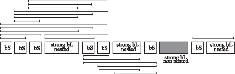
Consider Algorithm 1, which computes all b-nested common intervals. For a node xc, the notations min(c) and max(c) respectively indicate the minimum and the maximum value in Int(xc). Figure 3 illustrates our algorithm.
Computing all b-nested intervals of a Q-interval, where bS (resp. bL) means b-small (resp. b-large). The algorithm considers all positions from left to right and expands the b-nested interval when possible.
Input: The PQ-tree T = (V, E) of \documentclass{aastex}\usepackage{amsbsy}\usepackage{amsfonts}\usepackage{amssymb}\usepackage{bm}\usepackage{mathrsfs}\usepackage{pifont}\usepackage{stmaryrd}\usepackage{textcomp}\usepackage{portland, xspace}\usepackage{amsmath, amsxtra}\pagestyle{empty}\DeclareMathSizes{10}{9}{7}{6}\begin{document}
$${\cal P}$$
\end{document} for common intervals, a positive integer b
Output: All b-nested common intervals of \documentclass{aastex}\usepackage{amsbsy}\usepackage{amsfonts}\usepackage{amssymb}\usepackage{bm}\usepackage{mathrsfs}\usepackage{pifont}\usepackage{stmaryrd}\usepackage{textcomp}\usepackage{portland, xspace}\usepackage{amsmath, amsxtra}\pagestyle{empty}\DeclareMathSizes{10}{9}{7}{6}\begin{document}
$${\cal P}$$
\end{document}
The b-NestedCommonSearch algorithm
1
Perform a post-order traversal of T;
2
foreach node x of T encountered during this traversaldo
3
if x is a leafthen
4
output Int(x) as b-nested;
5
else
6
let \documentclass{aastex}\usepackage{amsbsy}\usepackage{amsfonts}\usepackage{amssymb}\usepackage{bm}\usepackage{mathrsfs}\usepackage{pifont}\usepackage{stmaryrd}\usepackage{textcomp}\usepackage{portland, xspace}\usepackage{amsmath, amsxtra}\pagestyle{empty}\DeclareMathSizes{10}{9}{7}{6}\begin{document}
$$x_1 , x_2 \ldots , x_p$$
\end{document} be the children of x ;
7
ifx is a P-nodethen
8
if ∃ i such that Int(xi) is b-nested and |Int(xi)| ≥ |Int(x)|− b
then
9
output Int(x) as b-nested
10
end if
11
else
12
forc ← 1 to pdo
13
large ← 0 // number of b-large intervals already included;
14
d ← c // considers all children starting with xc;
15
whiled ≤ p and (|Int(xd)| ≤ b or Int(xd) is b-nested) and large ≤ 1 do
16
if |Int(xd)| > bthenlarge ← large + 1endif;
17
ifc < d and large ≤ 1 then
18
output (min(c).max(d)) as b-nested;
19
end if
20
d ← d + 1;
21
end while
22
end for
23
end if
24
end if
25
end for
Theorem 4
Algorithm 1 correctly computes all the b-nested common intervals, assuming the PQ-tree is already built, in O(n + nocc) time, where nocc is the number of b-nested common intervals in\documentclass{aastex}\usepackage{amsbsy}\usepackage{amsfonts}\usepackage{amssymb}\usepackage{bm}\usepackage{mathrsfs}\usepackage{pifont}\usepackage{stmaryrd}\usepackage{textcomp}\usepackage{portland, xspace}\usepackage{amsmath, amsxtra}\pagestyle{empty}\DeclareMathSizes{10}{9}{7}{6}\begin{document}
$${\cal P}$$
\end{document}.
Proof. To show the algorithm correctness, note first that all the leaves are output in step 4, and they are b-nested common intervals. Moreover, all b-nested common intervals corresponding to P-nodes are correctly output in step 9 according to Theorem 3(a). Next, Q-intervals corresponding to a Q-node x are generated in steps 12–22 by starting with each child xc of x, and successively adding right children xd as long as condition (b) in Theorem 3 is satisfied (step 15).
Let us analyze now the running time. The PQ-tree has size O(n), and the traversal considers every node x exactly once. Working once on the children of each node takes O(n). The test in line 8 considers every child of a P-node one more time, so that the O(n) time is ensured when the Q-interval generation is left apart. Now, during the generation of the Q-intervals, a node xd that belongs to no b-nested common interval is uselessly included in some interval candidate at most once by left initial positions for the scan (beginning line 12), which is in total bounded by n since there exists a linear number of initial positions in the PQ-tree. At each iteration of the loop line 15, a unique distinct b-nested interval is output, or c = d (which happens once for each node since d is incremented at each iteration), or large = 2 (which also happens once for each node since it ends the loop). The total number of iterations is thus O(n + nocc), each iteration taking O(1). The overall running time is thus in O(n + nocc), where nocc is the total number of b-nested common intervals. ■
The previous approach can be modified to count the b-nested common intervals instead of enumerating them by simply analyzing more precisely the structure of the Q-nodes. The goal is to count the b-nested common intervals in a time proportional to the number of children instead of the number of b-nested common intervals. To perform the count, we assume that the traversal is post-order, that it marks each vertex as b-nested or not, and that it computes the cardinality of each Int(xi).
P-nodes. Obviously, a P-node (including the leaves) counts for 1 if the associated interval is b-nested, and for 0 otherwise.
Q-nodes. To make the computation for a Q-node with children \documentclass{aastex}\usepackage{amsbsy}\usepackage{amsfonts}\usepackage{amssymb}\usepackage{bm}\usepackage{mathrsfs}\usepackage{pifont}\usepackage{stmaryrd}\usepackage{textcomp}\usepackage{portland, xspace}\usepackage{amsmath, amsxtra}\pagestyle{empty}\DeclareMathSizes{10}{9}{7}{6}\begin{document}
$$\{x_1 , x_2 , \ldots , x_p \} $$
\end{document}, the algorithm looks for the b-large b-nested intervals Int(xd) and counts (1) the b-nested common intervals containing each Int(xd), and (2) the b-nested common intervals generated by maximal sets of consecutive b-small common intervals Int(xi). To this end, the vertices xi are considered from left to right in order to identify both the b-large b-nested common intervals Int(xd), and the maximal sets of consecutive b-small common intervals Int(xi). Then:
To solve (1), each encountered b-large b-nested interval Int(xd) has the following treatment. We count the number of consecutive b-small nodes xi on its right (resp. left), denoted by r(d) [resp. l(d)]. Then we compute the number of b-nested common intervals that contain child xd as
\documentclass{aastex}\usepackage{amsbsy}\usepackage{amsfonts}\usepackage{amssymb}\usepackage{bm}\usepackage{mathrsfs}\usepackage{pifont}\usepackage{stmaryrd}\usepackage{textcomp}\usepackage{portland, xspace}\usepackage{amsmath, amsxtra}\pagestyle{empty}\DeclareMathSizes{10}{9}{7}{6}\begin{document}
\begin{align*}l ( d ) * ( r ( d ) + 1 ) + r ( d ) .\end{align*}
\end{document}
To solve (2), for each maximal set of consecutive b-small common intervals Int(xi), assuming it has size h, we count
\documentclass{aastex}\usepackage{amsbsy}\usepackage{amsfonts}\usepackage{amssymb}\usepackage{bm}\usepackage{mathrsfs}\usepackage{pifont}\usepackage{stmaryrd}\usepackage{textcomp}\usepackage{portland, xspace}\usepackage{amsmath, amsxtra}\pagestyle{empty}\DeclareMathSizes{10}{9}{7}{6}\begin{document}
\begin{align*}h* ( h - 1 ) / 2.\end{align*}
\end{document}
One may easily decide whether the interval corresponding to the Q-node itself is b-nested or not and compute its size.
All these operations may be performed in O(k) time, where k is the number of sons of the Q-node.
Example. In the Figure 3 example, we count (from left to right): (a) for the first b-large strong child to the left: 3 * (2 + 1) + 2 = 11 b-nested common intervals; (b) for the b-large second strong child: 2 * (1 + 1) + 1 = 5 b-nested common intervals; and (c) for the last b-large strong child: 1 * (0 + 1) = 1 b-nested common intervals. We sum up to obtain 17 b-nested common intervals containing one b-large b-nested interval Int(xi). Now we add the nested intervals generated between the b-large intervals: 3 + 1 = 4. Altogether, the Q-node of Figure 3 generates 21 b-nested intervals.
Complexity. The time complexity of the counting procedure is obviously O(n), the size of the underlying PQ-tree. The time needed to get the PQ-tree itself given K permutations is however O(Kn), as indicated before.
4. On b-nested Conserved Intervals
As stated before, we assume the set \documentclass{aastex}\usepackage{amsbsy}\usepackage{amsfonts}\usepackage{amssymb}\usepackage{bm}\usepackage{mathrsfs}\usepackage{pifont}\usepackage{stmaryrd}\usepackage{textcomp}\usepackage{portland, xspace}\usepackage{amsmath, amsxtra}\pagestyle{empty}\DeclareMathSizes{10}{9}{7}{6}\begin{document}
$${\cal P}$$
\end{document} of permutations has the properties required in Definition 2. As conserved intervals are common intervals, one may be tempted to follow the same approach using PQ-trees. Unfortunately, the inclusion tree of strong conserved intervals does not define a PQ-tree representing the family of conserved intervals because a conserved interval cannot be written as a disjoint union of strong conserved intervals. The resulting ordered tree has been used in the literature (Bergeron et al., 2004), but its underlying properties have not been clearly stated. We do it here before using these properties.
4.1. Structure of conserved intervals
We start with an easy property about intersection of conserved intervals:
Lemma 5
Let I = (u.v) and J = (c.d) be two conserved intervals of\documentclass{aastex}\usepackage{amsbsy}\usepackage{amsfonts}\usepackage{amssymb}\usepackage{bm}\usepackage{mathrsfs}\usepackage{pifont}\usepackage{stmaryrd}\usepackage{textcomp}\usepackage{portland, xspace}\usepackage{amsmath, amsxtra}\pagestyle{empty}\DeclareMathSizes{10}{9}{7}{6}\begin{document}
$${\cal P}$$
\end{document}with u < c ≤ v < d. Then the intervals (u.c), (c.v), (v.d), and (u.d) are conserved intervals.
Proof. As an element x from I fulfills u ≤ x ≤ v, and an element y from J fulfills c ≤ y ≤ d then an element z from I\J fulfills u ≤ z < c. These elements are exactly those between u and c, and (u.c) is thus a conserved interval. Similarly, J\I = (v.d). The elements from I ∩ J are all the elements not lower than v and not larger than c, so (c.v) is a conserved interval. Finally, the elements from I ∪ J are all elements greater than u and smaller than d, so (u.d) is a conserved interval. ■
The notions of strong/weak intervals and of a frontier are essential in our study.
Definition 8
A conserved interval I of\documentclass{aastex}\usepackage{amsbsy}\usepackage{amsfonts}\usepackage{amssymb}\usepackage{bm}\usepackage{mathrsfs}\usepackage{pifont}\usepackage{stmaryrd}\usepackage{textcomp}\usepackage{portland, xspace}\usepackage{amsmath, amsxtra}\pagestyle{empty}\DeclareMathSizes{10}{9}{7}{6}\begin{document}
$${\cal P}$$
\end{document}is strong if it has cardinality at least two and does not overlap other conserved intervals. Otherwise, it is weak.
Notice that unit conserved intervals are not strong.
Definition 9
Let I = (a.c) be a conserved interval. A set\documentclass{aastex}\usepackage{amsbsy}\usepackage{amsfonts}\usepackage{amssymb}\usepackage{bm}\usepackage{mathrsfs}\usepackage{pifont}\usepackage{stmaryrd}\usepackage{textcomp}\usepackage{portland, xspace}\usepackage{amsmath, amsxtra}\pagestyle{empty}\DeclareMathSizes{10}{9}{7}{6}\begin{document}
$$\{f_1 , \ldots , f_k \} $$
\end{document}of elements satisfying\documentclass{aastex}\usepackage{amsbsy}\usepackage{amsfonts}\usepackage{amssymb}\usepackage{bm}\usepackage{mathrsfs}\usepackage{pifont}\usepackage{stmaryrd}\usepackage{textcomp}\usepackage{portland, xspace}\usepackage{amsmath, amsxtra}\pagestyle{empty}\DeclareMathSizes{10}{9}{7}{6}\begin{document}
$$a = f_1 < f_2 < \ldots < f_k = c$$
\end{document}is a set of frontiers of I if (fi.fj) is a conserved interval, for all i,j with 1 ≤ i < j ≤ k. An element of I is a frontier of I if it occurs in at least one set of frontiers of I.
The two following properties are easy ones:
Lemma 6
Let I = (a.c) be a conserved interval and F be a set of frontiers of I. The elements of F are either all positive or all negative.
Proof. By the definition of a conserved interval, its two endpoints have the same sign. By the definition of a set of frontiers, any two frontiers are the extremities of some conserved interval.
Lemma 7
Let I = (a.c) be a conserved interval, and let\documentclass{aastex}\usepackage{amsbsy}\usepackage{amsfonts}\usepackage{amssymb}\usepackage{bm}\usepackage{mathrsfs}\usepackage{pifont}\usepackage{stmaryrd}\usepackage{textcomp}\usepackage{portland, xspace}\usepackage{amsmath, amsxtra}\pagestyle{empty}\DeclareMathSizes{10}{9}{7}{6}\begin{document}
$$F = \{f_1 , \ldots , f_k \} $$
\end{document}and\documentclass{aastex}\usepackage{amsbsy}\usepackage{amsfonts}\usepackage{amssymb}\usepackage{bm}\usepackage{mathrsfs}\usepackage{pifont}\usepackage{stmaryrd}\usepackage{textcomp}\usepackage{portland, xspace}\usepackage{amsmath, amsxtra}\pagestyle{empty}\DeclareMathSizes{10}{9}{7}{6}\begin{document}
$$F^{\prime} = \{f^{\prime}_1 , \ldots , f^{\prime}_l \} $$
\end{document}be two sets of frontiers of I. Then F ∪ F′ is also a set of frontiers of I.
Proof. We show that any interval between two elements of F ∪ F′ is conserved. Let \documentclass{aastex}\usepackage{amsbsy}\usepackage{amsfonts}\usepackage{amssymb}\usepackage{bm}\usepackage{mathrsfs}\usepackage{pifont}\usepackage{stmaryrd}\usepackage{textcomp}\usepackage{portland, xspace}\usepackage{amsmath, amsxtra}\pagestyle{empty}\DeclareMathSizes{10}{9}{7}{6}\begin{document}
$$f_i \in F$$
\end{document} and \documentclass{aastex}\usepackage{amsbsy}\usepackage{amsfonts}\usepackage{amssymb}\usepackage{bm}\usepackage{mathrsfs}\usepackage{pifont}\usepackage{stmaryrd}\usepackage{textcomp}\usepackage{portland, xspace}\usepackage{amsmath, amsxtra}\pagestyle{empty}\DeclareMathSizes{10}{9}{7}{6}\begin{document}
$$f^{\prime}_j \in F^{\prime}$$
\end{document}, and suppose that \documentclass{aastex}\usepackage{amsbsy}\usepackage{amsfonts}\usepackage{amssymb}\usepackage{bm}\usepackage{mathrsfs}\usepackage{pifont}\usepackage{stmaryrd}\usepackage{textcomp}\usepackage{portland, xspace}\usepackage{amsmath, amsxtra}\pagestyle{empty}\DeclareMathSizes{10}{9}{7}{6}\begin{document}
$$f_i < f_j^{\prime}$$
\end{document}. If fi = a, then we have \documentclass{aastex}\usepackage{amsbsy}\usepackage{amsfonts}\usepackage{amssymb}\usepackage{bm}\usepackage{mathrsfs}\usepackage{pifont}\usepackage{stmaryrd}\usepackage{textcomp}\usepackage{portland, xspace}\usepackage{amsmath, amsxtra}\pagestyle{empty}\DeclareMathSizes{10}{9}{7}{6}\begin{document}
$$( f_i.f_j^{\prime} ) = ( f_1^{\prime}.f_j^{\prime} )$$
\end{document} and we are done. If \documentclass{aastex}\usepackage{amsbsy}\usepackage{amsfonts}\usepackage{amssymb}\usepackage{bm}\usepackage{mathrsfs}\usepackage{pifont}\usepackage{stmaryrd}\usepackage{textcomp}\usepackage{portland, xspace}\usepackage{amsmath, amsxtra}\pagestyle{empty}\DeclareMathSizes{10}{9}{7}{6}\begin{document}
$$f_j^{\prime} = c$$
\end{document}, then \documentclass{aastex}\usepackage{amsbsy}\usepackage{amsfonts}\usepackage{amssymb}\usepackage{bm}\usepackage{mathrsfs}\usepackage{pifont}\usepackage{stmaryrd}\usepackage{textcomp}\usepackage{portland, xspace}\usepackage{amsmath, amsxtra}\pagestyle{empty}\DeclareMathSizes{10}{9}{7}{6}\begin{document}
$$( f_i.f_j^{\prime} ) = ( f_i.f_k )$$
\end{document} and we are also done. If fi ≠ a and \documentclass{aastex}\usepackage{amsbsy}\usepackage{amsfonts}\usepackage{amssymb}\usepackage{bm}\usepackage{mathrsfs}\usepackage{pifont}\usepackage{stmaryrd}\usepackage{textcomp}\usepackage{portland, xspace}\usepackage{amsmath, amsxtra}\pagestyle{empty}\DeclareMathSizes{10}{9}{7}{6}\begin{document}
$$f_j^{\prime} \ne c$$
\end{document}, then Lemma 5 concludes. The same proof holds if \documentclass{aastex}\usepackage{amsbsy}\usepackage{amsfonts}\usepackage{amssymb}\usepackage{bm}\usepackage{mathrsfs}\usepackage{pifont}\usepackage{stmaryrd}\usepackage{textcomp}\usepackage{portland, xspace}\usepackage{amsmath, amsxtra}\pagestyle{empty}\DeclareMathSizes{10}{9}{7}{6}\begin{document}
$$f_i > f_j^{\prime}$$
\end{document}. ■
Now let T be the inclusion tree of strong intervals from \documentclass{aastex}\usepackage{amsbsy}\usepackage{amsfonts}\usepackage{amssymb}\usepackage{bm}\usepackage{mathrsfs}\usepackage{pifont}\usepackage{stmaryrd}\usepackage{textcomp}\usepackage{portland, xspace}\usepackage{amsmath, amsxtra}\pagestyle{empty}\DeclareMathSizes{10}{9}{7}{6}\begin{document}
$${\cal P}$$
\end{document}, in which every node x corresponds to a strong interval denoted Int(x), and node x is the parent of node y iff Int(x) is the smallest strong conserved interval strictly containing Int(y). Then T contains two types of nodes: those corresponding to strong conserved intervals with no internal frontier and those corresponding to strong conserved intervals with at least one internal frontier. We will show that weak conserved intervals are the conserved strict subintervals of the latter ones, defined by two frontiers. Overall, we have a structure working pretty much as a PQ-tree, but which cannot be mapped to a PQ-tree. This is proved in the next theorem.
Given a conserved interval, denote by Container(I) the smallest strong conserved interval such that I ⊆ J.
Theorem 5
Each conserved interval I of\documentclass{aastex}\usepackage{amsbsy}\usepackage{amsfonts}\usepackage{amssymb}\usepackage{bm}\usepackage{mathrsfs}\usepackage{pifont}\usepackage{stmaryrd}\usepackage{textcomp}\usepackage{portland, xspace}\usepackage{amsmath, amsxtra}\pagestyle{empty}\DeclareMathSizes{10}{9}{7}{6}\begin{document}
$${\cal P}$$
\end{document}admits a unique maximal (w.r.t. inclusion) set of frontiers denoted FI. Moreover, each conserved interval I of\documentclass{aastex}\usepackage{amsbsy}\usepackage{amsfonts}\usepackage{amssymb}\usepackage{bm}\usepackage{mathrsfs}\usepackage{pifont}\usepackage{stmaryrd}\usepackage{textcomp}\usepackage{portland, xspace}\usepackage{amsmath, amsxtra}\pagestyle{empty}\DeclareMathSizes{10}{9}{7}{6}\begin{document}
$${\cal P}$$
\end{document}satisfies one of the following properties:
1.I is strong.
2.I is weak and there exists a unique strong conserved interval J of\documentclass{aastex}\usepackage{amsbsy}\usepackage{amsfonts}\usepackage{amssymb}\usepackage{bm}\usepackage{mathrsfs}\usepackage{pifont}\usepackage{stmaryrd}\usepackage{textcomp}\usepackage{portland, xspace}\usepackage{amsmath, amsxtra}\pagestyle{empty}\DeclareMathSizes{10}{9}{7}{6}\begin{document}
$${\cal P}$$
\end{document}, and two frontiers\documentclass{aastex}\usepackage{amsbsy}\usepackage{amsfonts}\usepackage{amssymb}\usepackage{bm}\usepackage{mathrsfs}\usepackage{pifont}\usepackage{stmaryrd}\usepackage{textcomp}\usepackage{portland, xspace}\usepackage{amsmath, amsxtra}\pagestyle{empty}\DeclareMathSizes{10}{9}{7}{6}\begin{document}
$$f_i , f_j \in F_J$$
\end{document}, with fi < fj, such that I = (fi.fj). Moreover, FI = FJ ∩ I and J = Container(I).
Proof. Let us first prove the uniqueness of the maximal set of frontiers. By contradiction, assume two distinct maximal sets of frontiers \documentclass{aastex}\usepackage{amsbsy}\usepackage{amsfonts}\usepackage{amssymb}\usepackage{bm}\usepackage{mathrsfs}\usepackage{pifont}\usepackage{stmaryrd}\usepackage{textcomp}\usepackage{portland, xspace}\usepackage{amsmath, amsxtra}\pagestyle{empty}\DeclareMathSizes{10}{9}{7}{6}\begin{document}
$$F = \{f_1 , \ldots , f_k \} $$
\end{document} and \documentclass{aastex}\usepackage{amsbsy}\usepackage{amsfonts}\usepackage{amssymb}\usepackage{bm}\usepackage{mathrsfs}\usepackage{pifont}\usepackage{stmaryrd}\usepackage{textcomp}\usepackage{portland, xspace}\usepackage{amsmath, amsxtra}\pagestyle{empty}\DeclareMathSizes{10}{9}{7}{6}\begin{document}
$$F^{\prime} = \{f_1^{\prime} , \ldots , f_l^{\prime} \} $$
\end{document} exist for a conserved interval I. Using Lemma 7, we deduce that F ∪ F′ is a larger set of frontiers of I, a contradiction.
Let us now prove that if I is not strong, then there exists a unique strong conserved interval J, and two frontiers \documentclass{aastex}\usepackage{amsbsy}\usepackage{amsfonts}\usepackage{amssymb}\usepackage{bm}\usepackage{mathrsfs}\usepackage{pifont}\usepackage{stmaryrd}\usepackage{textcomp}\usepackage{portland, xspace}\usepackage{amsmath, amsxtra}\pagestyle{empty}\DeclareMathSizes{10}{9}{7}{6}\begin{document}
$$f_i , f_j \in F_J$$
\end{document} with fi < fj, such that I = (fi.fj).
Existence of J. Let I1 = I = (a0.a1) be a weak conserved interval of \documentclass{aastex}\usepackage{amsbsy}\usepackage{amsfonts}\usepackage{amssymb}\usepackage{bm}\usepackage{mathrsfs}\usepackage{pifont}\usepackage{stmaryrd}\usepackage{textcomp}\usepackage{portland, xspace}\usepackage{amsmath, amsxtra}\pagestyle{empty}\DeclareMathSizes{10}{9}{7}{6}\begin{document}
$${\cal P}$$
\end{document}. Then there is another interval I2 overlapping it, either on its left [i.e., I2 = (a2.x2) with a2 < a0 ≤ x2 < a1] or on its right [i.e., I2 = (x2.a2) with a0 < x2 ≤ a1 < a2]. According to Lemma 5, J2 = I1 ∪ I2 is a conserved interval, and F2 = {a0, a1, a2, x2} is a set of frontiers for J2 (not necessarily all distinct). If J2 is not strong then it is overlapped by another interval I3. We build an increasing sequence of intervals \documentclass{aastex}\usepackage{amsbsy}\usepackage{amsfonts}\usepackage{amssymb}\usepackage{bm}\usepackage{mathrsfs}\usepackage{pifont}\usepackage{stmaryrd}\usepackage{textcomp}\usepackage{portland, xspace}\usepackage{amsmath, amsxtra}\pagestyle{empty}\DeclareMathSizes{10}{9}{7}{6}\begin{document}
$$J_1 = I_1 , J_2 , \ldots , J_k$$
\end{document}, with Ji overlapped by Ii+1, and Ji+1 = Ji ∪ Ii+1, until we find a strong conserved interval Jk [the process ends since (1.n) is strong]. Each time Lemma 5 ensures that Ji+1 is a conserved interval, and Fi+1 = Fi ∪ {ai+1, xi+1} is a set of frontiers for Ji+1 (where ai+1, xi+1 are the endpoins of Ii+1). But then Fk is a subset of the maximal set of frontiers FJk of Jk, and the two frontiers of Jk defining I1 are a0, a1, since \documentclass{aastex}\usepackage{amsbsy}\usepackage{amsfonts}\usepackage{amssymb}\usepackage{bm}\usepackage{mathrsfs}\usepackage{pifont}\usepackage{stmaryrd}\usepackage{textcomp}\usepackage{portland, xspace}\usepackage{amsmath, amsxtra}\pagestyle{empty}\DeclareMathSizes{10}{9}{7}{6}\begin{document}
$$\{a_0 , a_1 \} \subseteq F_2 \subseteq F_3 \subseteq \ldots \subseteq F_k \subseteq F_{J_k}$$
\end{document}.
Uniqueness of J. Assume a contrario that two strong intervals J1 and J2 exist with \documentclass{aastex}\usepackage{amsbsy}\usepackage{amsfonts}\usepackage{amssymb}\usepackage{bm}\usepackage{mathrsfs}\usepackage{pifont}\usepackage{stmaryrd}\usepackage{textcomp}\usepackage{portland, xspace}\usepackage{amsmath, amsxtra}\pagestyle{empty}\DeclareMathSizes{10}{9}{7}{6}\begin{document}
$$F_{J_1} = \{f_1 , \ldots , f_p \} , F_{J_2} = \{f_1^{\prime} , \ldots , f_r^{\prime} \} $$
\end{document} and such that \documentclass{aastex}\usepackage{amsbsy}\usepackage{amsfonts}\usepackage{amssymb}\usepackage{bm}\usepackage{mathrsfs}\usepackage{pifont}\usepackage{stmaryrd}\usepackage{textcomp}\usepackage{portland, xspace}\usepackage{amsmath, amsxtra}\pagestyle{empty}\DeclareMathSizes{10}{9}{7}{6}\begin{document}
$$I = ( f_i.f_j ) = ( f_k^{\prime}.f_l^{\prime} )$$
\end{document} with 1 ≤ i < j ≤ p and 1 ≤ k < l ≤ r. Then, clearly, \documentclass{aastex}\usepackage{amsbsy}\usepackage{amsfonts}\usepackage{amssymb}\usepackage{bm}\usepackage{mathrsfs}\usepackage{pifont}\usepackage{stmaryrd}\usepackage{textcomp}\usepackage{portland, xspace}\usepackage{amsmath, amsxtra}\pagestyle{empty}\DeclareMathSizes{10}{9}{7}{6}\begin{document}
$$f_i = f_k^{\prime}$$
\end{document} and this is the left endpoint of I, whereas \documentclass{aastex}\usepackage{amsbsy}\usepackage{amsfonts}\usepackage{amssymb}\usepackage{bm}\usepackage{mathrsfs}\usepackage{pifont}\usepackage{stmaryrd}\usepackage{textcomp}\usepackage{portland, xspace}\usepackage{amsmath, amsxtra}\pagestyle{empty}\DeclareMathSizes{10}{9}{7}{6}\begin{document}
$$f_j = f_l^{\prime}$$
\end{document} and this is the right endpoint of I. Since J1 and J2 are both strong, they cannot overlap. Assume then w.l.o.g. that J1 is strictly included in J2, and more precisely that \documentclass{aastex}\usepackage{amsbsy}\usepackage{amsfonts}\usepackage{amssymb}\usepackage{bm}\usepackage{mathrsfs}\usepackage{pifont}\usepackage{stmaryrd}\usepackage{textcomp}\usepackage{portland, xspace}\usepackage{amsmath, amsxtra}\pagestyle{empty}\DeclareMathSizes{10}{9}{7}{6}\begin{document}
$$f_p \neq f_r^{\prime}$$
\end{document} (then \documentclass{aastex}\usepackage{amsbsy}\usepackage{amsfonts}\usepackage{amssymb}\usepackage{bm}\usepackage{mathrsfs}\usepackage{pifont}\usepackage{stmaryrd}\usepackage{textcomp}\usepackage{portland, xspace}\usepackage{amsmath, amsxtra}\pagestyle{empty}\DeclareMathSizes{10}{9}{7}{6}\begin{document}
$$f_p < f_r^{\prime}$$
\end{document} due to inclusion). Now, (\documentclass{aastex}\usepackage{amsbsy}\usepackage{amsfonts}\usepackage{amssymb}\usepackage{bm}\usepackage{mathrsfs}\usepackage{pifont}\usepackage{stmaryrd}\usepackage{textcomp}\usepackage{portland, xspace}\usepackage{amsmath, amsxtra}\pagestyle{empty}\DeclareMathSizes{10}{9}{7}{6}\begin{document}
$$f_k^{\prime}.f_r^{\prime}$$
\end{document}) overlaps J1 (which is forbidden) unless i = 1, in which case we have \documentclass{aastex}\usepackage{amsbsy}\usepackage{amsfonts}\usepackage{amssymb}\usepackage{bm}\usepackage{mathrsfs}\usepackage{pifont}\usepackage{stmaryrd}\usepackage{textcomp}\usepackage{portland, xspace}\usepackage{amsmath, amsxtra}\pagestyle{empty}\DeclareMathSizes{10}{9}{7}{6}\begin{document}
$$f_1 = f_i = f_k^{\prime}$$
\end{document}, and this is the left endpoint of I. Now, since I is strictly included in J, we deduce j < p and (\documentclass{aastex}\usepackage{amsbsy}\usepackage{amsfonts}\usepackage{amssymb}\usepackage{bm}\usepackage{mathrsfs}\usepackage{pifont}\usepackage{stmaryrd}\usepackage{textcomp}\usepackage{portland, xspace}\usepackage{amsmath, amsxtra}\pagestyle{empty}\DeclareMathSizes{10}{9}{7}{6}\begin{document}
$$f_l^{\prime}.f_r^{\prime}$$
\end{document}) overlaps J1. This contradiction proves the uniqueness of the strong interval J satisfying condition 2.
Let us prove that FI = FJ ∩ I. Suppose by contradiction that FI contains a frontier f not in FJ. Recall that I = (a0.a1) and a0, a1 belong to FJ. Now, for each \documentclass{aastex}\usepackage{amsbsy}\usepackage{amsfonts}\usepackage{amssymb}\usepackage{bm}\usepackage{mathrsfs}\usepackage{pifont}\usepackage{stmaryrd}\usepackage{textcomp}\usepackage{portland, xspace}\usepackage{amsmath, amsxtra}\pagestyle{empty}\DeclareMathSizes{10}{9}{7}{6}\begin{document}
$$f_l \in F_J$$
\end{document} with fl < f, we have that (fl.f) is a conserved interval either by Lemma 5 applied to (a0.f) and (f1.fl) (when fl ≥ a0), or since it is the union of the two conserved intervals (fl.a0) and (a.f) (when fl < a0). Symmetrically, (f.fl) is also a conserved interval when \documentclass{aastex}\usepackage{amsbsy}\usepackage{amsfonts}\usepackage{amssymb}\usepackage{bm}\usepackage{mathrsfs}\usepackage{pifont}\usepackage{stmaryrd}\usepackage{textcomp}\usepackage{portland, xspace}\usepackage{amsmath, amsxtra}\pagestyle{empty}\DeclareMathSizes{10}{9}{7}{6}\begin{document}
$$f_l \in F_J$$
\end{document}, fl > f. But then FJ ∪ {f} is a set of frontiers of J larger than FJ, which contradicts the maximality of FJ.
Eventually, let us prove that J = Container(I). Assume that \documentclass{aastex}\usepackage{amsbsy}\usepackage{amsfonts}\usepackage{amssymb}\usepackage{bm}\usepackage{mathrsfs}\usepackage{pifont}\usepackage{stmaryrd}\usepackage{textcomp}\usepackage{portland, xspace}\usepackage{amsmath, amsxtra}\pagestyle{empty}\DeclareMathSizes{10}{9}{7}{6}\begin{document}
$$F = \{f_1 , f_2 , \ldots , f_k \} $$
\end{document}, that I = (fi.fj), and that, by contradiction, there is a smallest strong conserved interval J′ = (a.c) that contains I. Then J′ ⊊ J since otherwise J and J′ would overlap. W.l.o.g. assume that fj ≠ c. Then (fi.fk) overlaps J′, and this contradicts the assumption that J′ is strong. ■
We only need three more results before dealing with b-nested conserved intervals.
Lemma 8
Let I and J be two conserved intervals. If there exists a frontier\documentclass{aastex}\usepackage{amsbsy}\usepackage{amsfonts}\usepackage{amssymb}\usepackage{bm}\usepackage{mathrsfs}\usepackage{pifont}\usepackage{stmaryrd}\usepackage{textcomp}\usepackage{portland, xspace}\usepackage{amsmath, amsxtra}\pagestyle{empty}\DeclareMathSizes{10}{9}{7}{6}\begin{document}
$$f \in F_I \cap F_J$$
\end{document}, then Container(I) = Container(J).
Proof. Since both Container(I) and Container(J) are strong, and since they share a common element, one contains the other. Now, suppose w.l.o.g. that Container(I) ⊆ Container(J). By contradiction, assume that Container(I) ⊊ Container(J) and let Container(J) = (a.c). Since \documentclass{aastex}\usepackage{amsbsy}\usepackage{amsfonts}\usepackage{amssymb}\usepackage{bm}\usepackage{mathrsfs}\usepackage{pifont}\usepackage{stmaryrd}\usepackage{textcomp}\usepackage{portland, xspace}\usepackage{amsmath, amsxtra}\pagestyle{empty}\DeclareMathSizes{10}{9}{7}{6}\begin{document}
$$f \in F_J$$
\end{document}, and that by Theorem 5 we have FJ = F(a.c) ∩ J, we deduce that \documentclass{aastex}\usepackage{amsbsy}\usepackage{amsfonts}\usepackage{amssymb}\usepackage{bm}\usepackage{mathrsfs}\usepackage{pifont}\usepackage{stmaryrd}\usepackage{textcomp}\usepackage{portland, xspace}\usepackage{amsmath, amsxtra}\pagestyle{empty}\DeclareMathSizes{10}{9}{7}{6}\begin{document}
$$f \in F_{( a.c )}$$
\end{document} and thus (a.f) and (f.c) are conserved intervals. Now, one of them necessarily overlaps Container(I), since at least one of a, c is not an endpoint of Container(I). But this is impossible. Therefore Container(I) = Container(J). ■
Lemma 9
Let I be a (weak or strong) conserved interval with frontier set\documentclass{aastex}\usepackage{amsbsy}\usepackage{amsfonts}\usepackage{amssymb}\usepackage{bm}\usepackage{mathrsfs}\usepackage{pifont}\usepackage{stmaryrd}\usepackage{textcomp}\usepackage{portland, xspace}\usepackage{amsmath, amsxtra}\pagestyle{empty}\DeclareMathSizes{10}{9}{7}{6}\begin{document}
$$F_I = \{f_1 , \ldots , f_k \} $$
\end{document}and let (a.c) ⊆ I be a conserved interval. Then exactly one of the following cases occurs for the interval (a.c):
1. Either there exists l such that\documentclass{aastex}\usepackage{amsbsy}\usepackage{amsfonts}\usepackage{amssymb}\usepackage{bm}\usepackage{mathrsfs}\usepackage{pifont}\usepackage{stmaryrd}\usepackage{textcomp}\usepackage{portland, xspace}\usepackage{amsmath, amsxtra}\pagestyle{empty}\DeclareMathSizes{10}{9}{7}{6}\begin{document}
$$f_l \in ( a.c )$$
\end{document}, and then there exists i and j such that (a.c) = (fi.fj),
2. or (a.c) contains no frontier of FI, and then there exists i such that fi < a ≤ c < fi+1.
Proof. Obviously, the two cases cannot hold simultaneously. Moreover, in case 2. the deduction is obvious.
Let us focus now on case 1. Let (a.c) contain some frontier \documentclass{aastex}\usepackage{amsbsy}\usepackage{amsfonts}\usepackage{amssymb}\usepackage{bm}\usepackage{mathrsfs}\usepackage{pifont}\usepackage{stmaryrd}\usepackage{textcomp}\usepackage{portland, xspace}\usepackage{amsmath, amsxtra}\pagestyle{empty}\DeclareMathSizes{10}{9}{7}{6}\begin{document}
$$f_l \in F_I$$
\end{document}. Consider now the two intervals (f1.fl) and (fl.fk). Then either (i) (a.c) = (f1.fk) = I, or (ii) (a.c) = (fl.fl), or (iii) l = 1 or l = k, or (iv) (a.c) overlaps (f1.fl) or (fl.fk). The first two cases are trivial; let us consider the last two cases.
In case (iii), assume w.l.o.g. that l = 1 (the case l = k is symmetric). Then a = f1 since (a.c) ⊆ I. Since (a.c) contains the elements of I that are smaller or equal to c, then (c.fk) is a conserved interval. Thus {f1, c, fk} is a frontier set of I. If \documentclass{aastex}\usepackage{amsbsy}\usepackage{amsfonts}\usepackage{amssymb}\usepackage{bm}\usepackage{mathrsfs}\usepackage{pifont}\usepackage{stmaryrd}\usepackage{textcomp}\usepackage{portland, xspace}\usepackage{amsmath, amsxtra}\pagestyle{empty}\DeclareMathSizes{10}{9}{7}{6}\begin{document}
$$c \notin F_I$$
\end{document} then, according to Lemma 7, we have that {f1, c, fk} ∪ FI is a frontier set of I contradicting the maximality of FI. We deduce that there exists j such that c = fj. Now we are done, since (a.c) = (f1.fj).
In case (iv), (a.c) is necessarily weak since it overlaps another conserved interval. W.l.o.g. we assume that (f1.fl) overlaps (a.c). Let us first prove that fl is also a frontier of (a.c). Indeed, assume a contrario that \documentclass{aastex}\usepackage{amsbsy}\usepackage{amsfonts}\usepackage{amssymb}\usepackage{bm}\usepackage{mathrsfs}\usepackage{pifont}\usepackage{stmaryrd}\usepackage{textcomp}\usepackage{portland, xspace}\usepackage{amsmath, amsxtra}\pagestyle{empty}\DeclareMathSizes{10}{9}{7}{6}\begin{document}
$$f_l \notin F_{( a.c )}$$
\end{document}, and denote \documentclass{aastex}\usepackage{amsbsy}\usepackage{amsfonts}\usepackage{amssymb}\usepackage{bm}\usepackage{mathrsfs}\usepackage{pifont}\usepackage{stmaryrd}\usepackage{textcomp}\usepackage{portland, xspace}\usepackage{amsmath, amsxtra}\pagestyle{empty}\DeclareMathSizes{10}{9}{7}{6}\begin{document}
$$F_{( a.c )} = \{f_1^* , \ldots , f_p^* \} $$
\end{document}. With \documentclass{aastex}\usepackage{amsbsy}\usepackage{amsfonts}\usepackage{amssymb}\usepackage{bm}\usepackage{mathrsfs}\usepackage{pifont}\usepackage{stmaryrd}\usepackage{textcomp}\usepackage{portland, xspace}\usepackage{amsmath, amsxtra}\pagestyle{empty}\DeclareMathSizes{10}{9}{7}{6}\begin{document}
$$h \in \{1 , 2 , \ldots , p \} $$
\end{document}, we have either \documentclass{aastex}\usepackage{amsbsy}\usepackage{amsfonts}\usepackage{amssymb}\usepackage{bm}\usepackage{mathrsfs}\usepackage{pifont}\usepackage{stmaryrd}\usepackage{textcomp}\usepackage{portland, xspace}\usepackage{amsmath, amsxtra}\pagestyle{empty}\DeclareMathSizes{10}{9}{7}{6}\begin{document}
$$f_h^* < f_l$$
\end{document} and then Lemma 5 for (f1.fl) and (\documentclass{aastex}\usepackage{amsbsy}\usepackage{amsfonts}\usepackage{amssymb}\usepackage{bm}\usepackage{mathrsfs}\usepackage{pifont}\usepackage{stmaryrd}\usepackage{textcomp}\usepackage{portland, xspace}\usepackage{amsmath, amsxtra}\pagestyle{empty}\DeclareMathSizes{10}{9}{7}{6}\begin{document}
$$f_h^*.c$$
\end{document}) we deduce that (\documentclass{aastex}\usepackage{amsbsy}\usepackage{amsfonts}\usepackage{amssymb}\usepackage{bm}\usepackage{mathrsfs}\usepackage{pifont}\usepackage{stmaryrd}\usepackage{textcomp}\usepackage{portland, xspace}\usepackage{amsmath, amsxtra}\pagestyle{empty}\DeclareMathSizes{10}{9}{7}{6}\begin{document}
$$f_h^*.f_l$$
\end{document}) is conserved, or \documentclass{aastex}\usepackage{amsbsy}\usepackage{amsfonts}\usepackage{amssymb}\usepackage{bm}\usepackage{mathrsfs}\usepackage{pifont}\usepackage{stmaryrd}\usepackage{textcomp}\usepackage{portland, xspace}\usepackage{amsmath, amsxtra}\pagestyle{empty}\DeclareMathSizes{10}{9}{7}{6}\begin{document}
$$f_l < f_h^*$$
\end{document} and then Lemma 5 for (\documentclass{aastex}\usepackage{amsbsy}\usepackage{amsfonts}\usepackage{amssymb}\usepackage{bm}\usepackage{mathrsfs}\usepackage{pifont}\usepackage{stmaryrd}\usepackage{textcomp}\usepackage{portland, xspace}\usepackage{amsmath, amsxtra}\pagestyle{empty}\DeclareMathSizes{10}{9}{7}{6}\begin{document}
$$a.f_h^*$$
\end{document}) and (fl.c) we deduce that (\documentclass{aastex}\usepackage{amsbsy}\usepackage{amsfonts}\usepackage{amssymb}\usepackage{bm}\usepackage{mathrsfs}\usepackage{pifont}\usepackage{stmaryrd}\usepackage{textcomp}\usepackage{portland, xspace}\usepackage{amsmath, amsxtra}\pagestyle{empty}\DeclareMathSizes{10}{9}{7}{6}\begin{document}
$$f_l.f_h^*$$
\end{document}) is conserved. Then F(a.c) ∪ {fl} is a set of frontiers of (a.c), which contradicts the maximality of F(a.c). Now, by Lemma 8 for Container((a.c)) (whose frontier set contains fl by Theorem 5) and Container(I) we deduce that Container((a.c)) = Container(I). Thus using Theorem 5, we conclude that \documentclass{aastex}\usepackage{amsbsy}\usepackage{amsfonts}\usepackage{amssymb}\usepackage{bm}\usepackage{mathrsfs}\usepackage{pifont}\usepackage{stmaryrd}\usepackage{textcomp}\usepackage{portland, xspace}\usepackage{amsmath, amsxtra}\pagestyle{empty}\DeclareMathSizes{10}{9}{7}{6}\begin{document}
$$( a.c ) = ( f_i^{\prime}.f_j^{\prime} )$$
\end{document} for some \documentclass{aastex}\usepackage{amsbsy}\usepackage{amsfonts}\usepackage{amssymb}\usepackage{bm}\usepackage{mathrsfs}\usepackage{pifont}\usepackage{stmaryrd}\usepackage{textcomp}\usepackage{portland, xspace}\usepackage{amsmath, amsxtra}\pagestyle{empty}\DeclareMathSizes{10}{9}{7}{6}\begin{document}
$$f_i^{\prime} , f_j^{\prime} \in F_{{\rm Container} ( I )}$$
\end{document}. But since (a.c) ⊆ I and FI = FContainer(I) ∩ I, we are done. ■
The following theorem ensures that in the inclusion tree T of the strong conserved intervals of \documentclass{aastex}\usepackage{amsbsy}\usepackage{amsfonts}\usepackage{amssymb}\usepackage{bm}\usepackage{mathrsfs}\usepackage{pifont}\usepackage{stmaryrd}\usepackage{textcomp}\usepackage{portland, xspace}\usepackage{amsmath, amsxtra}\pagestyle{empty}\DeclareMathSizes{10}{9}{7}{6}\begin{document}
$${\cal P}$$
\end{document}, weak intervals are exactly the intervals extending between two frontiers of a strong interval. Moreover, each weak interval is uniquely represented in such a way. In addition, the computation of the tree and of all the frontier sets is linear.
Theorem 6
Let T be the inclusion tree T of strong conserved intervals of a set\documentclass{aastex}\usepackage{amsbsy}\usepackage{amsfonts}\usepackage{amssymb}\usepackage{bm}\usepackage{mathrsfs}\usepackage{pifont}\usepackage{stmaryrd}\usepackage{textcomp}\usepackage{portland, xspace}\usepackage{amsmath, amsxtra}\pagestyle{empty}\DeclareMathSizes{10}{9}{7}{6}\begin{document}
$${\cal P}$$
\end{document}of permutations. Then:
1. a conserved interval I of\documentclass{aastex}\usepackage{amsbsy}\usepackage{amsfonts}\usepackage{amssymb}\usepackage{bm}\usepackage{mathrsfs}\usepackage{pifont}\usepackage{stmaryrd}\usepackage{textcomp}\usepackage{portland, xspace}\usepackage{amsmath, amsxtra}\pagestyle{empty}\DeclareMathSizes{10}{9}{7}{6}\begin{document}
$${\cal P}$$
\end{document}is weak if and only if there exists a strong interval J of\documentclass{aastex}\usepackage{amsbsy}\usepackage{amsfonts}\usepackage{amssymb}\usepackage{bm}\usepackage{mathrsfs}\usepackage{pifont}\usepackage{stmaryrd}\usepackage{textcomp}\usepackage{portland, xspace}\usepackage{amsmath, amsxtra}\pagestyle{empty}\DeclareMathSizes{10}{9}{7}{6}\begin{document}
$${\cal P}$$
\end{document}and two frontiers\documentclass{aastex}\usepackage{amsbsy}\usepackage{amsfonts}\usepackage{amssymb}\usepackage{bm}\usepackage{mathrsfs}\usepackage{pifont}\usepackage{stmaryrd}\usepackage{textcomp}\usepackage{portland, xspace}\usepackage{amsmath, amsxtra}\pagestyle{empty}\DeclareMathSizes{10}{9}{7}{6}\begin{document}
$$f_i , f_j \in F_J$$
\end{document}such that I = (fi.fj). Moreover, in this case J is unique.
2. For each strong conserved interval I of T with parent J in T, there is a unique conserved interval L(I) = (fi.fi+1) defined by successive frontiers in FJ such that I ⊊ (fi.fi+1).
3. The tree T, the maximal set of frontiers FJ of each strong conserved interval J and the interval L(I) of each strong conserved interval I ≠ (1.n) may be computed in global O(n) time and O(n) space.
Proof. Concerning affirmation 1, the “ ⇒ ” part is deduced directly from Theorem 5, whereas the “ ⇐ ” part is ensured by the definition of a set of frontiers. Again by Theorem 5, we deduce the uniqueness of J.
Affirmation 2 results from Lemma 9. According to affirmation 1 in this lemma, I cannot contain a frontier of J, since otherwise I would be of the form (fi.fj), with \documentclass{aastex}\usepackage{amsbsy}\usepackage{amsfonts}\usepackage{amssymb}\usepackage{bm}\usepackage{mathrsfs}\usepackage{pifont}\usepackage{stmaryrd}\usepackage{textcomp}\usepackage{portland, xspace}\usepackage{amsmath, amsxtra}\pagestyle{empty}\DeclareMathSizes{10}{9}{7}{6}\begin{document}
$$f_i , f_j \in F_J$$
\end{document}, and thus would not be strong. Thus, by affirmation 2 in Lemma 9, we deduce the existence of L(I), which is necessarily unique by the definition of the frontiers.
We focus now on affirmation 3. In Bergeron and Stoye (2006), a conserved interval is called irreducible if it cannot be written as the union of smaller conserved intervals. It is easy to notice that the set of irreducible intervals of size at least two is exactly composed of the intervals (fi.fi+1), where fi,fi+1 are two consecutive frontiers of a strong conserved interval of \documentclass{aastex}\usepackage{amsbsy}\usepackage{amsfonts}\usepackage{amssymb}\usepackage{bm}\usepackage{mathrsfs}\usepackage{pifont}\usepackage{stmaryrd}\usepackage{textcomp}\usepackage{portland, xspace}\usepackage{amsmath, amsxtra}\pagestyle{empty}\DeclareMathSizes{10}{9}{7}{6}\begin{document}
$${\cal P}$$
\end{document}. Indeed, affirmation 1 shows that the only irreducible weak conserved intervals I = (fi.fj) are those for which j = i + 1, and obviously the only irreducible strong intervals I are those with |FI| = 2, which are of the form (f1.f2), with FI = {f1,f2}.
To show affirmation 3, we notice that the number of irreducible intervals is in O(n) (Bergeron and Stoye, 2006) and that they may be computed in O(n) time and space for an arbitrary number K of permutations using generators from Rusu (2012). Knowing irreducible conserved intervals, the computation of strong intervals, of their set of frontiers, as well as that of the tree, is quite easy. First, one must plot on the identity permutation the O(n) irreducible intervals of size at least two by marking the left and right endpoint of each such irreducible interval. Notice that each element p of the permutation Idn has at most two marks; the equality occurring only when p is an internal (i.e., different from an endpoint) frontier of a strong interval. We assume the right mark of p (when it exists) always precedes the element p, whereas the left mark (when it exists) always follows the element p, so that a left-to-right traversal of Idn allows for closing the interval with right endpoint p before opening the interval with left endpoint p.
Replacing left and right marks with respectively (square) left and right brackets indexed by their corresponding element p on Idn, we obtain an expression E that has correctly nested brackets, since irreducible intervals may only overlap on one element. Moreover, if I and J are strong intervals such that J is the parent of I, then I ⊊ L(I) ⊆ J and thus these intervals are closed exactly in this order during a left-to-right traversal of the expression E. The expression E then allows, during a left-to-right traversal, for discovering the strong intervals according to a post-order traversal of T, which is built on the fly. A strong conserved interval J is obtained by chaining, as long as possible, neighboring irreducible intervals such that the right bracket of an interval is followed by the endpoint p of the interval and by the left bracket of the next interval. Its frontiers are given by the endpoints of the chained irreducible intervals. Also, since I ⊊ L(I) for all strong intervals I, it is easy to identify L(I) because it is the interval that closes immediately after I during the traversal. ■
Example. Let \documentclass{aastex}\usepackage{amsbsy}\usepackage{amsfonts}\usepackage{amssymb}\usepackage{bm}\usepackage{mathrsfs}\usepackage{pifont}\usepackage{stmaryrd}\usepackage{textcomp}\usepackage{portland, xspace}\usepackage{amsmath, amsxtra}\pagestyle{empty}\DeclareMathSizes{10}{9}{7}{6}\begin{document}
$${\cal P} = \{Id_9 , P_2 \} $$
\end{document}, where P2 = (1, −3, −2, 4, 5, −8, −7, −6, 9). The strong intervals are (1.9) (with frontier set {1,4,5,9}), (2.3) (with frontier set {2,3}), and (6.8) (with frontier set {6,7,8}). To build T, we first plot the irreducible intervals, that is, (1.4),(2.3),(4.5),(5.9),(6.7), and (7.8) on P1, and we obtain the expression:
\documentclass{aastex}\usepackage{amsbsy}\usepackage{amsfonts}\usepackage{amssymb}\usepackage{bm}\usepackage{mathrsfs}\usepackage{pifont}\usepackage{stmaryrd}\usepackage{textcomp}\usepackage{portland, xspace}\usepackage{amsmath, amsxtra}\pagestyle{empty}\DeclareMathSizes{10}{9}{7}{6}\begin{document}
\begin{align*}E = 1 \ [ _1 - 3 \ [ _3 \ ] _2 - 2 \ ] _4 \ 4 \ [ _4 \ ] _5 \ 5 \ [ _5 - 8 \ [ _8 \ ] _7 \ - 7 \ [ _7 \ ] _6 \ - 6 \ ] _9 \ 9.\end{align*}
\end{document}
A left-to-right traversal of E allows for finding first the interval (2.3), which is included in (1.4), and thus the node (2.3) of T is built, and a node x starting with (1.4) is created and defined as the parent of (2.3). Next, the interval (1.4) in x is continued with (4.5) (just change the interval inside the already existing node) and continued with another interval (5.t), where t is not yet known. Still, (7.8) is discovered as a subinterval of (5.t), and it may be continued with (6.7), thus creating together the interval (6.8), which is another child of x. Once this is done, we read 9, which indicates that t = 9. Thus T has three nodes, the root (1.9) (with frontier set {1,4,5,9} discovered during the traversal) and its two children (2.3) (with frontier set {2,3}) and (6.8) (with frontier set {6,7,8} discovered during the traversal).
4.2. Properties of b-nested conserved intervals
Recall that by definition all b-small conserved intervals are b-nested conserved intervals. The characterization below of b-nested conserved intervals has some similarities with that of b-nested common intervals represented in the PQ-tree as Q-intervals [see affirmation (b) in Theorem 3].
Let J be a conserved interval, and let \documentclass{aastex}\usepackage{amsbsy}\usepackage{amsfonts}\usepackage{amssymb}\usepackage{bm}\usepackage{mathrsfs}\usepackage{pifont}\usepackage{stmaryrd}\usepackage{textcomp}\usepackage{portland, xspace}\usepackage{amsmath, amsxtra}\pagestyle{empty}\DeclareMathSizes{10}{9}{7}{6}\begin{document}
$$F_J = \{f_1 , f_2 , \ldots , f_k \} $$
\end{document} be its maximal set of frontiers. We say that J contains a b-gap at position l if (fl.fl+1) is (b + 1)-large. Furthermore, we say that a conserved interval (a.c) falls in the gap between fl and fl+1 of J if fl < a ≤ c < fl+1 and Container((a.c)) has the parent Container(J). In other words, J is represented in T by the node Container(J) and (a.c) is represented by the node Container((a.c)) in such a way that the former node is the parent of the latter one.
A b-gap at position l is said good if it contains at least one b-nested strong conserved interval I with |I| ≥ |(fl.fl+1)|−b, or equivalently |I| ≥ fl+1−fl + 1−b. Then a good b-gap is a b-nested conserved interval.
Theorem 7
A conserved interval J of\documentclass{aastex}\usepackage{amsbsy}\usepackage{amsfonts}\usepackage{amssymb}\usepackage{bm}\usepackage{mathrsfs}\usepackage{pifont}\usepackage{stmaryrd}\usepackage{textcomp}\usepackage{portland, xspace}\usepackage{amsmath, amsxtra}\pagestyle{empty}\DeclareMathSizes{10}{9}{7}{6}\begin{document}
$${\cal P}$$
\end{document}is b-nested if and only if it contains no b-gap, or if it contains exactly one good b-gap fl.fl+1.
Proof. We first prove the “ ⇐ ” part. Let J be a conserved interval with maximal set of frontiers \documentclass{aastex}\usepackage{amsbsy}\usepackage{amsfonts}\usepackage{amssymb}\usepackage{bm}\usepackage{mathrsfs}\usepackage{pifont}\usepackage{stmaryrd}\usepackage{textcomp}\usepackage{portland, xspace}\usepackage{amsmath, amsxtra}\pagestyle{empty}\DeclareMathSizes{10}{9}{7}{6}\begin{document}
$$F_J = \{f_1 , f_2 , \ldots , f_k \} $$
\end{document}. If J contains exactly one b-gap, let it be at position l. Otherwise, let us fix arbitrarily l = 1. In both cases, (fl.fl+1) is a conserved b-nested interval, either because it is b-small or because it is a good b-gap. Now, for all j > l + 1 in increasing order, we deduce by induction that (fl.fj) is a conserved interval (by definition of the set of frontiers) containing (fl.fj-1), and thus it is b-nested. Thus (fl.fk) is a conserved b-nested interval. Similarly, we deduce by induction that (fu.fk) is a conserved b-nested interval, for all decreasing values of \documentclass{aastex}\usepackage{amsbsy}\usepackage{amsfonts}\usepackage{amssymb}\usepackage{bm}\usepackage{mathrsfs}\usepackage{pifont}\usepackage{stmaryrd}\usepackage{textcomp}\usepackage{portland, xspace}\usepackage{amsmath, amsxtra}\pagestyle{empty}\DeclareMathSizes{10}{9}{7}{6}\begin{document}
$$u = l - 1 , l - 2 , \ldots , 1$$
\end{document}. Thus J = (f1.fk) is b-nested. ■
Now let us prove “ ⇒ ” part by proving (a) that a conserved interval with two b-gaps or more is not b-nested, and (b) that if a b-nested conserved interval contains one b-gap then this b-gap is good.
Proof of (a). Assume by contradiction that J with \documentclass{aastex}\usepackage{amsbsy}\usepackage{amsfonts}\usepackage{amssymb}\usepackage{bm}\usepackage{mathrsfs}\usepackage{pifont}\usepackage{stmaryrd}\usepackage{textcomp}\usepackage{portland, xspace}\usepackage{amsmath, amsxtra}\pagestyle{empty}\DeclareMathSizes{10}{9}{7}{6}\begin{document}
$$F_{J} = \{f_1 , f_2 , \ldots , f_k \} $$
\end{document} is conserved b-nested and contains two b-gaps at initial positions l and r (l < r). The b-nestedness of J implies the existence of a b-nested conserved interval J′ ⊊ J such that |J′| ≥ |J|− b. Now, |J′ ∩ (fl.fl+1)| ≥ 2, otherwise J′ misses at least b + 1 elements from (fl.fl+1) (which is (b + 1)-large) and thus |J′| ≤ |J|− (b + 1), a contradiction. Similarly, |J′ ∩ (fr.fr+1)| ≥ 2. We deduce that J′ contains both fl+1 and fr, as well as at least one additionnal element on the left of fl+1 and one additionnal element on the right of fr. By Lemma 9 with I = J and (a.c) = J′, we have that J′ = (fu.fv) with u ≤ l and r + 1 ≤ v. Thus the existence of the b-nested interval J containing the two b-gaps implies the existence of a smaller b-nested interval J′ still containing the two b-gaps.
Now assume a maximal size series \documentclass{aastex}\usepackage{amsbsy}\usepackage{amsfonts}\usepackage{amssymb}\usepackage{bm}\usepackage{mathrsfs}\usepackage{pifont}\usepackage{stmaryrd}\usepackage{textcomp}\usepackage{portland, xspace}\usepackage{amsmath, amsxtra}\pagestyle{empty}\DeclareMathSizes{10}{9}{7}{6}\begin{document}
$$J_0 = J , J_1 = J^{\prime} , \ldots$$
\end{document} of b-nested conserved intervals has been built similarly, each interval being strictly included in the previous one, all containing the two b-gaps. Such a series ends with (fl.fr+1), since otherwise (if the last interval is larger) it is possible to construct a smaller b-nested interval included in the last interval and containing (fl.fr+1). Thus (fl.fr+1) is b-nested. But this is not possible, as it cannot strictly contain another b-nested common interval of size at least (|fl.fr+1)|− b. As before, such an interval needs to contain the two gaps, and it is therefore not strictly included in (fl.fr+1). ■
Proof of (b). Assume now that J with \documentclass{aastex}\usepackage{amsbsy}\usepackage{amsfonts}\usepackage{amssymb}\usepackage{bm}\usepackage{mathrsfs}\usepackage{pifont}\usepackage{stmaryrd}\usepackage{textcomp}\usepackage{portland, xspace}\usepackage{amsmath, amsxtra}\pagestyle{empty}\DeclareMathSizes{10}{9}{7}{6}\begin{document}
$$F_{J} = \{f_1 , f_2 , \ldots , f_k \} $$
\end{document} is conserved b-nested and has a unique b-gap situated at position l. As before, J must contain a b-nested conserved interval J′ with |J′| > |J|− b and then |J′ ∩ (fl.fl+1)| ≥ 2, implying by Lemma 9 that J′ must contain (fl.fl+1). The smallest interval obtained following the same reasoning is then (fl.fl+1) itself, which must be b-nested. As this interval has no internal frontiers (otherwise FJ would not be maximal), any b-nested common interval I = (a.c) of size at least fl+1− fl + 1 − b it contains satisfies fl < a < c < fl+1. If I is strong then we are done, otherwise Container(I) is strong and has all the required properties. ■
4.3. Computing and counting all b-nested conserved intervals
Theorem 6 allows for counting and enumerating efficiently all b-nested conserved intervals. The computation may be performed, as was the case for common intervals, in a single post-order traversal of the inclusion tree T, focusing on each strong conserved interval I of \documentclass{aastex}\usepackage{amsbsy}\usepackage{amsfonts}\usepackage{amssymb}\usepackage{bm}\usepackage{mathrsfs}\usepackage{pifont}\usepackage{stmaryrd}\usepackage{textcomp}\usepackage{portland, xspace}\usepackage{amsmath, amsxtra}\pagestyle{empty}\DeclareMathSizes{10}{9}{7}{6}\begin{document}
$${\cal P}$$
\end{document}. First compute the b-gaps of I. Mark I as b-nested if it contains no b-gap or one b-gap (fl.fl+1), with \documentclass{aastex}\usepackage{amsbsy}\usepackage{amsfonts}\usepackage{amssymb}\usepackage{bm}\usepackage{mathrsfs}\usepackage{pifont}\usepackage{stmaryrd}\usepackage{textcomp}\usepackage{portland, xspace}\usepackage{amsmath, amsxtra}\pagestyle{empty}\DeclareMathSizes{10}{9}{7}{6}\begin{document}
$$f_l , f_{l + 1} \in F_I$$
\end{document}, that is good. The latter verification assumes that during the treatment of each child I′ of I, if I′ is detected as b-nested, then L(I′) [which is an interval (fj.fj+1) with \documentclass{aastex}\usepackage{amsbsy}\usepackage{amsfonts}\usepackage{amssymb}\usepackage{bm}\usepackage{mathrsfs}\usepackage{pifont}\usepackage{stmaryrd}\usepackage{textcomp}\usepackage{portland, xspace}\usepackage{amsmath, amsxtra}\pagestyle{empty}\DeclareMathSizes{10}{9}{7}{6}\begin{document}
$$f_j , f_{j + 1} \in F_I$$
\end{document}] is marked as good if and only if L(I′) is a b-gap and |I′| ≥ |L(I′)|−b [otherwise, L(I′) is not marked at all]. Now, if I is b-nested and I ≠ (1.n), the same type of mark is performed on L(I) if the conditions are fulfilled.
Then, applying Algorithm 2 on each strong conserved interval I allows for enumerating all the b-nested conserved intervals generated by the frontiers of I according to Theorem 6. Affirmation 1 in Theorem 6 ensures that each interval is output exactly once. The running time of Algorithm 2 is clearly linear in the number of intervals output plus the number of children of I, yielding a global O(n + nocc) time.
To simply count the number of b-nested conserved intervals in I, we must follow the same approach as for common intervals. Good and not good b-gaps are identified during a search among the intervals (fl.fl+1), where \documentclass{aastex}\usepackage{amsbsy}\usepackage{amsfonts}\usepackage{amssymb}\usepackage{bm}\usepackage{mathrsfs}\usepackage{pifont}\usepackage{stmaryrd}\usepackage{textcomp}\usepackage{portland, xspace}\usepackage{amsmath, amsxtra}\pagestyle{empty}\DeclareMathSizes{10}{9}{7}{6}\begin{document}
$$F_I = \{f_1 , f_2 , \ldots , f_k \} $$
\end{document}. Then, for each good b-gap we compute the number l (resp. r) of successive (b + 1)-small intervals (fi.fi+1) on its left (resp. right). We count the number of b-nested conserved intervals containing the good b-gap as
Input: A strong conserved interval I, its frontier set FI, the children of I in T marked as nested or not
Output: The conserved b-nested intervals generated by the frontiers of I and strictly included in I
Conserved b-Nested Intervals
1
fori from 1 to |FI| do
2
j ← i + 1;
3
goodgaps ← 0 // counts the good b-gaps between fi and fj;
4
stop ← false;
5
repeat
6
iffj − fj−1 > b + 1 then
7
// Found a b-gap at j;
8
if (fj, fj+1) is a good gap and goodgaps = 0 then
9
goodgaps ← 1;
10
else
11
stop ← true;
12
end if
13
end if
14
ifnot stop then output (fi.fj) end if; // notice (f1.f|FI|) is not output;
15
j ← j + 1; 45
16
until stop and (j = |FI| + 1 or (i = 1 and j = |Fi|));
Next, for each maximal set of successive (b + 1)-small intervals (fi.fi+1) we add
\documentclass{aastex}\usepackage{amsbsy}\usepackage{amsfonts}\usepackage{amssymb}\usepackage{bm}\usepackage{mathrsfs}\usepackage{pifont}\usepackage{stmaryrd}\usepackage{textcomp}\usepackage{portland, xspace}\usepackage{amsmath, amsxtra}\pagestyle{empty}\DeclareMathSizes{10}{9}{7}{6}\begin{document}
\begin{align*}h* ( h - 1 ) / 2\end{align*}
\end{document}
b-nested common intervals, where h is the number of (b + 1)-small intervals in the set.
All these operations obvisously take O(n) time and space.
5. Conclusion
In this article we introduced the family of b-nested common intervals of K permutations and showed that it may be computed in time proportional to its cardinality. This approach extends to any closed family of intervals that are represented by a PQ-tree. We also show that our approach can be applied to conserved intervals, whose structure and properties are close but still different from those of common intervals. The interest of our generalization of common/conserved intervals for finding conserved clusters of genes should be attested by further experiments. Also, other applications may be devised, such as helping the identification of orthologs/paralogs or defining distances between genomes in an evolutionary approach. These are the close perspectives of our work.
Footnotes
Author Disclosure Statement
The authors declare that no competing financial interests exist.
References
1.
AmirA., GasieniecL., and Riva ShalomB.2007. Improved approximate common interval. Information Processing Letters, 103, 142–149.
2.
BéalM.-P., BergeronA., CorteelS., and RaffinotM.2004. An algorithmic view of gene teams. Theor Comput Sci, 320, 395–418.
3.
BergeronA. and StoyeJ.2006. On the similarity of sets of permutations and its applications to genome comparison. J. Comp. Biol., 13, 1340–1354.
4.
BergeronA., BlanchetteM., ChateauA., and ChauveC.2004. Reconstructing ancestral gene orders using conserved intervals. In Proceedings of WABI, Lecture Notes in Computer Science, 3240, 14–25.
5.
BergeronA., ChauveC., de MontgolfierF., and RaffinotM.2008. Computing common intervals of K permutations, with applications to modular decomposition of graphs. SIAM Journal of Discrete Mathematics, 22, 1022–1039.
6.
BlinG., FayeD., and StoyeJ.2010. Finding nested common intervals efficiently. J. Comp. Biol., 17, 1183–1194.
7.
FertinG., and RusuI.2011. Computing genomic distances: An algorithmic viewpoint, 773–797. In ElloumiM., ZomayaA.Y., eds., Algorithms in Computational Molecular Biology: Techniques, Approaches and Applications. Wiley, Hoboken, NJ.
8.
GalperinM.Y., and KooninE.V.2000. Who's your neighbor? New computational approaches for functional genomics. Nature Biotechnology, 18, 609–613.
9.
HobermanR., and DurandD.The incompatible desiderata of gene cluster properties. In Proceedings of RECOMB-CG, Lecture Notes in Computer Science, 3678, 73–87.
10.
Kurzik-DumkeU., and ZengerleA.1996. Identification of a novel drosophila melanogaster gene, angel, a member of a nested gene cluster at locus 59f4,5. Biochim. Biophys. Acta. 1308, 177–181.
11.
LandauG.M., ParidaL., and WeimannO.2005. Using PQ-trees for comparative genomics. In Proceedings of CPM, Lecture Notes in Computer Science, 3537, 128–143.
12.
LatheW.C., SnelB., and BorkP.2000. Gene context conservation of a higher order than operons. Trends in Biochemical Sciences, 25, 474–479.
13.
ParidaL.2006. Gapped permutation patterns for comparative genomics. In Proceedings of WABI, Lecture Notes in Computer Science, 4175, 376–387.
14.
PasekS., BergeronA., RislerJ.L., et al.2005. Identification of genomic features using microsyntenies of domains: domain teams. Gen. Res., 15, 867–874.
15.
RusuI.2012. New applications of interval generators to genome comparison. J. of Discrete Algorithms, 10, 123–139.
16.
RusuI.2013. MinMax-Profiles: A unifying view of common intervals, nested common intervals and conserved intervals of K permutations. arXiv:1304.5140 (submitted).
17.
TamamesJ., 2001. Evolution of gene order conservation in prokaryotes. Genome Biol., 2, R0020.
18.
UnoT., and YagiuraM.Fast algorithms to enumerate all common intervals of two permutations. Algorithmica, 26:290–309.