We describe four novel algorithms, RNAhairpin, RNAmloopNum, RNAmloopOrder, and RNAmloopHP, which compute the Boltzmann partition function for global structural constraints—respectively for the number of hairpins, the number of multiloops, maximum order (or depth) of multiloops, and the simultaneous number of hairpins and multiloops. Given an RNA sequence of length n and a user-specified integer 0 ≤ K ≤ n, RNAhairpin (resp. RNAmloopNum and RNAmloopOrder) computes the partition functions Z(k) for each 0 ≤ k ≤ K in time O(K2n3) and space O(Kn2), while RNAmloopHP computes the partition functions Z(m, h) for 0 ≤ mm ≤ M multiloops and 0 ≤ h ≤ H hairpins, with run time O(M2H2n3) and space O(MHn2). In addition, programs such as RNAhairpin (resp. RNAmloopHP) sample from the low-energy ensemble of structures having h hairpins (resp. m multiloops and h hairpins), for given h, m. Moreover, by using the fast Fourier transform (FFT), RNAhairpin and RNAmloopNum have been improved to run in time O(n4) and space O(n2), although this improvement is not possible for RNAmloopOrder.
We present two applications of the novel algorithms. First, we show that for many Rfam families of RNA, structures sampled from RNAmloopHP are more accurate than the minimum free-energy structure; for instance, sensitivity improves by almost 24% for transfer RNA, while for certain ribozyme families, there is an improvement of around 5%. Second, we show that the probabilities p(k)=Z(k)/Z of forming k hairpins (resp. multiloops) provide discriminating novel features for a support vector machine or relevance vector machine binary classifier for Rfam families of RNA. Our data suggests that multiloop order does not provide any significant discriminatory power over that of hairpin and multiloop number, and since these probabilities can be efficiently computed using the FFT, hairpin and multiloop formation probabilities could be added to other features in existent noncoding RNA gene finders. Our programs, written in C/C++, are publicly available online at: http://bioinformatics.bc.edu/clotelab/RNAparametric.
1. Introduction
It has recently been discovered that RNA plays surprising and previously unsuspecting roles in many biological processes, including retranslation of the genetic code [selenocysteine insertion (Böck et al., 1991), ribosomal frameshift (Bekaert et al., 2003)]; gene regulation by allostery (riboswitches; Mandal et al., 2003) and by the RISC complex (microRNAs; Lim et al., 2003); regulation of heat shock protein expression by temperature-sensitive conformational switches (Chowdhury et al., 2003; Tucker and Breaker, 2005); pointwise editing of messenger RNA (guide RNA; von Haeseler et al., 1992); chemical modification of specific nucleotides in the ribosome (small nucleolar RNAs; Omer et al., 2000); regulation of alternative splicing (Cheah et al., 2007); regulation of chromatin remodeling (small interfering RNAs; Cam et al., 2009), etc. RNA can encode genomic information (e.g., HIV and hepatitis C), and with no assistance from proteins can catalyze reactions such as peptidytransferase (at ribosomal P-site; Weinger et al., 2004) and cleavage of RNA phosphodiester bonds at specific sites (group I introns; Vicens and Cech, 2006). Since RNA plays various unsuspected regulatory and catalytic roles, and since it is known from the encode consortium report (Project Consortium, 2007) that the human genome is “pervasively transcribed,” most of whose RNA transcripts have completely unknown structure and function, it is clear that the development of noncoding RNA gene finders remains an important open problem, despite significant advances with tools such as RNAz (Gruber et al., 2007), FOLDALIGN (Havgaard et al., 2005), etc. The current article provides novel computable features that could prove useful in enriching features sets for noncoding RNA gene finders.
In this article, we present four novel thermodynamics-based algorithms to compute parametric structural aspects of the Boltzmann ensemble of low energy structures for a given RNA sequence. Specifically, given an RNA sequence \documentclass{aastex}\usepackage{amsbsy}\usepackage{amsfonts}\usepackage{amssymb}\usepackage{bm}\usepackage{mathrsfs}\usepackage{pifont}\usepackage{stmaryrd}\usepackage{textcomp}\usepackage{portland, xspace}\usepackage{amsmath, amsxtra}\pagestyle{empty}\DeclareMathSizes{10}{9}{7}{6}\begin{document}
$${\bf s} = a_1 , \ldots , a_n$$
\end{document} and optionally an upper bound K, RNAhairpin computes, for each value of parameter k, for 0 ≤ k ≤ K ≤ n, the Boltzmann partition function Zh(k) and Boltzmann probability ph(k) = Zh(k)/Z of all structures of s having exactly k hairpins. Here Zh(k) designates the sum of Boltzmann factors exp(−E(S)/RT), taken over all secondary structures S of s that have exactly k hairpins; the partition function Z denotes the sum of all Boltzmann factors, where the sum is taken over all secondary structures of s. Analogously, RNAmloopNum computes, for each value of 0 ≤ k ≤ K ≤ n, the Boltzmann partition function Zm(k) and probability pm(k) = Zm(k)/Z of all structures that have exactly k multiloops. The program RNAmloopOrder computes the Boltzmann partition function Zd(k) and probability pd(k) = Zd(k)/Z of all structures, having multiloops of order k but none of larger order, where multiloop order is the maximum depth of multiloop nesting. (See Section 6 for formal definitions.) Finally, RNAmloopHP simultaneously computes the Boltzmann partition function Z(m, h) and probability p(m, h) = Z(m, h)/Z of all structures having m multiloops and h hairpins. Since our preliminary work showed that structures sampled from RNAhairpin could improve structure prediction for certain Rfam families, the program RNAmloopHP also supports sampling.
Other groups have shown an interest in global structural features of RNA families. Here we cite four specific examples. First, Hofacker et al. (1998) determined the asymptotic number of hairpins, multiloops, and other structural features for random RNA using the homopolymer model first introduced by Stein and Waterman (1978). Second, Giegerich et al., 2004 (Steffen et al., 2006) developed the program RNAshapes, which computes the minimum free energy structure for various shapes; for instance, the cloverleaf shape of tRNA is [ [ ] [ ] [ ] ]. Third, the rnastrand database (Andronescu et al., 2008) consists of 4666 RNA secondary structures collected from other databases, including the Nucleic Acid Database (Berman et al., 2003), the Protein Data Bank (Berman et al., 2002), Sprinzl's tRNA database (Sprinzl et al., 1998), Gutell's database (Gutell et al., 2005), etc. rnastrand provides frequency analysis for sequence length, number of stems, hairpin loops, bulges, internal loops, multiloops, pseudoknots, etc., which can be generated for a class of RNAs selected by the user from a set of predefined RNA classes, such as 16S ribosomal RNA, 23S ribosomal RNA, 5S ribosomal RNA, 7SK RNA, ciliate telomerase RNA, cis-regulatory element, group I intron, etc. Fourth, Kazan et al. (2010) presented a machine learning algorithm RNAcontext, which used sequence profiles (sequence LOGOS) as well as local secondary structure profiles (structure LOGOS) to predict RNA nucleotides that bind to a particular riboprotein. Here, a structural profile computes the frequency, for each k in the putative binding region, that nucleotide position k is located in a hairpin, bulge/internal loop, multiloop, or base pair (frequencies are obtained by counting instances from Sfold samples).
Additionally, a number of groups have developed algorithms to compute the minimum free energy structure and partition function by integrating base-pairing constraints. These constraints may be hard, in the sense that certain nucleotides are required to pair with certain other nucleotides, while other nucleotides may be required to be unpaired. Alternatively, constraints may be soft, in the sense that certain nucleotides are more likely to be paired or unpaired. Since chemical and enzymatic probing data (SHAPE, in-line probing, PARS) is not binary 0/1, such soft constraints permit a better mathematical integration of such footprinting data in structure prediction. For instance, the methods of Deigan et al. (2009) and Zarringhalam et al. (2012) obtain accuracies of 96–100% for RNA structure prediction of moderate size. See the papers of Mathews et al. (2004), Deigan et al. (2009), Zarringhalam et al. (2012), and Washietl et al. (2012).
Our contribution in this article is to extend such constrained structure prediction to more global features, such as requiring secondary structures to have a certain number of hairpins, a certain number of multiloops, and multiloops of a certain maximum order. In addition to computing the number of structures having k hairpins and the partition function Zh(k) for each 0 ≤ k ≤ K ≤ n, the program RNAhairpin can additionally sample a user-specified number of low-energy structures having a user-specified number of hairpins. Similarly, the program RNAmloopHP samples low energy structures simultaneously having m multiloops and h hairpins for user-specified values of m, h. In future work, we hope to extend RNAmloopNum and RNAmloopOrder to sample low-energy structures having a user-specified number or order of multiloops and to extend all algorithms to compute parametric minimum free energy structures—for instance, in the case of RNAmloopHP, to compute the minimum free-energy structure over all structures having m multiloops and h hairpins.
The following is the plan for this work. Section 2 introduces standard definitions and notation to be used. Since our algorithms derive from McCaskill's algorithm (McCaskill, 1990) to compute the partition function \documentclass{aastex}\usepackage{amsbsy}\usepackage{amsfonts}\usepackage{amssymb}\usepackage{bm}\usepackage{mathrsfs}\usepackage{pifont}\usepackage{stmaryrd}\usepackage{textcomp}\usepackage{portland, xspace}\usepackage{amsmath, amsxtra}\pagestyle{empty}\DeclareMathSizes{10}{9}{7}{6}\begin{document}
$$Z = \sum\nolimits_s \exp ( - E ( s ) / RT )$$
\end{document}, for the benefit of the reader, we present that algorithm in Section 3. Sections 4, 5, and 6 respectively describe the algorithms to compute the partition functions Zh(k), Zm(k), Zd(k) for formation of k hairpins, k multiloops, and (maximum) order k multiloops for all k. Section 8 describes two applications of the new algorithms, and Section 9 presents the discussion and conclusion. In the Appendix, we describe how the fast Fourier transform is used to speed up the computations of RNAhairpin and RNAmloopNum.
2. Basic Definitions
In this section, we introduce some notation and definitions used in the description of the algorithms RNAhairpin, RNAmloopNum, and RNAmloopOrder. Let \documentclass{aastex}\usepackage{amsbsy}\usepackage{amsfonts}\usepackage{amssymb}\usepackage{bm}\usepackage{mathrsfs}\usepackage{pifont}\usepackage{stmaryrd}\usepackage{textcomp}\usepackage{portland, xspace}\usepackage{amsmath, amsxtra}\pagestyle{empty}\DeclareMathSizes{10}{9}{7}{6}\begin{document}
$$a = a_1 , \ldots , a_n$$
\end{document} be an arbitrary RNA sequence, and let a[i, j] denote the subsequence \documentclass{aastex}\usepackage{amsbsy}\usepackage{amsfonts}\usepackage{amssymb}\usepackage{bm}\usepackage{mathrsfs}\usepackage{pifont}\usepackage{stmaryrd}\usepackage{textcomp}\usepackage{portland, xspace}\usepackage{amsmath, amsxtra}\pagestyle{empty}\DeclareMathSizes{10}{9}{7}{6}\begin{document}
$$a_i , \ldots , a_j$$
\end{document}. Given an RNA sequence \documentclass{aastex}\usepackage{amsbsy}\usepackage{amsfonts}\usepackage{amssymb}\usepackage{bm}\usepackage{mathrsfs}\usepackage{pifont}\usepackage{stmaryrd}\usepackage{textcomp}\usepackage{portland, xspace}\usepackage{amsmath, amsxtra}\pagestyle{empty}\DeclareMathSizes{10}{9}{7}{6}\begin{document}
$$a = a_1 , \ldots , a_n$$
\end{document}, a secondary structure is a set of ordered pairs corresponding to base-pair positions, which satisfies the following requirements.
1. Watson-Crick or GU wobble pairs: If (i, j) belongs to S, then pair (ai, aj) must be one of the following canonical base pairs: (A, U), (U, A), (G, C), (C, G), (G, U), (U, G).
2. Threshold requirement: If (i, j) belongs to S, then j − i > θ.
3. Nonexistence of pseudoknots: If (i, j) and (k, ℓ) belong to S, then it is not the case that i < k < j < ℓ.
4. No base triples: If (i, j) and (i, k) belong to S, then j = k; if (i, j) and (k, j) belong to S, then i = k.
Following standard convention, the threshold θ, or minimum number of unpaired bases in a hairpin loop, is taken to be 3.
Secondary structures are often portrayed in dot bracket notation, consisting of a balanced parenthesis expression with dots. Positions i, j occupied by left and right parenthesis correspond to the base pair (i, j), while positions occupied by a dot correspond to an unpaired position i. The dot bracket notation for the minimum free energy (MFE) structure for the selenocysteine insertion element fdhA is
with free energy −20.53 kcal/mol. A pseudoknot (not considered in our software RNAhairpin, RNAmloopNum) and RNAmloopOrder consists of two unnested base pairs, (i, j), (k, ℓ), where i < k < j < ℓ.
In defining multiloops below, we will have recourse to the notion of component, defined as follows. For 1 ≤ i ≤ ℓ ≤ r ≤ j ≤ n, the base pair (ℓ, r) is an exterior base pair in the interval [i, j], if there is no base pair (ℓ′, r′) with i ≤ ℓ′ < ℓ < r < r′ ≤ j. When the interval i = 1 and j = n, then we drop mention of the interval [i, j] and simply speak of exterior base pair. If S is a secondary structure on RNA sequence \documentclass{aastex}\usepackage{amsbsy}\usepackage{amsfonts}\usepackage{amssymb}\usepackage{bm}\usepackage{mathrsfs}\usepackage{pifont}\usepackage{stmaryrd}\usepackage{textcomp}\usepackage{portland, xspace}\usepackage{amsmath, amsxtra}\pagestyle{empty}\DeclareMathSizes{10}{9}{7}{6}\begin{document}
$$a_1 , \ldots , a_n$$
\end{document} and 1 ≤ i ≤ j ≤ n, then the number of exterior base pairs in the interval [i, j] is said to be the number of components of S in [i, j].
2.1. Free energy parameters
Following the pioneering work of Tinoco Jr. (2000), Freier et al. (1986) measured the free energy and enthalpy of numerous RNA hybridization duplexes, such as 5′-GAACGUUC-3′ with its reverse complement. By least-squares fitting, base-stacking free energies were determined. By similar methods, the Turner lab (Matthews et al., 1999; Xia et al., 1999) has extended and refined base-stacking free energies, loop free energies for hairpins, bulges, internal loops, multiloops, and dangles, which are stacked, single-stranded nucleotides adjacent to a canonical 5′ or 3′ base pair. In this article, we use the energy parameters from the Turner 1999 model (Matthews et al., 1999; Xia et al., 1999) as implemented in Vienna RNA Package 1.8.5 (Hofacker, 2003), except that we do not consider dangles. In future work, we plan to extend to the algorithms the Turner 2004 energy model with dangles (Turner and Mathews, 2009).
3. Mccaskill's Partition Function
Since our work extends McCaskill's algorithm (McCaskill, 1990), for this article to be self-contained, we give a brief presentation of McCaskill's algorithm. This presentation follows the very lucid account given by Bompfunewerer et al. (2008).
Given RNA nucleotide sequence \documentclass{aastex}\usepackage{amsbsy}\usepackage{amsfonts}\usepackage{amssymb}\usepackage{bm}\usepackage{mathrsfs}\usepackage{pifont}\usepackage{stmaryrd}\usepackage{textcomp}\usepackage{portland, xspace}\usepackage{amsmath, amsxtra}\pagestyle{empty}\DeclareMathSizes{10}{9}{7}{6}\begin{document}
$$a_1 , \ldots , a_n$$
\end{document}, we will use the standard notation \documentclass{aastex}\usepackage{amsbsy}\usepackage{amsfonts}\usepackage{amssymb}\usepackage{bm}\usepackage{mathrsfs}\usepackage{pifont}\usepackage{stmaryrd}\usepackage{textcomp}\usepackage{portland, xspace}\usepackage{amsmath, amsxtra}\pagestyle{empty}\DeclareMathSizes{10}{9}{7}{6}\begin{document}
$${ \cal H}$$
\end{document} to denote the free energy of a hairpin, \documentclass{aastex}\usepackage{amsbsy}\usepackage{amsfonts}\usepackage{amssymb}\usepackage{bm}\usepackage{mathrsfs}\usepackage{pifont}\usepackage{stmaryrd}\usepackage{textcomp}\usepackage{portland, xspace}\usepackage{amsmath, amsxtra}\pagestyle{empty}\DeclareMathSizes{10}{9}{7}{6}\begin{document}
$${ \cal I}$$
\end{document} to denote the free energy of an internal loop (combining the cases of stacked base pair, bulge, and proper internal loop), while the free energy for a multiloop containing Nb base pairs and Nu unpaired bases is given by the affine approximation a + bNb + cNu.
For RNA sequence \documentclass{aastex}\usepackage{amsbsy}\usepackage{amsfonts}\usepackage{amssymb}\usepackage{bm}\usepackage{mathrsfs}\usepackage{pifont}\usepackage{stmaryrd}\usepackage{textcomp}\usepackage{portland, xspace}\usepackage{amsmath, amsxtra}\pagestyle{empty}\DeclareMathSizes{10}{9}{7}{6}\begin{document}
$$a_1 , \ldots , a_n$$
\end{document}, for all 1 ≤ i ≤ j ≤ n, the McCaskill partition function Z(i, j) is defined by \documentclass{aastex}\usepackage{amsbsy}\usepackage{amsfonts}\usepackage{amssymb}\usepackage{bm}\usepackage{mathrsfs}\usepackage{pifont}\usepackage{stmaryrd}\usepackage{textcomp}\usepackage{portland, xspace}\usepackage{amsmath, amsxtra}\pagestyle{empty}\DeclareMathSizes{10}{9}{7}{6}\begin{document}
$$\sum\nolimits_se^{ - E ( S ) / RT}$$
\end{document}, where the sum is taken over all secondary structures S of a[i, j], E(S) is the free energy of secondary structure S, R is the universal gas constant with value R = 1.987 cal/mol−1 K−1, and T is absolute temperature.
Definition 1 (McCaskill's partition function)
• Z(i, j): partition function over all secondary structures of a[i, j].
• ZB(i, j): partition function over all secondary structures of a[i, j], which contain the base pair (i, j).
• ZM(i, j): partition function over all secondary structures of a[i, j], subject to the constraint that a[i, j] is part of a multiloop and has at least one component.
• ZM1(i, j): partition function over all secondary structures of a[i, j], subject to the constraint that a[i, j] is part of a multiloop and has exactly one component. Moreover, it is required that i base-pair in the interval [i, j]; that is, (i, r) is a base pair, for some i < r ≤ j.
With this, we have the unconstrained partition function
\documentclass{aastex}\usepackage{amsbsy}\usepackage{amsfonts}\usepackage{amssymb}\usepackage{bm}\usepackage{mathrsfs}\usepackage{pifont}\usepackage{stmaryrd}\usepackage{textcomp}\usepackage{portland, xspace}\usepackage{amsmath, amsxtra}\pagestyle{empty}\DeclareMathSizes{10}{9}{7}{6}\begin{document}
\begin{align*}Z ( i , j ) = Z ( i , j - 1 ) + \sum_{r = i}^{j - \theta - 1}Z ( i , r - 1 ) \cdot ZB ( r , j ) . \tag{1}\end{align*}
\end{document}
The constrained partition function closed by base pair (i, j) is given by
\documentclass{aastex}\usepackage{amsbsy}\usepackage{amsfonts}\usepackage{amssymb}\usepackage{bm}\usepackage{mathrsfs}\usepackage{pifont}\usepackage{stmaryrd}\usepackage{textcomp}\usepackage{portland, xspace}\usepackage{amsmath, amsxtra}\pagestyle{empty}\DeclareMathSizes{10}{9}{7}{6}\begin{document}
\begin{align*}ZB ( i , j ) = & e^{ - { \cal H} ( i , j ) / RT} + \sum_{i \leq k \leq \ell \leq j} e^{ - { \cal I} ( i , j ; k , \ell ) / RT} \cdot ZB ( k , \ell ) & ( 2 ) \\ & + e^{ - ( a + b ) / RT} \cdot \left( \sum_{r = i + 1}^{j - \theta - 2} ZM ( i + 1 , r - 1 ) \cdot ZM1 ( r , j - 1 ) \right) .\end{align*}
\end{document}
The multiloop partition function with a single component, and where position i is required to base-pair in the interval [i, j], is given by
\documentclass{aastex}\usepackage{amsbsy}\usepackage{amsfonts}\usepackage{amssymb}\usepackage{bm}\usepackage{mathrsfs}\usepackage{pifont}\usepackage{stmaryrd}\usepackage{textcomp}\usepackage{portland, xspace}\usepackage{amsmath, amsxtra}\pagestyle{empty}\DeclareMathSizes{10}{9}{7}{6}\begin{document}
\begin{align*}Z^{M1} ( i , j ) = \sum_{r = i + \theta + 1}^j Z^B ( i , r ) \cdot e^{ - c ( j - r ) / RT}. \tag{3}\end{align*}
\end{document}
Finally, the multiloop partition function with one or more components, having no requirement that position i base-pair in the interval [i, j] is given by
\documentclass{aastex}\usepackage{amsbsy}\usepackage{amsfonts}\usepackage{amssymb}\usepackage{bm}\usepackage{mathrsfs}\usepackage{pifont}\usepackage{stmaryrd}\usepackage{textcomp}\usepackage{portland, xspace}\usepackage{amsmath, amsxtra}\pagestyle{empty}\DeclareMathSizes{10}{9}{7}{6}\begin{document}
\begin{align*}ZM ( i , j ) = & \sum_{r = i}^{j - \theta - 1} ZM1 ( r , j ) \cdot e^{ - ( b + c ( r - i ) ) / RT} & ( 4 ) \\ & + \sum_{r = i + \theta + 2}^{j - \theta - 1} ZM ( i , r - 1 ) \cdot ZM1 ( r , j ) \cdot e^{ - b / RT}\end{align*}
\end{document}
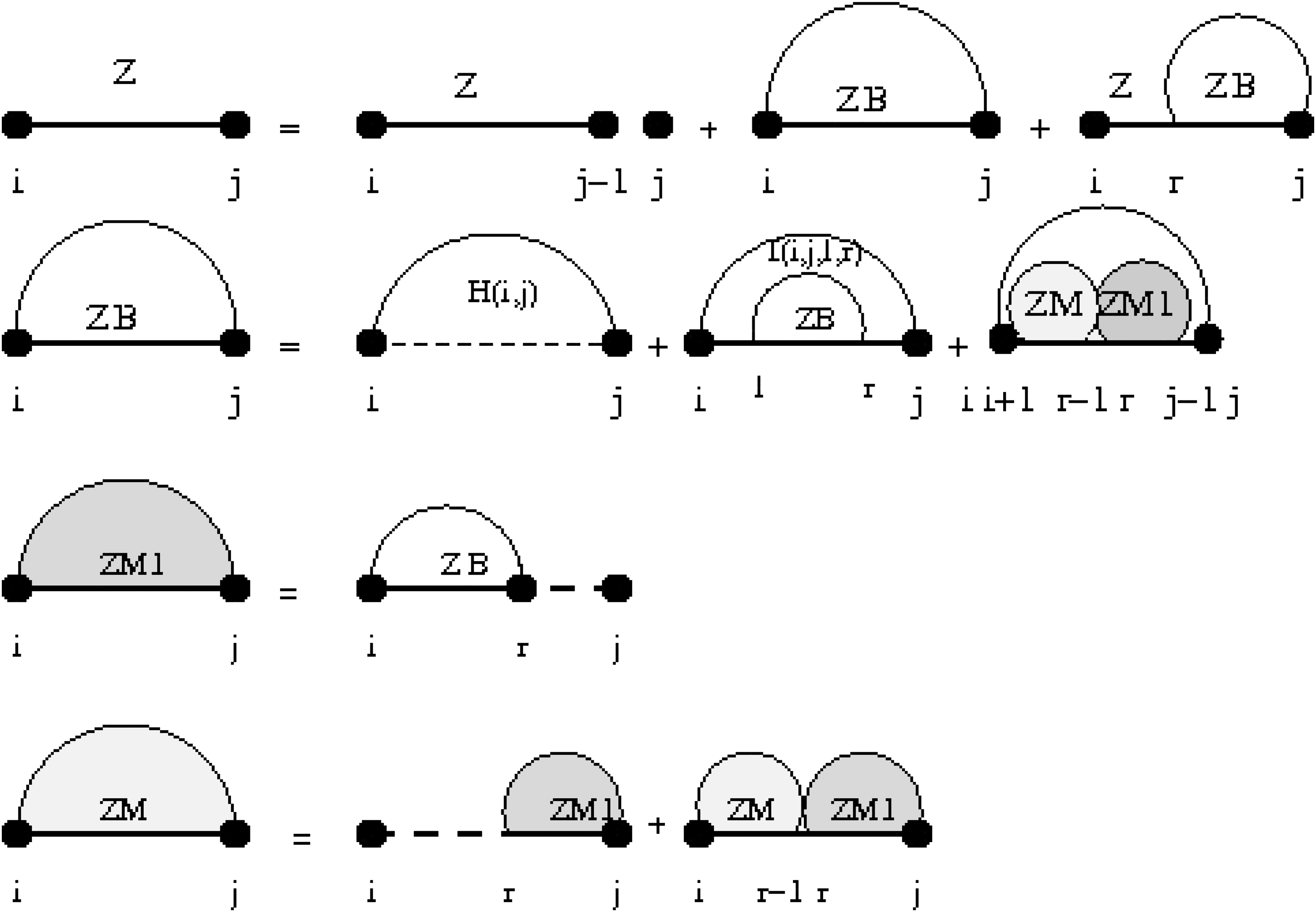
See Figure 1 for a pictorial representation of the recursions of McCaskill's (original) algorithm (McCaskill, 1990); note that the recursions are are not quite the same as those given in Hofacker et al. (1994). We now turn to our parametric versions of the partition function.
Feynman diagram of original recursions from McCaskill's algorithm (McCaskill, 1990) to compute the partition function. Dashed lines present intervals of unpaired bases and shaded arcs represent structures in which i and j will not necessarily pair.
4. Hairpins
We begin by defining some abbreviations for the partition function for hairpins
\documentclass{aastex}\usepackage{amsbsy}\usepackage{amsfonts}\usepackage{amssymb}\usepackage{bm}\usepackage{mathrsfs}\usepackage{pifont}\usepackage{stmaryrd}\usepackage{textcomp}\usepackage{portland, xspace}\usepackage{amsmath, amsxtra}\pagestyle{empty}\DeclareMathSizes{10}{9}{7}{6}\begin{document}
\begin{align*}ZH ( i , j ) = \begin{cases}0 \qquad \qquad \qquad { \rm if} \ j - i \leq \theta \\ e^{ - { \cal H} ( i , j ) / RT} \quad \quad \ { \rm else}\end{cases}\end{align*}
\end{document}
and internal loops having h hairpins
\documentclass{aastex}\usepackage{amsbsy}\usepackage{amsfonts}\usepackage{amssymb}\usepackage{bm}\usepackage{mathrsfs}\usepackage{pifont}\usepackage{stmaryrd}\usepackage{textcomp}\usepackage{portland, xspace}\usepackage{amsmath, amsxtra}\pagestyle{empty}\DeclareMathSizes{10}{9}{7}{6}\begin{document}
\begin{align*}ZI^h ( i , j ) = \sum_{i \leq k \leq \ell \leq j} e^{ - { \cal I} ( i , j;k , l ) / RT} \cdot ZB^h ( k , \ell )\end{align*}
\end{document}
where the sum is over k, ℓ such that (k − i) + (j − ℓ) > 0. This combines the treatment of both left and right bulges with proper internal loops.
For h ≥ 0, define the base cases Zh(i, i) = 1, ZBh(i, i) = ZMh(i, i) = ZM1h(i, i) = 0. The unconstrained partition function for secondary structures restricted to the interval [i, j] that contain h hairpins is given by
\documentclass{aastex}\usepackage{amsbsy}\usepackage{amsfonts}\usepackage{amssymb}\usepackage{bm}\usepackage{mathrsfs}\usepackage{pifont}\usepackage{stmaryrd}\usepackage{textcomp}\usepackage{portland, xspace}\usepackage{amsmath, amsxtra}\pagestyle{empty}\DeclareMathSizes{10}{9}{7}{6}\begin{document}
\begin{align*}Z^h ( i , j ) = \begin{cases}1 \qquad \qquad \qquad
\qquad \qquad \qquad \qquad \qquad \qquad \qquad \qquad \qquad{
\rm if} \ h = 0 \\ Z^h ( i , j - 1 ) + \sum_{r = i}^{j - \theta -
1} \sum_{h_0 + h_1 = h} Z^{h_0} ( i , r - 1 ) ZB^{h_1} ( r , j )
\quad { \rm if} \ h > 0.\end{cases}\end{align*}
\end{document}
The partition function for secondary structures restricted to the interval [i, j] that contains h hairpins and are closed by the base pair (i, j) is given by ZBh(i, j) = 0, if h = 0; ZBh(i, j) = ZH(i, j) + ZIh(i, j), if h = 1; and for h ≥ 2 by
\documentclass{aastex}\usepackage{amsbsy}\usepackage{amsfonts}\usepackage{amssymb}\usepackage{bm}\usepackage{mathrsfs}\usepackage{pifont}\usepackage{stmaryrd}\usepackage{textcomp}\usepackage{portland, xspace}\usepackage{amsmath, amsxtra}\pagestyle{empty}\DeclareMathSizes{10}{9}{7}{6}\begin{document}
\begin{align*}ZB^h ( i , j ) = ZI^h ( i , j ) + \sum_{r = i + \theta + 3}^{j - \theta - 2} \sum_{k = 1}^{h - 1} ZM^{k} ( i + 1 , r - 1 ) \cdot ZM1^{h - k} ( r , j - 1 ) \cdot e^{ - ( a + b ) / RT}.\end{align*}
\end{document}
The multiloop partition function with a single component, and where position i is required to base-pair in the interval [i, j], is given by
\documentclass{aastex}\usepackage{amsbsy}\usepackage{amsfonts}\usepackage{amssymb}\usepackage{bm}\usepackage{mathrsfs}\usepackage{pifont}\usepackage{stmaryrd}\usepackage{textcomp}\usepackage{portland, xspace}\usepackage{amsmath, amsxtra}\pagestyle{empty}\DeclareMathSizes{10}{9}{7}{6}\begin{document}
\begin{align*}ZM1^{h} ( i , j ) = \sum_{r = i + \theta + 1}^j
ZB^h ( i , r ) \cdot e^{ - c ( j - r ) / RT} . \tag{5}\end{align*}
\end{document}
Finally, the multiloop partition function with one or more components, having no requirement that position i base-pair in the interval [i, j], is given by
\documentclass{aastex}\usepackage{amsbsy}\usepackage{amsfonts}\usepackage{amssymb}\usepackage{bm}\usepackage{mathrsfs}\usepackage{pifont}\usepackage{stmaryrd}\usepackage{textcomp}\usepackage{portland, xspace}\usepackage{amsmath, amsxtra}\pagestyle{empty}\DeclareMathSizes{10}{9}{7}{6}\begin{document}
\begin{align*}ZM^{h} ( i , j ) = & \sum_{r = i}^{j - \theta - 1}
ZM1^{h} ( r , j ) \cdot e^{ - ( b + c ( r - i ) ) / RT} & ( 6 ) \\
& + \sum_{r = i + \theta + 2}^{j - \theta - 1} \sum_{k = 1}^{h -
1} ZM^{k} ( i , r - 1 ) \cdot ZM1^{h - k} ( r , j ) \cdot e^{ - b
/ RT}\end{align*}
\end{document}
5. Number Of Multiloops
As before, define the abbreviations for the partition function for hairpins
\documentclass{aastex}\usepackage{amsbsy}\usepackage{amsfonts}\usepackage{amssymb}\usepackage{bm}\usepackage{mathrsfs}\usepackage{pifont}\usepackage{stmaryrd}\usepackage{textcomp}\usepackage{portland, xspace}\usepackage{amsmath, amsxtra}\pagestyle{empty}\DeclareMathSizes{10}{9}{7}{6}\begin{document}
\begin{align*}ZH ( i , j ) = \begin{cases}0 \qquad \qquad \qquad
\ { \rm if} \ j - i \leq \theta \\ e^{ - { \cal H} ( i , j ) / RT}
\qquad \enspace \, { \rm else}\end{cases}\end{align*}
\end{document}
and internal loops having k multiloops
\documentclass{aastex}\usepackage{amsbsy}\usepackage{amsfonts}\usepackage{amssymb}\usepackage{bm}\usepackage{mathrsfs}\usepackage{pifont}\usepackage{stmaryrd}\usepackage{textcomp}\usepackage{portland, xspace}\usepackage{amsmath, amsxtra}\pagestyle{empty}\DeclareMathSizes{10}{9}{7}{6}\begin{document}
\begin{align*}ZI^m ( i , j ) = \sum_{i \leq k \leq \ell \leq j}
e^{ - { \cal I} ( i , j;k , l ) / RT} \cdot ZB^m ( k , \ell
)\end{align*}
\end{document}
where the sum is over k, ℓ such that (k − i) + (j − ℓ)>0. As in the previous section, this combines the treatment of both left and right bulges with proper internal loops.
Define Z0(i, i) = 1, and for m > 0, define Zm(i, i) = 0. For the remaining base cases, define ZBm(i, i) = ZMm(i, i) = ZM1m(i, i) = 0. The unconstrained partition function for secondary structures restricted to the interval [i, j] that contain m multiloops is given by
\documentclass{aastex}\usepackage{amsbsy}\usepackage{amsfonts}\usepackage{amssymb}\usepackage{bm}\usepackage{mathrsfs}\usepackage{pifont}\usepackage{stmaryrd}\usepackage{textcomp}\usepackage{portland, xspace}\usepackage{amsmath, amsxtra}\pagestyle{empty}\DeclareMathSizes{10}{9}{7}{6}\begin{document}
\begin{align*}Z^m ( i , j ) = Z^m ( i , j - 1 ) + \sum_{r = i}^{j
- \theta - 1} \sum_{k = 0}^m Z^k ( i , r - 1 ) \cdot ZB^{m - k} (
r , j )\end{align*}
\end{document}
The partition function for secondary structures restricted to the interval [i, j] that contain m multiloops and are closed by the base pair (i, j) is given by ZBm(i, j) = ZIm(i, j), if m = 0, and in the case that m > 0 and i, j can form a base pair by
\documentclass{aastex}\usepackage{amsbsy}\usepackage{amsfonts}\usepackage{amssymb}\usepackage{bm}\usepackage{mathrsfs}\usepackage{pifont}\usepackage{stmaryrd}\usepackage{textcomp}\usepackage{portland, xspace}\usepackage{amsmath, amsxtra}\pagestyle{empty}\DeclareMathSizes{10}{9}{7}{6}\begin{document}
\begin{align*}ZB^m ( i , j ) = ZI^m ( i , j ) + \sum_{r = i +
\theta + 3}^{j - \theta - 2} \sum_{k = 0}^{m - 1} ZM^{k} ( i + 1 ,
r - 1 ) \cdot ZM1^{m - k - 1} ( r , j - 1 ) \cdot e^{ - ( a + b )
/ RT}.\end{align*}
\end{document}
The multiloop partition function with a single component, and where position i is required to base-pair in the interval [i, j], is given by
\documentclass{aastex}\usepackage{amsbsy}\usepackage{amsfonts}\usepackage{amssymb}\usepackage{bm}\usepackage{mathrsfs}\usepackage{pifont}\usepackage{stmaryrd}\usepackage{textcomp}\usepackage{portland, xspace}\usepackage{amsmath, amsxtra}\pagestyle{empty}\DeclareMathSizes{10}{9}{7}{6}\begin{document}
\begin{align*}ZM1^{m} ( i , j ) = \sum_{r = i + \theta + 1}^j
ZB^m ( i , r ) \cdot e^{ - c ( j - r ) / RT} . \tag{7}\end{align*}
\end{document}
Finally, the multiloop partition function with one or more components, having no requirement that position i base-pair in the interval [i, j] is given by
\documentclass{aastex}\usepackage{amsbsy}\usepackage{amsfonts}\usepackage{amssymb}\usepackage{bm}\usepackage{mathrsfs}\usepackage{pifont}\usepackage{stmaryrd}\usepackage{textcomp}\usepackage{portland, xspace}\usepackage{amsmath, amsxtra}\pagestyle{empty}\DeclareMathSizes{10}{9}{7}{6}\begin{document}
\openup3pt\begin{align*}ZM^{m} ( i , j ) = & \sum_{r = i}^{j - \theta - 1} ZM1^{m} ( r , j ) \cdot e^{ - ( b + c ( r - i ) ) / RT} & ( 8 ) \\ & + \sum_{r = i + \theta + 2}^{j - \theta - 1} \sum_{k = 1}^{m - 1} ZM^{k} ( i , r - 1 ) \cdot ZM1^{m - k - 1} ( r , j ) \cdot e^{ - b / RT}\end{align*}
\end{document}
6. Multiloop Order
The order (or depth) of a secondary structure is the maximum depth of nesting of its multiloops. Formally, multiloop order can be defined via a finite analogue of the Cantor-Bendixson topological derivative (Clote, 1984; Kechris, 1995). The derivative\documentclass{aastex}\usepackage{amsbsy}\usepackage{amsfonts}\usepackage{amssymb}\usepackage{bm}\usepackage{mathrsfs}\usepackage{pifont}\usepackage{stmaryrd}\usepackage{textcomp}\usepackage{portland, xspace}\usepackage{amsmath, amsxtra}\pagestyle{empty}\DeclareMathSizes{10}{9}{7}{6}\begin{document}
$$D ( { \cal S} )$$
\end{document} of secondary structure \documentclass{aastex}\usepackage{amsbsy}\usepackage{amsfonts}\usepackage{amssymb}\usepackage{bm}\usepackage{mathrsfs}\usepackage{pifont}\usepackage{stmaryrd}\usepackage{textcomp}\usepackage{portland, xspace}\usepackage{amsmath, amsxtra}\pagestyle{empty}\DeclareMathSizes{10}{9}{7}{6}\begin{document}
$${ \cal S}$$
\end{document} is equal to the set of base pairs \documentclass{aastex}\usepackage{amsbsy}\usepackage{amsfonts}\usepackage{amssymb}\usepackage{bm}\usepackage{mathrsfs}\usepackage{pifont}\usepackage{stmaryrd}\usepackage{textcomp}\usepackage{portland, xspace}\usepackage{amsmath, amsxtra}\pagestyle{empty}\DeclareMathSizes{10}{9}{7}{6}\begin{document}
$$( i , j ) \in { \cal S}$$
\end{document}, within which there is an internal branching, that is,
\documentclass{aastex}\usepackage{amsbsy}\usepackage{amsfonts}\usepackage{amssymb}\usepackage{bm}\usepackage{mathrsfs}\usepackage{pifont}\usepackage{stmaryrd}\usepackage{textcomp}\usepackage{portland, xspace}\usepackage{amsmath, amsxtra}\pagestyle{empty}\DeclareMathSizes{10}{9}{7}{6}\begin{document}
\begin{align*}D ( { \cal S} ) = \{ ( i , j ) \in { \cal S} : \hbox {there exist distinct} \ ( x , y ) , ( u , v ) \in { \cal S} \ \hbox {such that} \ i < x < y < u < v < j \} .\end{align*}
\end{document}
The order of a secondary structure \documentclass{aastex}\usepackage{amsbsy}\usepackage{amsfonts}\usepackage{amssymb}\usepackage{bm}\usepackage{mathrsfs}\usepackage{pifont}\usepackage{stmaryrd}\usepackage{textcomp}\usepackage{portland, xspace}\usepackage{amsmath, amsxtra}\pagestyle{empty}\DeclareMathSizes{10}{9}{7}{6}\begin{document}
$${ \cal S}$$
\end{document} is now defined to be n − 1, where n is the least integer such that \documentclass{aastex}\usepackage{amsbsy}\usepackage{amsfonts}\usepackage{amssymb}\usepackage{bm}\usepackage{mathrsfs}\usepackage{pifont}\usepackage{stmaryrd}\usepackage{textcomp}\usepackage{portland, xspace}\usepackage{amsmath, amsxtra}\pagestyle{empty}\DeclareMathSizes{10}{9}{7}{6}\begin{document}
$$D ( { \cal S} ) = \emptyset$$
\end{document}. For readers familiar with the notion of RNA shape (Giegerich et al., 2004), it follows that the order of a helix is zero, with shape [ ], while the order of a tRNA cloverleaf secondary structure is one, with shape [ [ ] [ ] [ ] ]. Examples of order 2 secondary structures, with shape [ [ [ ] [ ] [ ] ] [ ] ], are furnished by certain RNase P RNA molecules, such as strand database (Andronescu et al., 2008) sequence ASE00001 from Acidianus ambivalens, and by some transfer-messenger RNA, such as strand database sequence TMR00040, from Azos.oryz.
For typographic reasons, we denote the multiloop partition function by Zd, rather than Zo. As before, define the partition function for hairpins
\documentclass{aastex}\usepackage{amsbsy}\usepackage{amsfonts}\usepackage{amssymb}\usepackage{bm}\usepackage{mathrsfs}\usepackage{pifont}\usepackage{stmaryrd}\usepackage{textcomp}\usepackage{portland, xspace}\usepackage{amsmath, amsxtra}\pagestyle{empty}\DeclareMathSizes{10}{9}{7}{6}\begin{document}
\begin{align*}ZH ( i , j ) = \begin{cases}0 \qquad \qquad \quad { \rm if} \ j - i \leq \theta \\ e^{ - { \cal H} ( i , j ) / RT} \quad \ { \rm else}\end{cases}\end{align*}
\end{document}
and internal loops having multiloop order or depth d\documentclass{aastex}\usepackage{amsbsy}\usepackage{amsfonts}\usepackage{amssymb}\usepackage{bm}\usepackage{mathrsfs}\usepackage{pifont}\usepackage{stmaryrd}\usepackage{textcomp}\usepackage{portland, xspace}\usepackage{amsmath, amsxtra}\pagestyle{empty}\DeclareMathSizes{10}{9}{7}{6}\begin{document}
\begin{align*}ZI^d ( i , j ) = \sum_{i \leq k \leq \ell \leq j} e^{ - { \cal I} ( i , j;k , \ell ) / RT} \cdot ZB^d ( k , \ell )\end{align*}
\end{document}
where the sum is over k, ℓ such that (k − i) + (j − ℓ) > 0. Define Z0(i, i) = 1 and for d > 0, define Zd(i, i) = 0. For d ≥ 0, define ZBd(i, i) = ZMd(i, i) = ZM1d(i, i) = 0. The unconstrained partition function for secondary structures of multiloop order d, when restricted to the interval [i, j], is given by
\documentclass{aastex}\usepackage{amsbsy}\usepackage{amsfonts}\usepackage{amssymb}\usepackage{bm}\usepackage{mathrsfs}\usepackage{pifont}\usepackage{stmaryrd}\usepackage{textcomp}\usepackage{portland, xspace}\usepackage{amsmath, amsxtra}\pagestyle{empty}\DeclareMathSizes{10}{9}{7}{6}\begin{document}
\begin{align*}Z^d ( i , j ) = Z^d ( i , j - 1 ) + \sum_{r = i}^{j - \theta - 1} \quad \sum_{0 \leq k , \ell \leq d , \max ( k , \ell ) = d} Z^k ( i , r - 1 ) \cdot ZB^ \ell ( r , j )\end{align*}
\end{document}
The partition function for secondary structures of multiloop order d when restricted to the interval [i, j] and are closed by the base pair (i, j) is given as follows. For d = 0, let
\documentclass{aastex}\usepackage{amsbsy}\usepackage{amsfonts}\usepackage{amssymb}\usepackage{bm}\usepackage{mathrsfs}\usepackage{pifont}\usepackage{stmaryrd}\usepackage{textcomp}\usepackage{portland, xspace}\usepackage{amsmath, amsxtra}\pagestyle{empty}\DeclareMathSizes{10}{9}{7}{6}\begin{document}
\begin{align*}ZB^d ( i , j ) = ZH ( i , j ) + ZI^d ( i , j )\end{align*}
\end{document}
while for d > 0, define
\documentclass{aastex}\usepackage{amsbsy}\usepackage{amsfonts}\usepackage{amssymb}\usepackage{bm}\usepackage{mathrsfs}\usepackage{pifont}\usepackage{stmaryrd}\usepackage{textcomp}\usepackage{portland, xspace}\usepackage{amsmath, amsxtra}\pagestyle{empty}\DeclareMathSizes{10}{9}{7}{6}\begin{document}
\begin{align*}ZB^d ( i , j ) = & ZI^d ( i , j ) + \sum_{r = i + \theta + 3}^{j - \theta - 1} \ \sum_{0 \leq k , \ell \leq d , \max ( k , \ell ) = d} \\ & ZM^k ( i + 1 , r - 1 ) \cdot ZM1^ \ell ( r , j - 1 ) \cdot e^{ - ( a + b ) / RT}.\end{align*}
\end{document}
The multiloop partition function with a single component, and where position i is required to base-pair in the interval [i, j], is given by
\documentclass{aastex}\usepackage{amsbsy}\usepackage{amsfonts}\usepackage{amssymb}\usepackage{bm}\usepackage{mathrsfs}\usepackage{pifont}\usepackage{stmaryrd}\usepackage{textcomp}\usepackage{portland, xspace}\usepackage{amsmath, amsxtra}\pagestyle{empty}\DeclareMathSizes{10}{9}{7}{6}\begin{document}
\begin{align*}ZM1^{d} ( i , j ) = \sum_{r = i + \theta + 1}^j ZB^d ( i , r ) \cdot e^{ - c ( j - r ) / RT}. \tag{9}\end{align*}
\end{document}
Finally, the multiloop partition function with one or more components, having no requirement that position i base-pair in the interval [i, j], is given by
\documentclass{aastex}\usepackage{amsbsy}\usepackage{amsfonts}\usepackage{amssymb}\usepackage{bm}\usepackage{mathrsfs}\usepackage{pifont}\usepackage{stmaryrd}\usepackage{textcomp}\usepackage{portland, xspace}\usepackage{amsmath, amsxtra}\pagestyle{empty}\DeclareMathSizes{10}{9}{7}{6}\begin{document}
\begin{align*}ZM^{d} ( i , j ) = & \sum_{r = i}^{j - \theta - 1} ZM1^{d} ( r , j ) \cdot e^{ - ( b + c ( r - i ) ) / RT} & ( 10 ) \\ & + \sum_{r = i + \theta + 2}^{j - \theta - 1} \sum_{0 \leq k , \ell \leq d , \max ( k , \ell ) = d} ZM^{k} ( i , r - 1 ) \cdot ZM1^{ \ell} ( r , j ) \cdot e^{ - b / RT}.\end{align*}
\end{document}
7. Simultaneous Multiloop Number and Hairpin Number
Given the algorithms described in Sections 4 and 5, it is straightforward to design the algorithm RNAmloopHP, which computes the partition function Z(m, h) simultaneously for m multiloops and h hairpins. Sampling low-energy structures is done by a straightforward variation of the sampling method introduced by Ding and Lawrence (2003). For purposes of brevity, further details of the partition function and sampling will not be discussed, though the interested reader can study our publicly available source code.
8. Applications
In this section, we mention two main applications of the new algorithms, though first we mention that RNAhairpin presents a novel method to generate suboptimal secondary structures.
In the literature, there are a number of approaches to compute suboptimal secondary structures. Historically, the first method was produced by Zuker (1989), as implemented in mfold mfold (Zuker, 1989) and Unafold (Markham and Zuker, 2008), who for certain base pairs (i, j) computed the minimum free energy structure containing (i, j) that was sufficiently distinct from previously generated suboptimal structures. Next, the program RNAsubopt of Wuchty et al. (1999) generated all secondary structures within a user-specified energy above the minimum free energy. In contrast, the program Sfold (Ding and Lawrence, 2003) samples from the low-energy Boltzmann ensemble of structures; indeed, our implementation of sampling in RNAhairpin is a modification of the method of Ding and Lawrence (2003). [Note that the Sfold algorithm is implemented in the Vienna RNA Package program RNAsubopt with flag −p, as well as the program RNAstructure (Mathews et al., 2004) also supports sampling.] The program RNAshapes of Steffen et al. (2006) computes the minimum free-energy structure from each shape class. The program RNAbor of Freyhult et al. (2007) computes, for each k, the minimum free-energy structure MFE(k) having base-pair distance k from a user-specified reference structure, while the program RNA2Dfold of Lorenz et al. (2009) computes, for each k, ℓ, the minimum free-energy structure MFE(k, ℓ) having base-pair distance k (resp. ℓ) from a first (resp. second) user-specified reference structure. The program RNAlocopt of Lorenz and Clote (2011) samples low locally optimal secondary structures, where a locally optimal structure has the property that its free energy cannot be lowered by the addition or removal of a single base pair. The program RNAbormea of Clote et al. (2012) determines for each k, the maximum expected accuracy structure among all structures having base-pair distance k from a user-specified reference structure. To this list of previous methods, RNAhairpin generates suboptimal secondary structures in a manner that seems orthogonal to previous methods.
8.1. Improved structure prediction for certain RNA families
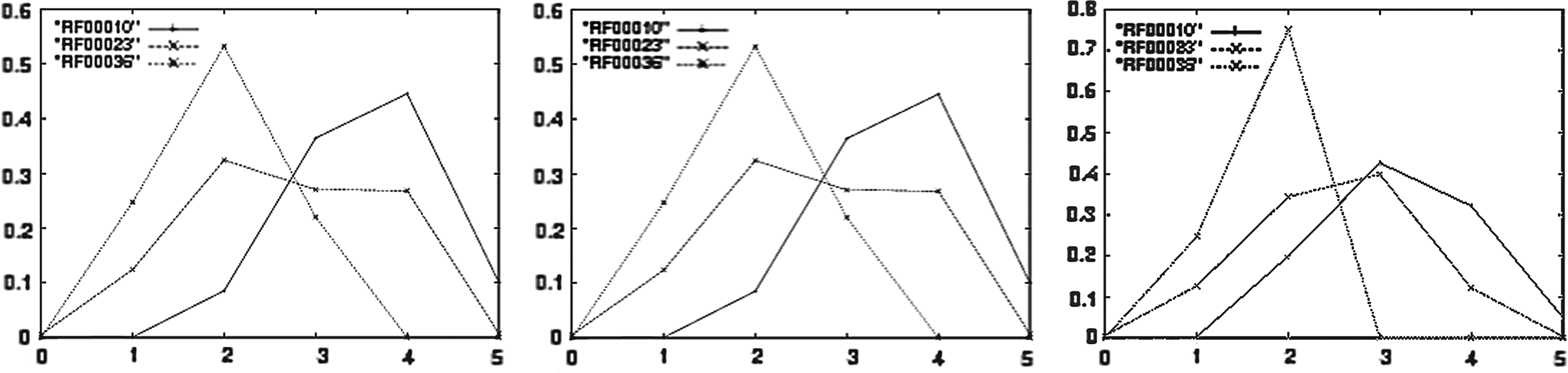
Certain RNAs have a characteristic structure that is important for their function. For instance, the cloverleaf structure of transfer RNA generally has three hairpins, which then form an L-shaped tertiary structure by additional pseudoknots. Transfer RNAs usually contain a small number of chemically modified nucleotides, making their structure at times difficult to predict using minimum free-energy structure methods. In such cases, RNAhairpin (resp., and especially RNAmloopHP) can improve structure prediction by sampling low-energy structures that are required to have a specific number of hairpins (resp. number m of multiloops and h of hairpins). Indeed, Figure 2 displays the average propensity of certain RNA sequences to form a given number of hairpins (resp. given number of multiloops; resp. given order of multiloops) for various Rfam families.
(Left) Hairpin profile of Rfam families: U2 spliceosomal RNA (RF00004), transfer RNA (tRNA, RF00005), and U4 spliceosomal RNA (RF00015). (Center) Multiloop number profile of Rfam families: RNaseP (RF00010), transfer messenger RNA (tmRNA, RF00023), and Rev response element of HIV env gene (RF00036). (Right) Multiloop order (or depth) profile of Rfam families: RNaseP (RF00010), transfer messenger RNA (tmRNA, RF00023), and Rev response element of HIV env gene (RF00036). Notice that we chose Rfam families consisting of long RNA sequences for multiloop number/order profiles, since multiloops are energetically unfavorable, hence, are not generally present in small RNA.
Table 1 presents a comparison of RNAhairpin and RNAfold statistics for sequences taken from the seed alignments of several families from Rfam 11.0 (Burge et al., 2013) (August 2012, 2208 families). For each sequence, we sampled only one low-energy structure having H hairpins. For a given sequence and structure computed either by RNAhairpin or RNAfold, the sensitivity, or true positive rate, is computed, defined as the ratio of the number of correctly predicted base pairs in the Rfam structure over the number of base pairs in the Rfam structure. The average and standard deviation of sensitivity is given, for each Rfam family of the table, for both RNAhairpin and RNAstructure. For these computations, version 1.8.5 of RNAfold was used without dangles, so that both RNAhairpin and RNAfold employed the same energy model. In future work, we plan to lift RNAhairpin to the Turner 2004 energy model and implement dangles, which then would support the same energy model as version 2.0 and higher of RNAfold (Lorenz et al., 2011).
Comparison Between RNAhairpin and RNAfold of the Average Sensitivity (Ratio of Number of Correctly Predicted Base Pairs in Rfam Structure over Number of Base Pairs in Rfam Structure) for Various Rfam Families
RNA family
H
RNAhairpin μ ± σ
RNAfold μ ± σ
Avg len
Num seq
RF00001
2
0.6213 ± 0.2667
0.6332 ± 0.2721
116.6
712
RF00004
5
0.7548 ± 0.1840
0.7104 ± 0.2058
190.5
208
RF00005
3
0.7345 ± 0.2313
0.5370 ± 0.1992
73.4
960
RF00008
2
0.9565 ± 0.1284
0.9154 ± 0.1894
55.4
84
RF00031
1
0.7679 ± 0.1748
0.7657 ± 0.1945
64.5
61
RF00045
4
0.4420 ± 0.2983
0.4205 ± 0.3274
202.6
66
RF00094
2
0.3080 ± 0.2131
0.3604 ± 0.2091
91.1
33
RF00167
2
0.8113 ± 0.2301
0.8568 ± 0.2290
100.8
133
RF00375
2
0.8278 ± 0.3060
0.8814 ± 0.2044
99.0
130
RF00504
2
0.5940 ± 0.2711
0.5603 ± 0.2895
100.9
44
RF00635
4
0.3024 ± 0.1127
0.3707 ± 0.1204
117.9
13
RF01055
4
0.5821 ± 0.2725
0.5787 ± 0.2641
142.0
160
RNAhairpin was used to sample a single secondary structure having H many hairpins, and the average sensitivity of RNAhairpin and RNAfold was computed over all sequences in the seed alignment of the following Rfam families: RF00001 (5S rRNA), RF00004 (splicesomal U2 RNA), RF00005 (tRNA), RF00008 (type III hammerhead ribozyme), RF00031 (selenocysteine insertion sequence I), RF00045 (snoRNA), RF00094 (HDV ribozyme), RF00167 (purine riboswitch), RF00375 (HIV primer binding site), RF00504 (glycine riboswitch), RF00635 (HAR1A), and RF01055 (moco RNA motif).
In the case of tRNA, there is more than 20% improvement in sensitivity of RNAhairpin over RNAfold; RNAhairpin has greater sensitivity than RNAfold for other instances, such as in the case of the hammerhead ribozyme (around 4% improvement). On the other hand, RNAfold has greater sensitivity than RNAhairpin for several classes, including HIV primer binding site RF00375 (over 5% improvement), and purine riboswitch aptamers RF00167 (around 4.5% improvement). Clearly RNAhairpin is not a better structure prediction tool than RNAfold; however, for particular classes of functional RNA, which require certain hairpin structures for function, RNAhairpin may provide a useful tool. (See Section 9 for more discussion.)
As shown in Table 2, the program RNAmloopHP, which samples low-energy structures having m multiloops and h hairpins, improves the structure prediction accuracy of RNAhairpin (e.g., an improvement of over 4% for RF000167 purine riboswitches), and also outperforms RNAfold for a larger number of cases on the previously described Rfam families. For instance, there is an improvement of almost 24% in RF00005 (tRNA), over 4% in RF00008 (type III hammerhead ribozyme), 5% in RF00504 (glycine riboswitch), and so on. On the other hand, RNAmloopHP has significantly lower sensitivity than RNAfold in the following two cases, where the difference is over 5% for RF00375 (HIV primer binding site), and 8% for RF00635 (HAR1A). The consensus structures for these Rfam families have large loop regions, which may in fact be base-paired, which could explain the poorer performance of RNAmloopHP. (Recall that Rfam consensus structures are determined by covariation found in multiple alignments, thus loop regions in consensus structures could indeed be base-paired and involve additional hairpins and/or multiloops.) In any case, we do not propose the use of RNAmloopHP in place of minimum free-energy structure software, such as RNAfold; instead, if a biologist has knowledge or intuition about the existence of a certain number of multiloops and hairpins, then RNAmloopHP may prove to be a useful tool.
Comparison Between RNAmloopHP and RNAfold of the Average Sensitivity for the Same Rfam Families, as inTable 1.
RNA family
M
H
RNAhairpin μ ± σ
RNAfold μ ± σ
Avg len
Num seq
RF00001
1
2
0.6308 ± 0.2571
0.6332 ± 0.2721
116.6
712
RF00004
0
5
0.6980 ± 0.1780
0.7104 ± 0.2058
190.5
208
RF00005
1
3
0.7740 ± 0.1946
0.5370 ± 0.1992
73.4
960
RF00008
1
2
0.9582 ± 0.1005
0.9154 ± 0.1894
55.4
84
RF00031
0
1
0.7679 ± 0.1748
0.7657 ± 0.1945
64.5
61
RF00045
1
4
0.4456 ± 0.2977
0.4205 ± 0.3274
202.6
66
RF00094
0
2
0.3464 ± 0.1951
0.3604 ± 0.2091
91.1
33
RF00167
1
2
0.8511 ± 0.1726
0.8568 ± 0.2290
100.8
133
RF00375
1
2
0.8283 ± 0.3063
0.8814 ± 0.2044
99.0
130
RF00504
1
2
0.6101 ± 0.264
0.5603 ± 0.2895
100.9
44
RF00635
1
3
0.2930 ± 0.1059
0.3707 ± 0.1204
117.9
13
RF01055
1
4
0.60170 ± 0.277
0.5787 ± 0.2641
142.0
160
By now sampling a single secondary structure having simultaneously M many multiloops and H many hairpins, the average sensitivity improved over that of RNAhairpin in essentially all cases. Moreover, RNAmloopHP provides more accurate structure prediction (sensitivity) than RNAfold for a number of Rfam families. There is an improvement of almost approx24% in RF00005 (tRNA), more than 4% in RF00008 (type III hammerhead ribozyme), 2.5% in RF00045 (snoRNA), 5% in RF00504 (glycine riboswitch), and more than 2% in RF01055 (moco RNA motif). On the other hand, RNAmloopHP has significantly lower sensitivity than RNAfold in the following two cases, where the difference is over 5% for RF00375 (HIV primer binding site), and 8% for RF00635 (HAR1A). Insignificant differences, such as 0.6308 for RNAmloopHP versus 0.6332 in RF00001 (5S rRNA), are likely to be due to the stochastic nature of sampling low-energy structures, rather than computing the MFE structure having a specified number of multiloops and hairpins.
8.2. Support vector machine results
In this section, we describe receiver operating characteristic (ROC) curves, computed by five-fold cross-validation, where in each case, the positive instances were taken to be sequences from the seed alignment of a given Rfam family, and negative instances were taken to be random sequences having the same number of dinucleotides, as computed by our implementation of the Altschul-Erikson algorithm (Altschul and Erikson, 1985). (Similar results were obtained when we took negative instances to be sequences the seed alignments of all other Rfam families—data not shown.)
For each positive instance, we generated 10 random negative instances. Using libSVM (Chang and Lin, 2001), we performed a stratified training by selecting one-fifth of the positive instances together with an equal number of negative instances (one of the 10 negative instances was selected for each positive instance) for training. The remaining four-fifths of the positive sequences, together with all corresponding negative instances, constituted the test set (note that in testing, there were 10 negative instances per positive sequence). A radial basis kernel was chosen with cost C = 1, and parameter γ taken to be the reciprocal of the number of features.
We considered three feature sets: HP, HP/M, and HP/M/O, where HP features were the 21 probabilities of hairpin formation \documentclass{aastex}\usepackage{amsbsy}\usepackage{amsfonts}\usepackage{amssymb}\usepackage{bm}\usepackage{mathrsfs}\usepackage{pifont}\usepackage{stmaryrd}\usepackage{textcomp}\usepackage{portland, xspace}\usepackage{amsmath, amsxtra}\pagestyle{empty}\DeclareMathSizes{10}{9}{7}{6}\begin{document}
$$p_h ( 0 ) , \ldots , p_h ( 20 )$$
\end{document}, where M features were the six probabilities of multiloop formation \documentclass{aastex}\usepackage{amsbsy}\usepackage{amsfonts}\usepackage{amssymb}\usepackage{bm}\usepackage{mathrsfs}\usepackage{pifont}\usepackage{stmaryrd}\usepackage{textcomp}\usepackage{portland, xspace}\usepackage{amsmath, amsxtra}\pagestyle{empty}\DeclareMathSizes{10}{9}{7}{6}\begin{document}
$$p_m ( 0 ) , \ldots , p_m ( 5 )$$
\end{document}, and where O features were the six probabilities of multiloop order (or depth) \documentclass{aastex}\usepackage{amsbsy}\usepackage{amsfonts}\usepackage{amssymb}\usepackage{bm}\usepackage{mathrsfs}\usepackage{pifont}\usepackage{stmaryrd}\usepackage{textcomp}\usepackage{portland, xspace}\usepackage{amsmath, amsxtra}\pagestyle{empty}\DeclareMathSizes{10}{9}{7}{6}\begin{document}
$$p_d ( 0 ) , \ldots , p_d ( 5 )$$
\end{document}. Thus the SVM binary classifier HP (hairpins) has 21 features, though in most cases all but a small number of the features are 0; the classifier HP/M (hairpin and multiloop number) has 27 = 21 + 6 features; the classifier HP/M/O (hairpin, multiloop number, multiloop order) has 33 = 21 + 6 + 6 features. The R packages e1071 (Meyer et al., 2012) and pROC (Robin et al., 2011) were used with libSVM (Chang and Lin, 2001).
Table 3 summarizes the area under the curve (AUC) values for ROC curves of the three different SVM classifiers HP, HP/M, HP/M/O, while Figure 3 depicts the corresponding ROC curves. Note that in all cases, inclusion of multiloop order probabilities as features does not add any discriminatory power, and even in certain cases reduces the AUC. This is fortunate, since RNAmloopOrder cannot be sped up by using the fast Fourier transform, unlike RNAhairpin and RNAmloopNum. The results of this table and figure indicate that, although hairpin and multiloop formation probabilities may not be sufficient to be used solely as the feature set of a noncoding RNA gene finder, we believe that, when added, these features could lead to improvements in performance of existent RNA gene finders. Moreover, to the best of our knowledge, current noncoding RNA gene finders do not take into account global propensity to form hairpins or multiloops.
Receiver operating characteristic (ROC) curves for the performance of support vector machine binary classification using a feature set consisting of probabilities \documentclass{aastex}\usepackage{amsbsy}\usepackage{amsfonts}\usepackage{amssymb}\usepackage{bm}\usepackage{mathrsfs}\usepackage{pifont}\usepackage{stmaryrd}\usepackage{textcomp}\usepackage{portland, xspace}\usepackage{amsmath, amsxtra}\pagestyle{empty}\DeclareMathSizes{10}{9}{7}{6}\begin{document}
$$p ( 0 ) , \ldots , p ( 20 )$$
\end{document} for the number hairpins (HP), probabilities \documentclass{aastex}\usepackage{amsbsy}\usepackage{amsfonts}\usepackage{amssymb}\usepackage{bm}\usepackage{mathrsfs}\usepackage{pifont}\usepackage{stmaryrd}\usepackage{textcomp}\usepackage{portland, xspace}\usepackage{amsmath, amsxtra}\pagestyle{empty}\DeclareMathSizes{10}{9}{7}{6}\begin{document}
$$p ( 0 ) , \ldots , p ( 5 )$$
\end{document} for the number of multiloops (M), and probabilities \documentclass{aastex}\usepackage{amsbsy}\usepackage{amsfonts}\usepackage{amssymb}\usepackage{bm}\usepackage{mathrsfs}\usepackage{pifont}\usepackage{stmaryrd}\usepackage{textcomp}\usepackage{portland, xspace}\usepackage{amsmath, amsxtra}\pagestyle{empty}\DeclareMathSizes{10}{9}{7}{6}\begin{document}
$$p ( 0 ) , \ldots , p ( 5 )$$
\end{document} for the maximum order of multiloops (O). In the case of HP (hairpin number), there were 21 features, though in most cases all but at most 6–8 features had the value 0; in the case of HP/M (hairpin and multiloop number), there were 27 = 21 + 6 features; and in the case of HP/M/O (hairpin and multiloop number with maximum multiloop order), there were 33 = 21 + 6 + 6 features. The R packages e1071 (Meyer et al., 2012) and pROC (Robin et al., 2011) were used with libSVM (Chang and Lin, 2001). A radial basis kernel was used in each case with cost C = 1; parameter γ was taken to be the inverse of the number of features, that is, for HP, γ = 1/21 = 0.0476, for HP/M, γ = 1/27 = 0.0370, and for HP/M/O, γ = 1/33 = 0.0303. As shown in this figure, accounting for multiloop order did not improve classification ROC curves, and data presented in Table 3 shows that in some cases, ROC area under the curve is lessened by taking into account maximum multiloop order. This is in fact fortunate, since the fast Fourier transform can be applied to reduce time and space requirements for RNAhairpin and RNAmloopNum but not RNAmloopOrder. (Left) Rfam family RF00004 (U2 spliceosomal RNA). (Right) Rfam family RF00167 (purine riboswitch).
Area Under Curve (AUC) for Receiver Operating Characteristic (ROC) Curves for Seven Rfam Families
Family name and description
H
HM
HMO
Num seq
Avg len
Avg GC %
RF00004 U2 spliceosomal RNA
0.9217
0.9282
0.9328
208
204.26
48.0%
RF00005 tRNA
0.6367
0.9038
0.9017
959
73.4
47.0%
RF00008 hammerhead III
0.9191
0.9705
0.9562
84
55.4
48.4%
RF00027 let 7 microRNA precursor
0.8338
0.8766
0.8617
67
79.6
43.7%
RF00031 SECIS 1
0.7917
0.8361
0.7941
61
64.5
49.0%
RF00045 SNORA73
0.6306
0.6515
0.6609
66
202.6
53.1%
RF00167 purine riboswitch
0.6508
0.8608
0.8529
136
100.8
38.1%
Each family tested under five-fold cross-validation with support vector machines (SVM) using a radial basis kernel with cost C = 1 and γ equal to the inverse of the number of features. In the case of H (hairpin number), there were 21 hairpin formation probabilities \documentclass{aastex}\usepackage{amsbsy}\usepackage{amsfonts}\usepackage{amssymb}\usepackage{bm}\usepackage{mathrsfs}\usepackage{pifont}\usepackage{stmaryrd}\usepackage{textcomp}\usepackage{portland, xspace}\usepackage{amsmath, amsxtra}\pagestyle{empty}\DeclareMathSizes{10}{9}{7}{6}\begin{document}
$$p ( 0 ) , \ldots , p ( 20 )$$
\end{document} taken as features (though in most cases all but a very small number of these probabilities were zero); in the case of HM (hairpin and multiloop number), there were 27 = 21 + 6 hairpin and multiloop formation probabilities taken as features, and in the case of HMO (hairpin and multiloop number with maximum multiloop order), there were 27 = 21 + 6 hairpin and multiloop formation probabilities taken as features along with six multiloop maximum order probabilities, hence altogether 33 = 21 + 6 + 6 features. The R packages e1071 (Meyer et al., 2012) and pROC (Robin et al., 2011) were used with libSVM (Chang and Lin, 2001).
Table 4 presents the ratio of ROC area under the curve values for support vector machines (SVM) over that for relevance vector machines (RVM). A value greater (resp. less) than unity in the table indicates that SVM outperforms (resp. underperforms) RVM using the same features. Figure 4 shows an unexpected situation for the five-fold (stratified) cross-validation experiments of the Rfam family RF00027, using the feature set consisting of only 21 hairpin formation probabilities \documentclass{aastex}\usepackage{amsbsy}\usepackage{amsfonts}\usepackage{amssymb}\usepackage{bm}\usepackage{mathrsfs}\usepackage{pifont}\usepackage{stmaryrd}\usepackage{textcomp}\usepackage{portland, xspace}\usepackage{amsmath, amsxtra}\pagestyle{empty}\DeclareMathSizes{10}{9}{7}{6}\begin{document}
$$p_h ( 0 ) , \ldots , p_h ( 20 )$$
\end{document}, the ratio of SVM/RVM AUC is 1.4234, indicating that SVM far outperforms RVM for this family using these features, while for the full feature set of hairpin formation probabilities \documentclass{aastex}\usepackage{amsbsy}\usepackage{amsfonts}\usepackage{amssymb}\usepackage{bm}\usepackage{mathrsfs}\usepackage{pifont}\usepackage{stmaryrd}\usepackage{textcomp}\usepackage{portland, xspace}\usepackage{amsmath, amsxtra}\pagestyle{empty}\DeclareMathSizes{10}{9}{7}{6}\begin{document}
$$p_h ( 0 ) , \ldots , p_h ( 20 )$$
\end{document}, multiloop number probabilities \documentclass{aastex}\usepackage{amsbsy}\usepackage{amsfonts}\usepackage{amssymb}\usepackage{bm}\usepackage{mathrsfs}\usepackage{pifont}\usepackage{stmaryrd}\usepackage{textcomp}\usepackage{portland, xspace}\usepackage{amsmath, amsxtra}\pagestyle{empty}\DeclareMathSizes{10}{9}{7}{6}\begin{document}
$$p_h ( 0 ) , \ldots , p_h ( 6 )$$
\end{document}, and multiloop maximum order (depth) probabilities \documentclass{aastex}\usepackage{amsbsy}\usepackage{amsfonts}\usepackage{amssymb}\usepackage{bm}\usepackage{mathrsfs}\usepackage{pifont}\usepackage{stmaryrd}\usepackage{textcomp}\usepackage{portland, xspace}\usepackage{amsmath, amsxtra}\pagestyle{empty}\DeclareMathSizes{10}{9}{7}{6}\begin{document}
$$p_h ( 0 ) , \ldots , p_h ( 6 )$$
\end{document}, the ratio of SVM/RVM AUC is 0.8986, indicating that RVM outperforms SVM.
Receiver operating characteristic (ROC) curves for five-fold cross-validation for sequences from the seed alignment of RF00027. The left panel shows an overlay of support vector machine (SVM) and relevance vector machine (RVM) for the feature set consisting of 21 hairpin formation probabilities \documentclass{aastex}\usepackage{amsbsy}\usepackage{amsfonts}\usepackage{amssymb}\usepackage{bm}\usepackage{mathrsfs}\usepackage{pifont}\usepackage{stmaryrd}\usepackage{textcomp}\usepackage{portland, xspace}\usepackage{amsmath, amsxtra}\pagestyle{empty}\DeclareMathSizes{10}{9}{7}{6}\begin{document}
$$p_h ( 0 ) , \ldots , p_h ( 20 )$$
\end{document}, while the right panel presents an overlay of SVM and RVM for the full feature set of hairpin formation probabilities \documentclass{aastex}\usepackage{amsbsy}\usepackage{amsfonts}\usepackage{amssymb}\usepackage{bm}\usepackage{mathrsfs}\usepackage{pifont}\usepackage{stmaryrd}\usepackage{textcomp}\usepackage{portland, xspace}\usepackage{amsmath, amsxtra}\pagestyle{empty}\DeclareMathSizes{10}{9}{7}{6}\begin{document}
$$p_h ( 0 ) , \ldots , p_h ( 20 )$$
\end{document}, multiloop number probabilities \documentclass{aastex}\usepackage{amsbsy}\usepackage{amsfonts}\usepackage{amssymb}\usepackage{bm}\usepackage{mathrsfs}\usepackage{pifont}\usepackage{stmaryrd}\usepackage{textcomp}\usepackage{portland, xspace}\usepackage{amsmath, amsxtra}\pagestyle{empty}\DeclareMathSizes{10}{9}{7}{6}\begin{document}
$$p_h ( 0 ) , \ldots , p_h ( 6 )$$
\end{document}, and multiloop maximum order (depth) probabilities \documentclass{aastex}\usepackage{amsbsy}\usepackage{amsfonts}\usepackage{amssymb}\usepackage{bm}\usepackage{mathrsfs}\usepackage{pifont}\usepackage{stmaryrd}\usepackage{textcomp}\usepackage{portland, xspace}\usepackage{amsmath, amsxtra}\pagestyle{empty}\DeclareMathSizes{10}{9}{7}{6}\begin{document}
$$p_h ( 0 ) , \ldots , p_h ( 6 )$$
\end{document}. As explained in the caption of Table 4, it seems unusual that SVM outperforms RVM using only hairpin probability features, while the reverse is true when using the full feature set.
Ratio of ROC Area Under Curve Values for Two Types of Machine-Learning Methods: Support Vector Machines (SVM) and Relevance Vector Machines (RVM), Using the Same Seven Rfam Families That Were Considered inTable 3
Ratio SVM/RVM
RF00004
RF00005
RF00008
RF00027
RF00031
RF00045
RF00167
HP
0.9874
1.0657
0.9874
1.4234
1.1965
0.9895
1.1894
HP/M
0.9863
0.9798
0.9977
1.0625
1.0954
0.9808
1.0153
HP/M/O
0.9818
0.9855
1.0025
0.8986
1.2324
1.0237
1.0031
In 11 out of 21 tests, AUC values for SVMs were greater than those for RVMs. In the case of RF00027, it is interesting to note that when using only hairpin features, SVM AUC was much higher than RVM AUC (SVM/RVM 1.4234), while for the same class, when using the larger feature set for hairpins, multiloop number, and multiloop order, SVM AUC was lower than RVM AUC (SVM/RVM 0.8986). At present, the reason for this surprising result is unclear. The R packages e1071 (Meyer et al., 2012) and pROC (Robin et al., 2011) were used for SVM and RVM computations; for SVM, the radial basis kernel (rbfkernel) was employed with default parameters, while for RVM, rvmbinary rbfdot kernel was used with default parameters and 1000 iterations.
9. Discussion and Conclusion
We end the article with a discussion of strengths and shortcomings of each application shown: improved structure prediction and support vector machine classification.
9.1. Parametric structure prediction
For benchmarking purposes in Table 1, we sampled only one low-energy structure having H many hairpins, where in most cases H was taken to be the number of hairpins in the Rfam consensus structure of the first member of the Rfam family. This explains how it could happen that the RNAhairpin sensitivity for a certain sequence could at times be different than the RNAhairpin sensitivity for the same sequence, even when the sampled structure and the minimum free-energy structure have the same number of hairpins. Of course, in general, our code RNAhairpin will be used to sample a large number (1,000 or 10,000) of structures per sequence.
Since the base pairs that appear in Rfam consensus structures are inferred by covariation observed in a multiple alignment, many valid base pairs do not appear in the consensus structure. For this reason, we did not compute positive predictive rate, defined as the ratio of the number of correctly predicted base pairs in the Rfam consensus structure divided by the number of base pairs in the predicted structure. This is the reason that Table 1 only reports average sensitivity values.
As previously mentioned, we computed the average sensitivity of the minimum free-energy (MFE) structure obtained from Vienna RNA Package RNAfold (Hofacker, 2003), version 1.8.5 without dangles, to ensure that both RNAhairpin and RNAfold employ the same energy model. In future work, we plan to extend RNAhairpin to the Turner 2004 energy model with dangles (Turner and Mathews, 2009). By the same token, it is not conceptually difficult to modify the program RNAmloopNum to sample low-energy structures having a specified number of multiloops. Such sampled structures could yield better structure predictions for certain types of RNA. Finally, it would be possible to combine the algorithms RNAhairpin and RNAmloopNum in order to sample structures having both a specified number of hairpins and a possibly distinct number of multiloops. Nevertheless, such an algorithm would run in time O(H2M2n3) and space O(HMn2), where H (resp. M) is an upper bound on the number of hairpins (resp. multiloops). For relatively small values of H, M, such an algorithm would indeed be feasible, and could prove useful for certain classes of RNA, whose function is known to depend on certain structural motifs.
Table 1 presents examples of Rfam families, where the average sensitivity of RNAhairpin exceeds that of RNAfold. Improvements were obtained for RNA families, where a certain number of hairpins are known to be functionally important, as in the cloverleaf tRNA, typically having three hairpins. In this case, the sensitivity of RNAhairpin exceeds that of RNAfold by approximately 20%. For certain ribozymes, such as type III hammerhead ribozyme (RF00008) and glycine ribozyme (RF00504), the improvement was over 4% (resp. 3%). Not shown in the table are RNA families, where the sensitivity of RNAfold exceeded that of RNAhairpin—for instance, for 5S rRNA (RF00001), RNAhairpin average sensitivity was 0.621306 compared with RNAfold sensitivity of 0.633189; for purine riboswitches (RF00167), RNAhairpin obtained had 0.811327 compared with RNAfold sensitivity of 0.856764. We believe that RNAhairpin showed better sensitivity than RNAfold in the case of tRNA because of two reasons: (1) tRNA has a well-known cloverleaf structure usually involving three hairpins, and (2) there may be a large sequence and energy difference among especially bacterial tRNAs. Item (2) could cause minimum free-energy structures to be quite distinct from the usual cloverleaf—manual investigation confirms this hypothesis in some randomly chosen instances, while item (2) ensures that RNAhairpin will sample structures having three hairpins, hence more likely to adopt the functional cloverleaf structure. It could be that similar reasons explain the small improvement of RNAhairpin over RNAfold for some of the other examples, including certain ribozymes. However, along this line of reasoning, we expected RNAhairpin to outperform RNAfold for purine riboswitch aptamers, which have a very well-defined multiloop with two hairpins; Table 1 shows this is not the case. As described in the caption of Table 2, by sampling low-energy structures that simultaneously have a specified number m of multiloops and number h of hairpins, we substantially improve the prediction accuracy of RNAfold. However, such improvements tend to occur when the Rfam families show a prounounced common fold, as in the case of tRNA and certain ribozymes, and when there are no large loop (undefined) regions in the Rfam consensus structures. In any case, we believe that minimum free-energy structure prediction algorithms, such as RNAfold, UNAFold, mfold, RNAstructure, remain the best universal thermodynamics-based tool for structure prediction.
9.2. Features for SVM classifiers
The development of noncoding RNA gene finders is important for the analysis and classification of the pervasively transcribed RNA from the human genome, most of which has no previously known structure or function. In this article, we have described four novel thermodynamics-based algorithms—RNAhairpin, RNAmloopNum, RNAmloopOrder, and RNAmloopHP—that compute global, parametric features of the ensemble of low energy secondary structures for a given RNA sequence. For the first three algorithms, we have shown that there is a significant global signal, as witnessed by ROC area under the curve, which suggests that probability and multiloop formation probabilities present useful features that could be added to existent noncoding RNA gene finders—note that this remark only concerns gene finders for specific noncoding RNA families, not general ncRNA gene finders.
One of our goals in developing these parametric algorithms was to provide additional discriminatory features that can be added to other features within the context of a support vector machine, in order to improve the accuracy of noncoding RNA gene finders. Indeed, by adding novel features, it is known that one can improve the accuracy of SVM classifiers. For instance, the state-of-the-art precursor microRNA (pre-miRNA) SVM developed by Ng and Mishra (2007) uses features MFEI2, MFEI1, %G+C, dP, dG, dQ, dD, dF, zG, zQ, zD, zP, zF, and so on. (see Ng and Mishra, 2007, for further explanation), which outperforms the simpler triplet kernel pre-miRNA SVM developed by Xue et al. (2005).
10. Appendix: Using Fft To Compute Rnahairpin
In Freyhult et al. (2007), we developed the algorithm RNAbor, which computes the minimum free energy structure MFE(k) and the partition function Z(k) for each integer k, where Z(k) is the sum of Boltzmann factors exp(−E(S)/RT), and the sum is taken over all structures having base-pair distance k from a user-specified reference structure. Like the parametric algorithms RNAhairpin, RNAmloopNum, and RNAmloopOrder in this article, RNAbor runs in time O(n5) and space O(n3), when all values Z(k) are needed for 0 ≤ k ≤ n.
In Senter et al. (2012), we described a more efficient means to compute the partition functions Z(k) for 0 ≤ k ≤ n by using the FFT to determine probabilities p(k) = Z(k)/Z by polynomial interpolation. Since the partition function Z can be separately computed by McCaskill's algorithm (McCaskill, 1990), the new method yields the values Z(k) for 0 ≤ k ≤ n in time O(n4) and space O(n2).
Given the algorithmic similarities between the parametric algorithms of this article and RNAbor, we can use the same method of polynomial interpolation using the FFT to compute probabilities ph(k) = Zh(k)/Z and pm(k) = Zm(k)/Z for hairpin (resp. multiloop) formation, for all 0 ≤ k ≤ n. For technical reasons having to do with the replacement of summation by taking the maximum, we can not use the FFT to compute probabilities pd(k) for multiloop order (depth). Moreover, although the O(n5) time and O(n3) space algorithms presented in this article can additionally sample low energy structures, the more efficient O(n4) time and O(n2) space algorithms using the FFT can not be used to sample structures—see Senter et al. (2012) for explanation of the analogous situation with a related algorithm using the FFT.
With these remarks, we succinctly describe the overall recursions for the FFT version of RNAhairpin; similar recursions apply to the FFT version of RNAmloopNum. All algorithms described in this article have been implemented and are publicly available at http://bioinformatics.bc.edu/RNAparametric/
10.1. FFT version of RNAhairpin
Let \documentclass{aastex}\usepackage{amsbsy}\usepackage{amsfonts}\usepackage{amssymb}\usepackage{bm}\usepackage{mathrsfs}\usepackage{pifont}\usepackage{stmaryrd}\usepackage{textcomp}\usepackage{portland, xspace}\usepackage{amsmath, amsxtra}\pagestyle{empty}\DeclareMathSizes{10}{9}{7}{6}\begin{document}
$${ \rm s} = s_1 , \ldots , s_n$$
\end{document} be a given RNA sequence. For all 1 ≤ i ≤ j ≤ n, we define the polynomial\documentclass{aastex}\usepackage{amsbsy}\usepackage{amsfonts}\usepackage{amssymb}\usepackage{bm}\usepackage{mathrsfs}\usepackage{pifont}\usepackage{stmaryrd}\usepackage{textcomp}\usepackage{portland, xspace}\usepackage{amsmath, amsxtra}\pagestyle{empty}\DeclareMathSizes{10}{9}{7}{6}\begin{document}
\begin{align*}{ \cal Z}_{i , j} ( x ) = \sum_{k = 0}^{n - 1} z_{i , j} ( k ) \cdot x^k\end{align*}
\end{document}
where zi,j is the hairpin partition function for interval [i, j]; that is, zi,j is the sum of Boltzmann factors exp(−E(S)/RT), taken over all secondary structures S of \documentclass{aastex}\usepackage{amsbsy}\usepackage{amsfonts}\usepackage{amssymb}\usepackage{bm}\usepackage{mathrsfs}\usepackage{pifont}\usepackage{stmaryrd}\usepackage{textcomp}\usepackage{portland, xspace}\usepackage{amsmath, amsxtra}\pagestyle{empty}\DeclareMathSizes{10}{9}{7}{6}\begin{document}
$$s_i , \ldots , s_j$$
\end{document}. Since the coefficients of any polynomial of degree strictly less than n can be efficiently determined by the FFT using polynomial interpolation, provided that one first evaluates the polynomial at n, many complex nth roots of unity 1, \documentclass{aastex}\usepackage{amsbsy}\usepackage{amsfonts}\usepackage{amssymb}\usepackage{bm}\usepackage{mathrsfs}\usepackage{pifont}\usepackage{stmaryrd}\usepackage{textcomp}\usepackage{portland, xspace}\usepackage{amsmath, amsxtra}\pagestyle{empty}\DeclareMathSizes{10}{9}{7}{6}\begin{document}
$$\exp ( \frac { 2 \pi i } { n } ) , \ldots , \exp ( \frac { 2 \pi i ( n - 1 ) } { n } )$$
\end{document}. For a complex number α, in order to evaluate \documentclass{aastex}\usepackage{amsbsy}\usepackage{amsfonts}\usepackage{amssymb}\usepackage{bm}\usepackage{mathrsfs}\usepackage{pifont}\usepackage{stmaryrd}\usepackage{textcomp}\usepackage{portland, xspace}\usepackage{amsmath, amsxtra}\pagestyle{empty}\DeclareMathSizes{10}{9}{7}{6}\begin{document}
$${ \cal Z} ( \alpha ) = { \cal Z}_{1 , n} ( \alpha )$$
\end{document}, we proceed by recursions that somewhat resemble the recursions given in Section 4. To compute Z1,n(α), we use dynamic programming to evaluate Zi,j(α), for all 1 ≤ i ≤ j ≤ n; moreover, in order to compute Zi,j(α), we need to compute ZBi,j(α), ZMi,j(α), and ZM1i,j(α).
Now let B denote the set of canonical base pairs GC, CG, AU, UA, GU, and UG. To compute \documentclass{aastex}\usepackage{amsbsy}\usepackage{amsfonts}\usepackage{amssymb}\usepackage{bm}\usepackage{mathrsfs}\usepackage{pifont}\usepackage{stmaryrd}\usepackage{textcomp}\usepackage{portland, xspace}\usepackage{amsmath, amsxtra}\pagestyle{empty}\DeclareMathSizes{10}{9}{7}{6}\begin{document}
$${ \cal Z} ( x ) = { \bf Z}_{1 , n} ( x )$$
\end{document}, we use the recursions
\documentclass{aastex}\usepackage{amsbsy}\usepackage{amsfonts}\usepackage{amssymb}\usepackage{bm}\usepackage{mathrsfs}\usepackage{pifont}\usepackage{stmaryrd}\usepackage{textcomp}\usepackage{portland, xspace}\usepackage{amsmath, amsxtra}\pagestyle{empty}\DeclareMathSizes{10}{9}{7}{6}\begin{document}
\begin{align*}{ \bf Z}_{i , j} ( x ) = { \bf Z}_{i , j - 1} ( x ) \cdot x + \sum_{{s_k , s_j \in {\mathbb B} , \atop i \leq k < j}} \left( { \bf z}_{i , k - 1} ( x ) \cdot { \bf ZB}_{k , j} ( x ) \right) . \tag{11}\end{align*}
\end{document}
The sum is taken over all possible base pairs (k, j) with i ≤ k < j.
We compute ZB(x) using the recursion
\documentclass{aastex}\usepackage{amsbsy}\usepackage{amsfonts}\usepackage{amssymb}\usepackage{bm}\usepackage{mathrsfs}\usepackage{pifont}\usepackage{stmaryrd}\usepackage{textcomp}\usepackage{portland, xspace}\usepackage{amsmath, amsxtra}\pagestyle{empty}\DeclareMathSizes{10}{9}{7}{6}\begin{document}
\begin{align*}{ \bf ZB}_{i , j} ( x ) & = e^{ - EH ( i , j ) / RT} \cdot x + \sum_{s_ks_l \in {\mathbb B} , \atop i < k < l < j} { \bf ZB}_{k , l} ( x ) \cdot e^{ - EI ( i , j , k , l ) / RT} & ( 12 ) \\ & \quad+ \sum_{s_k \in {\mathbb B} , \atop i < k < j} \left( { \bf ZM}_{i + 1 , k - 1} ( x ) \cdot { \bf ZM1}_{k , j - 1} ( x ) \cdot e^{ - ( a + b ) / RT} \right) , \end{align*}
\end{document}
where EH(i, j) is the energy of the hairpin loop with closing base pair (i, j), EI(i, j, k, l) is the energy of the stack, bulge or interior loop with the closing base pair (i, j). To reduce complexity of the algorithm, the interior and bulge loop size can be limited to a maximum size of L by requiring that l > j − L in the above recursion.
The recursion for computing ZM1(x), is
\documentclass{aastex}\usepackage{amsbsy}\usepackage{amsfonts}\usepackage{amssymb}\usepackage{bm}\usepackage{mathrsfs}\usepackage{pifont}\usepackage{stmaryrd}\usepackage{textcomp}\usepackage{portland, xspace}\usepackage{amsmath, amsxtra}\pagestyle{empty}\DeclareMathSizes{10}{9}{7}{6}\begin{document}
\begin{align*}{ \bf ZM1}_{i , j} ( x ) = \sum_{s_k \in {\mathbb B} , \atop i < k \leq j} \left( { \bf ZB}_{i , k} ( x ) \cdot e^{ - ( b + c ( j - k ) ) / RT} \right).\end{align*}
\end{document}
The final recursion, for computing ZM(x), is
\documentclass{aastex}\usepackage{amsbsy}\usepackage{amsfonts}\usepackage{amssymb}\usepackage{bm}\usepackage{mathrsfs}\usepackage{pifont}\usepackage{stmaryrd}\usepackage{textcomp}\usepackage{portland, xspace}\usepackage{amsmath, amsxtra}\pagestyle{empty}\DeclareMathSizes{10}{9}{7}{6}\begin{document}
\begin{align*}{ \bf ZM}_{i , j} ( x ) = \sum_{s_k \in {\mathbb B} , \atop i \leq k < j} \left( { \bf ZM1}_{k , j} ( x ) \cdot e^{ - ( c ( k - i ) ) / RT} + { \bf ZM}_{i , k - 1} ( x ) \cdot { \bf ZM1}_{k , j} ( x ) \cdot e^{ - ( c ( k - i ) ) / RT} \right).\end{align*}
\end{document}
Note that ZM1i, j(x) [resp. ZMi,j(x)] are defined under the assumption that [i, j] is part of a multiloop for which the multiloop energy penalty a is already applied. Moreover, for ZMi,j(x), there is either exactly one stem-loop structure in [i, j], corresponding to the ZM1i,j(x) term, or more than one stem-loop in [i, j], corresponding to the \documentclass{aastex}\usepackage{amsbsy}\usepackage{amsfonts}\usepackage{amssymb}\usepackage{bm}\usepackage{mathrsfs}\usepackage{pifont}\usepackage{stmaryrd}\usepackage{textcomp}\usepackage{portland, xspace}\usepackage{amsmath, amsxtra}\pagestyle{empty}\DeclareMathSizes{10}{9}{7}{6}\begin{document}
$${ \bf ZM}_{i , k - 1} ( x ) \cdot { \bf ZM1}_{k , j} ( x )$$
\end{document} term. Justification of recursions (11), (12), and (13) follow by induction.
Also, for all i < j such that j − i < θ, we initialize the recursions as follows
\documentclass{aastex}\usepackage{amsbsy}\usepackage{amsfonts}\usepackage{amssymb}\usepackage{bm}\usepackage{mathrsfs}\usepackage{pifont}\usepackage{stmaryrd}\usepackage{textcomp}\usepackage{portland, xspace}\usepackage{amsmath, amsxtra}\pagestyle{empty}\DeclareMathSizes{10}{9}{7}{6}\begin{document}
\begin{align*}{ \bf Z}_{i , j} ( x ) = 1 , \ { \bf ZB}_{i , j} ( x ) = 0 , \ { \bf ZM}_{i , j} ( x ) = 0 , \ { \bf ZM1}_{i , j} ( x ) = 0\end{align*}
\end{document}
Finally, we mention that as in Senter et al. (2012), it is necessary to interpolate the probabilities \documentclass{aastex}\usepackage{amsbsy}\usepackage{amsfonts}\usepackage{amssymb}\usepackage{bm}\usepackage{mathrsfs}\usepackage{pifont}\usepackage{stmaryrd}\usepackage{textcomp}\usepackage{portland, xspace}\usepackage{amsmath, amsxtra}\pagestyle{empty}\DeclareMathSizes{10}{9}{7}{6}\begin{document}
$$p_h ( k ) = \frac { Z^h_ { 1 , n } ( k ) } { Z } $$
\end{document} due to numerical stability issues that arise when trying to interpolate very large partition function values. This completes the sketch of the FFT version of RNAhairpin; analogous recursions lead to an FFT interpolation of partition functions Zm(k) for multiloop numbers. For more details, please consult Senter et al. (2012).
Footnotes
Acknowledgments
We would like to thank Hosna Jabbari for improving . The initial part of the research in this article was performed while authors Y. Ding and W.A. Lorenz were part of our lab at Boston College. This research was funded by the National Science Foundation under grant DBI-1262439. Any opinions, findings, and conclusions or recommendations expressed in this material are those of the authors and do not necessarily reflect the views of the National Science Foundation.
Author Disclosure Statement
The authors declare that no competing financial interests exist.
References
1.
AltschulS.F., and EriksonB.W.1985. Significance of nucleotide sequence alignments: A method for random sequence permutation that preserves dinucleotide and codon usage. Mol. Biol. Evol., 2, 526–538.
2.
AndronescuM., BeregV., HoosH.H., and CondonA.2008. RNA STRAND: the RNA secondary structure and statistical analysis database. BMC. Bioinformatics, 9, 340.
3.
BekaertM., BidouL., DeniseA., et al.2003. Towards a computational model for −1 eukaryotic frameshifting sites. Bioinformatics, 19, 327–335.
4.
BermanH.M., BattistuzT., BhatT.N., et al.2002. The Protein Data Bank. Acta Crystallogr. D. Biol. Crystallogr., 58, 899–907.
5.
BermanH.M., WestbrookJ., FengZ., et al.2003. The nucleic acid database. Methods Biochem. Anal., 44, 199–216.
6.
BirneyE., et al.ENCODE Project Consortium. 2007. Identification and analysis of functional elements in 1% of the human genome by the ENCODE pilot project. Nature, 447, 799–816.
7.
BöckA., ForschhammerK., HeiderJ., and BaronC.1991. Selenoprotein synthesis: An expansion of the genetic code. Trends Biochem. Sci., 16, 463–467.
8.
BompfunewererA.F., BackofenR., BernhartS.H., et al.2008. Variations on RNA folding and alignment: lessons from Benasque. J. Math. Biol., 56, 129–144.
9.
BurgeS.W., DaubJ., EberhardtR., et al.2013. Rfam 11.0: 10 years of RNA families. Nucleic. Acids. Res., 41, D226–D232.
10.
CamH.P., ChenE.S., and GrewalS.I.2009. Transcriptional scaffolds for heterochromatin assembly. Cell, 136, 610–614.
CheahM.T., WachterA., SudarsanN., and BreakerR.R.2007. Control of alternative RNA splicing and gene expression by eukaryotic riboswitches. Nature, 447, 497–500.
13.
ChowdhuryS., RagazC., KreugerE., and NarberhausF.2003. Temperature-controlled structural alterations of an RNA thermometer. J. Biol. Chem., 278, 47915–47921.
14.
CloteP.Théorème de cantor-bendixson, 73–88, 1984. In Séminaire Général de Logique, Vol. 27. Publications Mathématiques de l'Université. Paris VII, Paris.
15.
CloteP., LouF., and LorenzW.A.2012. Maximum expected accuracy structural neighbors of an RNA secondary structure. BMC, Bioinformatics, 13, S6.
16.
DeiganK.E., LiT.W., MathewsD.H., and WeeksK.M.2009. Accurate SHAPE-directed RNA structure determination. Proc. Natl. Acad. Sci. U.S.A., 106, 97–102.
17.
DingY., and LawrenceC.E.2003. A statistical sampling algorithm for RNA secondary structure prediction. Nucleic. Acids. Res., 31, 7280–7301.
18.
FreierS.M., KierzekR., JaegerJ.A., et al.1986. Improved free-energy parameters for predictions of RNA duplex stability. Proc. Natl. Acad. Sci. U.S.A., 83, 9373–9377.
19.
FreyhultE., MoultonV., and CloteP.2007. Boltzmann probability of RNA structural neighbors and riboswitch detection. Bioinformatics, 23, 2054–2062.
20.
GiegerichR., VossB., and RehmsmeierM.2004. Abstract shapes of RNA. Nucleic Acids Res., 32, 4843–4851.
21.
GruberA.R., NeubockR., HofackerI.L., and WashietlS.2007. The RNAz web server: prediction of thermodynamically stable and evolutionarily conserved RNA structures. Nucleic. Acids. Res., 35, W335–W338.
22.
GutellR., LeeJ., and CannoneJ.2005. The accuracy of ribosomal RNA comparative structure models. Current Opinion in Structural Biology, 12, 301–310.
23.
HavgaardJ.H., LyngsoR.B., and GorodkinJ.2005. The FOLDALIGN web server for pairwise structural RNA alignment and mutual motif search. Nucleic. Acids. Res., 33, W650–W653.
HofackerI.L., FontanaW., StadlerP.F., et al.1994. Fast folding and comparison of RNA secondary structures. Monatsch. Chem., 125, 167–188.
26.
HofackerI.L., SchusterP., and StadlerP.F.1998. Combinatorics of RNA secondary structures. Discr. Appl. Math., 88, 207–237.
27.
KazanH., RayD., ChanE.T., et al.2010. RNAcontext: a new method for learning the sequence and structure binding preferences of RNA-binding proteins. PLoS. Comput. Biol., 6:e1000832.
28.
KechrisA.S.1995. Classical Descriptive Set Theory. Springer-Verlag, Berlin.
LorenzW.A., and CloteP.2011. Computing the partition function for kinetically trapped RNA secondary structures. Public Library of Science One (PLoS ONE), 6, 316178.
31.
LorenzR., FlammC., and HofackerI.L.2009. 2D projections of RNA folding landscapes, 11–20. In GrosseI., NeumannS., PoschS., et al. eds: German Conference on Bioinformatics, 2009, Vol. 157, Lecture Notes in Informatics.
MandalM., BoeseB., BarrickJ.E., et al.2003. Riboswitches control fundamental biochemical pathways in Bacillus subtilis and other bacteria. Cell, 113, 577–586.
34.
MarkhamN.R., and ZukerM.2008. UNAFold: software for nucleic acid folding and hybridization. Methods Mol. Biol., 453, 3–31, 2008.
35.
MathewsD.H., SabinaJ., ZukerM., and TurnerD.H.1999. Expanded sequence dependence of thermodynamic parameters improves prediction of RNA secondary structure. J. Mol. Biol., 288, 911–940.
36.
MathewsD.H., DisneyM.D., ChildsJ.L., et al.2004. Incorporating chemical modification constraints into a dynamic programming algorithm for prediction of RNA secondary structure. Proc. Natl. Acad. Sci. U.S.A., 101, 7287–7292.
37.
McCaskillJ.S.1990. The equilibrium partition function and base pair binding probabilities for RNA secondary structure. Biopolymers, 29, 1105–1119.
38.
MeyerD., DimitriadouE., HornikK., et al.2012. e1071: Misc Functions of the Department of Statistics (e1071), TU Wien, R package version 1.6-1. Available at http://CRAN.R-project.org/package=e1071.
39.
NgK.L., and MishraS.K.2007. De novo SVM classification of precursor microRNAs from genomic pseudo hairpins using global and intrinsic folding measures. Bioinformatics, 23, 1321–1330.
40.
OmerA.D., LoweT.M., RussellA.G., et al.2000. Homologues of small nucleolar RNAs in Archaea. Science, 288, 517–522.
41.
RobinX., TurckN., HainardA., et al.2011. proc: an open-source package for r and s+ to analyze and compare roc curves. BMC Bioinformatics, 12, 77.
42.
SenterE., SheikhS., DotuI., et al.2012. Using the fast Fourier transform to accelerate the computational search for RNA conformational switches. PLoS. One., 7, e50506.
43.
SprinzlM., HornC., BrownM., et al.1998. Compilation of tRNA sequences and sequences of tRNA genes. Nucleic Acids Res., 26, 148–153.
44.
SteffenP., VossB., RehmsmeierM., et al.2006. RNAshapes: an integrated RNA analysis package based on abstract shapes. Bioinformatics, 22, 500–503.
45.
SteinP.R., and WatermanM.S.1978. On some new sequences generalizing the Catalan and Motzkin numbers. Discrete Mathematics, 26, 261–272.
46.
TinocoI.Jr., and SchmitzM.2000. Thermodynamics of formation of secondary structure in nucleic acids. In Thermodynamics in Biology, Di CeraE., ed. Oxford University Press, 131–176.
47.
TuckerB.J., and BreakerR.R.2005. Riboswitches as versatile gene control elements. Curr. Opin. Struct. Biol., 15, 342–348.
48.
TurnerD.H., and MathewsD.H.2009. NNDB: the nearest neighbor parameter database for predicting stability of nucleic acid secondary structure. Nucleic Acids Res., 0, O.
49.
VicensQ., and CechT.R.2006. Atomic level architecture of group I introns revealed. Trends Biochem. Sci., 31, 41–51.
50.
von HaeselerA., BlumB., SimpsonL., et al.1992. Computer methods for locating kinetoplastid cryptogenes. Nucleic Acids Res., 20, 2717–2724.
51.
WashietlS., HofackerI.L., StadlerP.F., and KellisM.2012. RNA folding with soft constraints: reconciliation of probing data and thermodynamic secondary structure prediction. Nucleic. Acids. Res., 40, 4261–4272.
52.
WeingerJ.S., ParnellK.M., DornerS., et al.2004. Substrate-assisted catalysis of peptide bond formation by the ribosome. Nat. Struct. Mol. Biol., 11, 1101–1106.
53.
WuchtyS., FontanaW., HofackerI.L., and SchusterP.1999. Complete suboptimal folding of RNA and the stability of secondary structures. Biopolymers, 49, 145–164.
54.
XiaT.Jr., SantaLuciaJ., BurkardM.E., et al.1999. Thermodynamic parameters for an expanded nearest-neighbor model for formation of RNA duplexes with Watson-Crick base pairs. Biochemistry, 37, 14719–14735.
55.
XueC., LiF., HeT., et al.2005. Classification of real and pseudo microRNA precursors using local structure-sequence features and support vector machine. BMC Bioinformatics, 6, 310.
56.
ZarringhalamK., MeyerM.M., DotuI., et al.2012. Integrating chemical footprinting data into RNA secondary structure prediction. PLoS. One., 7, e45160.
57.
ZukerM.1989. On finding all suboptimal foldings of an RNA molecule. Science, 244, 48–52.