Estimation of Tumor Size Evolution Using Particle Filters

Nomenclature

f_i growth inhibition due to the intracompetition of cells

g_i growth inhibition due to the intercompetition of cells

h_i interactions of the cell populations with the drugs

k_i support capacity for the cells

N₁number of normal cells

N₂number of tumor cells

N₃number of endothelial cells

p_i rate of reduction of cells due to drugs

q_i define the competition between the tumor and normal cells

T time interval between infusions

t time

u chemotherapy drug consumption and excretion

v anti-angiogenic drug consumption and excretion

W mass of anti-angiogenic drug in the body

w weight for the particle filter

x vector of state variables

Y mass of chemotherapy drug in the body

Greeks

α_i rate of cell population growth

δ infusion rate of the chemotherapy drug

φ infusion rate of the anti-angiogenic drug

ξ decay rate of the chemotherapy drug

γ proportion of endothelial cells that affect tumor support capacity

τ duration of infusion

\documentclass{aastex}\usepackage{amsbsy}\usepackage{amsfonts}\usepackage{amssymb}\usepackage{bm}\usepackage{mathrsfs}\usepackage{pifont}\usepackage{stmaryrd}\usepackage{textcomp}\usepackage{portland, xspace}\usepackage{amsmath, amsxtra}\pagestyle{empty}\DeclareMathSizes{10}{9}{7}{6}\begin{document} $$\pi \, ( { \ \cdot \mid { \cdot \ } } )$$ \end{document}  conditional probability

θ vector of model parameters

Subscripts

i =1, 2, and 3 denote normal, tumor, and endothelial cells, respectively

k time instant t_k

Superscript

i particle number

1. Introduction

According to the World Health Organization (WHO), neoplastic diseases were responsible for 13% of deaths worldwide in 2008, with a rising projection estimated to 13.1 million deaths in 2030. Cancer has been demanding efforts from the scientific community for a long time, but it still presents itself as a challenging and, in many cases, unsolvable situation. The physicochemical phenomena involved in cancer are complex and their interrelations, depending on the case, might not be completely understood. Many different mechanisms are relevant for the complex dynamics of tumor growth, such as tumor angiogenesis (Sanga et al., 2006). Furthermore, the appearance and growth of a tumor is strongly affected by environmental and genetic aspects (Michor et al., 2004). Although scientific research and new technologies have promoted advances in conventional therapies (surgery, chemotherapy, and radiotherapy), as well as the development of new ones (immunotherapy, virustherapy, and anti-angiogenic therapy) in the last decades, cancer control investigation still demands an enormous amount of human and financial resources (Gatenby, 2009).

Several kinds of mathematical models have been proposed in the literature, involving different levels of refinement, for the evolution of tumors and their interactions with proposed treatments, such as chemotherapy drugs (Schabel Jr., 1969; Spratt et al., 1996; Norton, 1998; Bellomo et al., 2003; Preziozi, 2003; Alarcon et al., 2004, 2006a,b; Araujo and McElwaim, 2004; Komarova, 2004; Mantzaris et al., 2004; Michor et al., 2004; Jiang et al., 2005; Byrne et al., 2006; Sanga et al., 2006; Rosse et al., 2007; Mohammadi et al., 2008; Crispen et al., 2009; Gatenby, 2009; Cabrales et al., 2010; Pinho et al., 2011, 2013; Rodrigues et al., 2012). The literature on the subject is vast and even the terminology in silico has appeared, in analogy to in vitro and in vivo, to designate computational simulation of cancer-related phenomena (Sanga et al., 2006). On the other hand, most of the published research on this topic treats the models, and consequently their associated computational simulations, as deterministic. Such is the case despite the fact that the complex physicochemical phenomena involved are not fully understood and that model parameters are generally obtained through tests involving a large variability of human subjects. The treatment of cancer patients is continuously monitored by physicians through clinical, imaging, and blood examinations, in order to verify the control, regression, or spread of the disease. Such examinations may serve to provide measurements of dependent variables used in the mathematical models of tumor growth. With the availability of mathematical models and measured data, both of which contain inherent uncertainties, a better prediction of the transient variables used for monitoring the disease can then be obtained through the solution of state estimation problems, within the Bayesian framework of statistics (Kalman, 1960; Sorenson, 1970; Maybeck, 1979; Arulampalam et al., 2001; Kaipio and Somersalo, 2004; Ristic et al., 2004; Kaipio et al., 2005; Welch and Bishop, 2006).

The present work deals with the solution of a state estimation problem involving the modeling of tumor size evolution under chemotherapy. State estimation problems, also designated as nonstationary inverse problems (Kaipio and Somersalo, 2004), are of great interest in innumerable practical applications. In this kind of problem, the available measured data are used, together with prior knowledge about the physicochemical phenomena of the problem under analysis and of the measuring devices, in order to sequentially produce estimates of the desired dynamic variables. This is accomplished in such a manner that the error is statistically minimized, with the use of methods denoted as Bayesian filters (Maybeck, 1979; Winkler, 2003; Kaipio and Somersalo, 2004). Although the Kalman filter is one quite popular of such methods, its application is limited to linear models with additive Gaussian noises (Kalman, 1960; Sorenson, 1970; Maybeck, 1979; Arulampalam et al., 2001; Kaipio and Somersalo, 2004; Ristic et al., 2004; Kaipio et al., 2005; Welch and Bishop, 2006). Extensions of the Kalman filter were developed in the past for less restrictive cases (Sorenson, 1970; Maybeck, 1979; Kaipio and Somersalo, 2004; Ristic et al., 2004; Welch and Bishop, 2006). Sequential Monte Carlo methods, usually denoted as particle filters, have also been developed in order to represent the posterior density in terms of random samples and associated weights. Particle filters do not require the restrictive hypotheses of the Kalman filter; that is, they can be applied to nonlinear models with non-Gaussian errors (Liu and Chen, 1998; Carpenter et al., 1999; Doucet et al., 2000, 2001; Arulampalam et al., 2001; Andrieu et al., 2004a,b; Kaipio and Somersalo, 2004; Ristic et al., 2004; Kaipio et al., 2005; Del Moral et al., 2006, 2007; Johansen and Doucet, 2008; Orlande et al., 2012).

In this article, the state estimation problem of interest is solved with the particle filter, implemented in the form of the auxiliary sampling importance resampling (ASIR) algorithm of Liu and West (2001), which allows that uncertainties in the model parameters be taken into account in the analysis.

2. Tumor Growth and Chemotherapy: Forward Problem Model

Quite involved models can be found in the literature for cancer modeling (Schabel Jr., 1969; Spratt et al., 1996; Norton, 1998; Bellomo et al., 2003; Preziozi, 2003; Alarcon et al., 2004, 2006a,b; Araujo and McElwaim, 2004; Komarova, 2004; Mantzaris et al., 2004; Michor et al., 2004; Jiang et al., 2005; Byrne et al., 2006; Sanga et al., 2006; Rosse et al., 2007; Mohammadi et al., 2008; Crispen et al., 2009; Gatenby, 2009; Cabrales et al., 2010; Pinho et al., 2011, 2013; Rodrigues et al., 2012), such as those based on partial differential equations (continuum models) or on discrete cell interactions. In this respect, an issue comes into focus, between reliability and realism of the computational results obtained with such models (Rosse et al., 2007). As the detailed phenomena in cancer modeling are better comprehended, there is a clear trend to develop overly complex and detailed mathematical models, for which accurate predictions can only be obtained if the parameters appearing in the formulation are accurately known. Indeed, the number of parameters appearing in such models can be greater than 30 (Mantzaris et al., 2004). Therefore, despite the detailed physiological and biological phenomena included in such models, their results might not be more accurate than simpler models that are better parameterized, based on the principle of parsimony (Beck and Arnold, 1977).

As the main objective of this work is to introduce the use of state estimation techniques for the analysis of tumor growth and its interaction with chemotherapy/anti-angiogenic agents, a system of nonlinear ordinary differential equations is used as the state evolution model. The model used in this work is mainly based on that presented in reference (Pinho et al., 2013) and involves as state variables the numbers of normal (N₁), tumor (N₂), and endothelial (N₃) cells, as well as the masses in the body of a chemotherapy drug (Y) and of an anti-angiogenic drug (W). However, here we assume periodic infusions as in reference (Rodrigues et al., 2012), aiming at the present practical application of interest. As proposed by Pinho et al. (2011), the model used here is presented first in the following general form: \documentclass{aastex}\usepackage{amsbsy}\usepackage{amsfonts}\usepackage{amssymb}\usepackage{bm}\usepackage{mathrsfs}\usepackage{pifont}\usepackage{stmaryrd}\usepackage{textcomp}\usepackage{portland, xspace}\usepackage{amsmath, amsxtra}\pagestyle{empty}\DeclareMathSizes{10}{9}{7}{6}\begin{document} \begin{align*} { \frac { d { N_1 } ( t ) } { dt } } = { \alpha _1 } { N_1 } { f_1 } \left( { { N_1 } } \right) - { g_1 } \left( { { N_1 } , { N_2 } } \right) - { h_1 } \left( { { N_1 } , Y } \right) \tag { 1. { \rm a } } \end{align*} \end{document} \documentclass{aastex}\usepackage{amsbsy}\usepackage{amsfonts}\usepackage{amssymb}\usepackage{bm}\usepackage{mathrsfs}\usepackage{pifont}\usepackage{stmaryrd}\usepackage{textcomp}\usepackage{portland, xspace}\usepackage{amsmath, amsxtra}\pagestyle{empty}\DeclareMathSizes{10}{9}{7}{6}\begin{document} \begin{align*} { \frac { d { N_2 } ( t ) } { dt } } = { \alpha _2 } { N_2 } { f_2 } \left( { { N_2 } , { N_3 } } \right) - { g_2 } \left( { { N_1 } , { N_2 } } \right) - { h_2 } \left( { { N_2 } , Y } \right) \tag { 1. { \rm b } } \end{align*} \end{document} \documentclass{aastex}\usepackage{amsbsy}\usepackage{amsfonts}\usepackage{amssymb}\usepackage{bm}\usepackage{mathrsfs}\usepackage{pifont}\usepackage{stmaryrd}\usepackage{textcomp}\usepackage{portland, xspace}\usepackage{amsmath, amsxtra}\pagestyle{empty}\DeclareMathSizes{10}{9}{7}{6}\begin{document} \begin{align*} { \frac { d { N_3 } ( t ) } { dt } } = { \alpha _3 } { N_3 } { f_3 } \left( { { N_3 } } \right) + b { N_2 } - { h_3 } \left( { { N_3 } , W } \right) \tag { 1. { \rm c } } \end{align*} \end{document} \documentclass{aastex}\usepackage{amsbsy}\usepackage{amsfonts}\usepackage{amssymb}\usepackage{bm}\usepackage{mathrsfs}\usepackage{pifont}\usepackage{stmaryrd}\usepackage{textcomp}\usepackage{portland, xspace}\usepackage{amsmath, amsxtra}\pagestyle{empty}\DeclareMathSizes{10}{9}{7}{6}\begin{document} \begin{align*} { \frac { dY ( t ) } { dt } } = \delta \left( t \right) - u \left( Y \right) \tag { 1. { \rm d } } \end{align*} \end{document} \documentclass{aastex}\usepackage{amsbsy}\usepackage{amsfonts}\usepackage{amssymb}\usepackage{bm}\usepackage{mathrsfs}\usepackage{pifont}\usepackage{stmaryrd}\usepackage{textcomp}\usepackage{portland, xspace}\usepackage{amsmath, amsxtra}\pagestyle{empty}\DeclareMathSizes{10}{9}{7}{6}\begin{document} \begin{align*} { \frac { dW ( t ) } { dt } } = \phi \left( t \right) - v \left( W \right) \tag { 1. { \rm e } } \end{align*} \end{document}

Here, the subscripts i=1, 2, and 3 denote normal, tumor, and endothelial cells, respectively; α _i is the rate of cell population growth; f_i(.) is the growth inhibition due to the intracompetition of cells for nutrients, etc.; and g_i(.) is the growth inhibition due to the intercompetition of cells for nutrients, etc. The functions h_i(.), for i=1, 2, and 3, model the interactions of the cell populations with the chemotherapy and the anti-angiogenic drugs (Pinho et al., 2013). The infusion rate of the chemotherapy agent is given by δ(t), while u(Y) is the model for the drug consumption and excretion. Analogous effects are, respectively, taken care of by the functions φ(t) and v(W) for the anti-angiogenic drug. The model given by Equations (1.d,e) neglects any dependence of the functions u(Y) and v(W) with respect to the numbers of cells (Pinho et al., 2011, 2013). Other functions proposed by Pinho et al. (2013) are used here, which are consistent with the physiological and biological phenomena, as described next.

The logistic model is used for the functions f_i(.), i=1, 2, and 3; that is, \documentclass{aastex}\usepackage{amsbsy}\usepackage{amsfonts}\usepackage{amssymb}\usepackage{bm}\usepackage{mathrsfs}\usepackage{pifont}\usepackage{stmaryrd}\usepackage{textcomp}\usepackage{portland, xspace}\usepackage{amsmath, amsxtra}\pagestyle{empty}\DeclareMathSizes{10}{9}{7}{6}\begin{document} \begin{align*} { f_1 } \left( { { N_1 } } \right) = 1 - { \frac { { N_1 } } { { k_1 } } } ; \quad { f_2 } \left( { { N_2 } , { N_3 } } \right) = 1 - { \frac { { N_2 } } { { k_2 } + \gamma { N_3 } } } ; \quad { f_3 } \left( { { N_3 } } \right) = 1 - { \frac { { N_3 } } { { k_3 } } } \tag { 2. { \rm { a - c } } } \end{align*} \end{document}

where k_i represents the support capacity for the cells. For the vascular stage of the tumor growth, the support capacity of the tumor cells k₂ is enhanced by a proportion γ of the endothelial cells because of angiogenesis, as shown by Equation (2.b).

The functions g_i(.) are given in the form (Pinho et al., 2013) \documentclass{aastex}\usepackage{amsbsy}\usepackage{amsfonts}\usepackage{amssymb}\usepackage{bm}\usepackage{mathrsfs}\usepackage{pifont}\usepackage{stmaryrd}\usepackage{textcomp}\usepackage{portland, xspace}\usepackage{amsmath, amsxtra}\pagestyle{empty}\DeclareMathSizes{10}{9}{7}{6}\begin{document} \begin{align*}{g_i} \left( {{N_1} , {N_2}} \right) = {q_i}{N_1}{N_2} \quad { \rm for} \ i = 1 , 2 \tag{3}\end{align*} \end{document}

where q_i, i=1 and 2, are coefficients that define the competition between the tumor and normal cells. The function g₁(N₁,N₂) models the negative effects of the tumor over the normal tissues, while g₂(N₁,N₂) represents the body mechanisms of self-defense against the tumor. Meanwhile, note in Equation (1.c) that the growth rate of endothelial cells is assumed to be directly proportional to the number of tumor cells, through the constant b.

First-order pharmacokinetic models are used to govern the mass of drugs in the body. For the chemotherapy agent we have \documentclass{aastex}\usepackage{amsbsy}\usepackage{amsfonts}\usepackage{amssymb}\usepackage{bm}\usepackage{mathrsfs}\usepackage{pifont}\usepackage{stmaryrd}\usepackage{textcomp}\usepackage{portland, xspace}\usepackage{amsmath, amsxtra}\pagestyle{empty}\DeclareMathSizes{10}{9}{7}{6}\begin{document} \begin{align*}u ( Y ) = \xi Y \tag{4.{ \rm a}}\end{align*} \end{document}

where ξ is the decay rate, which is related to the half-life (t_1/2) of the drug as \documentclass{aastex}\usepackage{amsbsy}\usepackage{amsfonts}\usepackage{amssymb}\usepackage{bm}\usepackage{mathrsfs}\usepackage{pifont}\usepackage{stmaryrd}\usepackage{textcomp}\usepackage{portland, xspace}\usepackage{amsmath, amsxtra}\pagestyle{empty}\DeclareMathSizes{10}{9}{7}{6}\begin{document} \begin{align*}\xi = \frac { \ln 2 } { t_ { 1 / 2 } } \tag { 4. { \rm b } } \end{align*} \end{document}

Similar expressions are used for the anti-angiogenic drug (Pinho et al., 2011, 2013; Rodrigues et al., 2012).

Note in Equations (1.a–c) that it is assumed that normal and tumor cells are only directly affected by the chemotherapy drug, while endothelial cells are only directly affected by the anti-angiogenic drug, through functions h_i(.) that describe the pharmacodymanics of these drugs. Holling's type 2 functions are used for h_i(.) in the form (Pinho et al., 2013) \documentclass{aastex}\usepackage{amsbsy}\usepackage{amsfonts}\usepackage{amssymb}\usepackage{bm}\usepackage{mathrsfs}\usepackage{pifont}\usepackage{stmaryrd}\usepackage{textcomp}\usepackage{portland, xspace}\usepackage{amsmath, amsxtra}\pagestyle{empty}\DeclareMathSizes{10}{9}{7}{6}\begin{document} \begin{align*} { h_1 } ( { N_1 } , Y ) = { p_1 } { \frac { { N_1 } Y } { { a_1 } + { N_1 } } } ; \quad { h_2 } ( { N_2 } , Y ) = { p_2 } { \frac { { N_2 } Y } { { a_2 } + { N_2 } } } ; \quad { h_3 } ( { N_3 } , W ) = { p_3 } { \frac { { N_3 } W } { { a_3 } + { N_3 } } } \tag { 5. { \rm a - c } } \end{align*} \end{document}

where p_i, i=1, 2, and 3, give the rates of reduction of cells due to the drugs in the body. Here the actions of endothelial cells and of the anti-angiogenic agent enhancing the chemotherapy delivery, assumed in reference (Pinho et al., 2013), are also neglected.

Finally, the infusion rate function δ(t) of the chemotherapy drug is given as a periodic function, as in reference (Rodrigues et al., 2012), in the form \documentclass{aastex}\usepackage{amsbsy}\usepackage{amsfonts}\usepackage{amssymb}\usepackage{bm}\usepackage{mathrsfs}\usepackage{pifont}\usepackage{stmaryrd}\usepackage{textcomp}\usepackage{portland, xspace}\usepackage{amsmath, amsxtra}\pagestyle{empty}\DeclareMathSizes{10}{9}{7}{6}\begin{document} $$ \delta (t) = \left\{\begin{array}{@{}ll} \delta _0 = {\rm constant}, & n \le t \le n + \tau\\ 0 \quad \enspace \quad \enspace \quad \enspace \enspace , & n + \tau < t < n + T \end{array}\right. \eqno{(6)} $$ \end{document}

Here, T is the period of time between infusions, \documentclass{aastex}\usepackage{amsbsy}\usepackage{amsfonts}\usepackage{amssymb}\usepackage{bm}\usepackage{mathrsfs}\usepackage{pifont}\usepackage{stmaryrd}\usepackage{textcomp}\usepackage{portland, xspace}\usepackage{amsmath, amsxtra}\pagestyle{empty}\DeclareMathSizes{10}{9}{7}{6}\begin{document} $$n = 0 , T , 2T , \ldots$$ \end{document} , and τ is the infusion duration. A similar expression was used for the infusion rate of the anti-angiogenic drug, φ(t).

All the functions and parameters appearing in Equations (1–6) are positive. With Equations (2–5), Equations (1.a–e) can be rewritten as \documentclass{aastex}\usepackage{amsbsy}\usepackage{amsfonts}\usepackage{amssymb}\usepackage{bm}\usepackage{mathrsfs}\usepackage{pifont}\usepackage{stmaryrd}\usepackage{textcomp}\usepackage{portland, xspace}\usepackage{amsmath, amsxtra}\pagestyle{empty}\DeclareMathSizes{10}{9}{7}{6}\begin{document} \begin{align*} { \frac { d { N_1 } ( t ) } { dt } } = { \alpha _1 } { N_1 } \left[ { 1 - { \frac { { N_1 } } { { k_1 } } } } \right] - { q_1 } { N_1 } { N_2 } - { p_1 } { \frac { { N_1 } Y } { { a_1 } + { N_1 } } } \tag { 7. { \rm a } } \end{align*} \end{document} \documentclass{aastex}\usepackage{amsbsy}\usepackage{amsfonts}\usepackage{amssymb}\usepackage{bm}\usepackage{mathrsfs}\usepackage{pifont}\usepackage{stmaryrd}\usepackage{textcomp}\usepackage{portland, xspace}\usepackage{amsmath, amsxtra}\pagestyle{empty}\DeclareMathSizes{10}{9}{7}{6}\begin{document} \begin{align*} { \frac { d { N_2 } ( t ) } { dt } } = { \alpha _2 } { N_2 } \left[ { 1 - { \frac { { N_2 } } { { k_2 } + \gamma { N_3 } } } } \right] - { q_2 } { N_1 } { N_2 } - { p_2 } { \frac { { N_2 } Y } { { a_2 } + { N_2 } } } \tag { 7. { \rm b } } \end{align*} \end{document} \documentclass{aastex}\usepackage{amsbsy}\usepackage{amsfonts}\usepackage{amssymb}\usepackage{bm}\usepackage{mathrsfs}\usepackage{pifont}\usepackage{stmaryrd}\usepackage{textcomp}\usepackage{portland, xspace}\usepackage{amsmath, amsxtra}\pagestyle{empty}\DeclareMathSizes{10}{9}{7}{6}\begin{document} \begin{align*} { \frac { d { N_3 } ( t ) } { dt } } = { \alpha _3 } { N_3 } \left[ { 1 - { \frac { { N_3 } } { { k_3 } } } } \right] + b { N_2 } - { p_3 } { \frac { { N_3 } W } { { a_3 } + { N_3 } } } \tag { 7. { \rm c } } \end{align*} \end{document} \documentclass{aastex}\usepackage{amsbsy}\usepackage{amsfonts}\usepackage{amssymb}\usepackage{bm}\usepackage{mathrsfs}\usepackage{pifont}\usepackage{stmaryrd}\usepackage{textcomp}\usepackage{portland, xspace}\usepackage{amsmath, amsxtra}\pagestyle{empty}\DeclareMathSizes{10}{9}{7}{6}\begin{document} \begin{align*} { \frac { dY ( t ) } { dt } } = \delta \left( t \right) - \xi Y \tag { 7. { \rm d } } \end{align*} \end{document} \documentclass{aastex}\usepackage{amsbsy}\usepackage{amsfonts}\usepackage{amssymb}\usepackage{bm}\usepackage{mathrsfs}\usepackage{pifont}\usepackage{stmaryrd}\usepackage{textcomp}\usepackage{portland, xspace}\usepackage{amsmath, amsxtra}\pagestyle{empty}\DeclareMathSizes{10}{9}{7}{6}\begin{document} \begin{align*} { \frac { dW ( t ) } { dt } } = \phi \left( t \right) - \eta W \tag { 7. { \rm e } } \end{align*} \end{document}

Equations (7.a–e) are subjected to initial conditions given by \documentclass{aastex}\usepackage{amsbsy}\usepackage{amsfonts}\usepackage{amssymb}\usepackage{bm}\usepackage{mathrsfs}\usepackage{pifont}\usepackage{stmaryrd}\usepackage{textcomp}\usepackage{portland, xspace}\usepackage{amsmath, amsxtra}\pagestyle{empty}\DeclareMathSizes{10}{9}{7}{6}\begin{document} \begin{align*}{N_1} ( 0 ) = {N_{10}} \tag{7.{ \rm f}}\end{align*} \end{document} \documentclass{aastex}\usepackage{amsbsy}\usepackage{amsfonts}\usepackage{amssymb}\usepackage{bm}\usepackage{mathrsfs}\usepackage{pifont}\usepackage{stmaryrd}\usepackage{textcomp}\usepackage{portland, xspace}\usepackage{amsmath, amsxtra}\pagestyle{empty}\DeclareMathSizes{10}{9}{7}{6}\begin{document} \begin{align*}{N_2} ( 0 ) = {N_{20}} \tag{7.{ \rm g}}\end{align*} \end{document} \documentclass{aastex}\usepackage{amsbsy}\usepackage{amsfonts}\usepackage{amssymb}\usepackage{bm}\usepackage{mathrsfs}\usepackage{pifont}\usepackage{stmaryrd}\usepackage{textcomp}\usepackage{portland, xspace}\usepackage{amsmath, amsxtra}\pagestyle{empty}\DeclareMathSizes{10}{9}{7}{6}\begin{document} \begin{align*}{N_3} ( 0 ) = {N_{30}} \tag{7.{ \rm h}}\end{align*} \end{document} \documentclass{aastex}\usepackage{amsbsy}\usepackage{amsfonts}\usepackage{amssymb}\usepackage{bm}\usepackage{mathrsfs}\usepackage{pifont}\usepackage{stmaryrd}\usepackage{textcomp}\usepackage{portland, xspace}\usepackage{amsmath, amsxtra}\pagestyle{empty}\DeclareMathSizes{10}{9}{7}{6}\begin{document} \begin{align*}Y ( 0 ) = 0 \tag{7.{ \rm i}}\end{align*} \end{document} \documentclass{aastex}\usepackage{amsbsy}\usepackage{amsfonts}\usepackage{amssymb}\usepackage{bm}\usepackage{mathrsfs}\usepackage{pifont}\usepackage{stmaryrd}\usepackage{textcomp}\usepackage{portland, xspace}\usepackage{amsmath, amsxtra}\pagestyle{empty}\DeclareMathSizes{10}{9}{7}{6}\begin{document} \begin{align*}W ( 0 ) = 0 \tag{7.{ \rm j}}\end{align*} \end{document}

Here, N₁₀>0, N₂₀>0, and N₃₀>0 are the numbers of normal, tumor, and endothelial cells, respectively, at the beginning of the chemotherapy treatment. We consider that no chemotherapy or anti-angiogenic drugs are encountered in the body when the treatment is started [see Eqs. (7.i,j)]. The number of tumor cells can be estimated from its size; a cancer of 10 mm in diameter contains approximately 10⁹ cells and 1 g of mass, while the whole human body contains about 10¹³ cells (Spratt et al., 1996).

3. State Estimation Problem and Method of Solution

In order to define the state estimation problem, consider a model for the evolution of the vector x in the form (Arulampalam et al., 2001; Ristic et al., 2004) \documentclass{aastex}\usepackage{amsbsy}\usepackage{amsfonts}\usepackage{amssymb}\usepackage{bm}\usepackage{mathrsfs}\usepackage{pifont}\usepackage{stmaryrd}\usepackage{textcomp}\usepackage{portland, xspace}\usepackage{amsmath, amsxtra}\pagestyle{empty}\DeclareMathSizes{10}{9}{7}{6}\begin{document} \begin{align*}{{ \bf{x}}_k} = {{ \bf{F}}_k} ( {{ \bf{x}}_{k - 1}} , {{ \bf{v}}_{k - 1}} ) \tag{8.{ \rm a}}\end{align*} \end{document}

where the subscript \documentclass{aastex}\usepackage{amsbsy}\usepackage{amsfonts}\usepackage{amssymb}\usepackage{bm}\usepackage{mathrsfs}\usepackage{pifont}\usepackage{stmaryrd}\usepackage{textcomp}\usepackage{portland, xspace}\usepackage{amsmath, amsxtra}\pagestyle{empty}\DeclareMathSizes{10}{9}{7}{6}\begin{document} $$k = 1 , 2 , \ldots\,$$ \end{document} , denotes a time instant t_k in a dynamic problem. The vector \documentclass{aastex}\usepackage{amsbsy}\usepackage{amsfonts}\usepackage{amssymb}\usepackage{bm}\usepackage{mathrsfs}\usepackage{pifont}\usepackage{stmaryrd}\usepackage{textcomp}\usepackage{portland, xspace}\usepackage{amsmath, amsxtra}\pagestyle{empty}\DeclareMathSizes{10}{9}{7}{6}\begin{document} $${ \bf{x}} \in {R^{{n_x}}}$$ \end{document} contains the state variables to be dynamically estimated and \documentclass{aastex}\usepackage{amsbsy}\usepackage{amsfonts}\usepackage{amssymb}\usepackage{bm}\usepackage{mathrsfs}\usepackage{pifont}\usepackage{stmaryrd}\usepackage{textcomp}\usepackage{portland, xspace}\usepackage{amsmath, amsxtra}\pagestyle{empty}\DeclareMathSizes{10}{9}{7}{6}\begin{document} $${ \bf{v}} \in {R^{{n_v}}}$$ \end{document} is the state noise vector. Consider also that measurements \documentclass{aastex}\usepackage{amsbsy}\usepackage{amsfonts}\usepackage{amssymb}\usepackage{bm}\usepackage{mathrsfs}\usepackage{pifont}\usepackage{stmaryrd}\usepackage{textcomp}\usepackage{portland, xspace}\usepackage{amsmath, amsxtra}\pagestyle{empty}\DeclareMathSizes{10}{9}{7}{6}\begin{document} $${{ \bf{z}}_k} \in {R^{{n_z}}}$$ \end{document} are available at t_k, \documentclass{aastex}\usepackage{amsbsy}\usepackage{amsfonts}\usepackage{amssymb}\usepackage{bm}\usepackage{mathrsfs}\usepackage{pifont}\usepackage{stmaryrd}\usepackage{textcomp}\usepackage{portland, xspace}\usepackage{amsmath, amsxtra}\pagestyle{empty}\DeclareMathSizes{10}{9}{7}{6}\begin{document} $$k = 1 , 2 , \ldots\,$$ \end{document} . The measurements are related to the state variables x in the form \documentclass{aastex}\usepackage{amsbsy}\usepackage{amsfonts}\usepackage{amssymb}\usepackage{bm}\usepackage{mathrsfs}\usepackage{pifont}\usepackage{stmaryrd}\usepackage{textcomp}\usepackage{portland, xspace}\usepackage{amsmath, amsxtra}\pagestyle{empty}\DeclareMathSizes{10}{9}{7}{6}\begin{document} \begin{align*}{{ \bf{z}}_k} = {{ \bf{H}}_k} ( {{ \bf{x}}_k} , {{ \bf{n}}_k} ) \tag{8.{ \rm b}}\end{align*} \end{document}

where \documentclass{aastex}\usepackage{amsbsy}\usepackage{amsfonts}\usepackage{amssymb}\usepackage{bm}\usepackage{mathrsfs}\usepackage{pifont}\usepackage{stmaryrd}\usepackage{textcomp}\usepackage{portland, xspace}\usepackage{amsmath, amsxtra}\pagestyle{empty}\DeclareMathSizes{10}{9}{7}{6}\begin{document} $${ \bf{n}} \in {R^{{n_n}}}$$ \end{document} is the measurement noise. Equation (8.b) is referred to as the observation (measurement) model.

The state estimation problem aims at obtaining information about x _k based on the state evolution model (8.a) and on the measurements \documentclass{aastex}\usepackage{amsbsy}\usepackage{amsfonts}\usepackage{amssymb}\usepackage{bm}\usepackage{mathrsfs}\usepackage{pifont}\usepackage{stmaryrd}\usepackage{textcomp}\usepackage{portland, xspace}\usepackage{amsmath, amsxtra}\pagestyle{empty}\DeclareMathSizes{10}{9}{7}{6}\begin{document} $${{ \bf{z}}_{1:k}} = \{ {{ \bf{z}}_i} , \;i = 1 , \ldots , k \} $$ \end{document} given by the observation model (8.b) (Kalman, 1960; Sorenson, 1970; Maybeck, 1979; Liu and Chen, 1998; Carpenter et al., 1999; Doucet et al., 2000, 2001; Arulampalam et al., 2001; Winkler, 2003; Andrieu et al., 2004a,b; Kaipio and Somersalo, 2004; Ristic et al., 2004; Kaipio et al., 2005; Del Moral et al., 2006, 2007; Welch and Bishop, 2006; Johansen and Doucet, 2008; Orlande et al., 2012). The evolution-observation model given by Equations (8.a,b) is based on the following assumptions (Maybeck, 1979; Winkler, 2003; Kaipio and Somersalo, 2004):

 (i) The sequence x _k for \documentclass{aastex}\usepackage{amsbsy}\usepackage{amsfonts}\usepackage{amssymb}\usepackage{bm}\usepackage{mathrsfs}\usepackage{pifont}\usepackage{stmaryrd}\usepackage{textcomp}\usepackage{portland, xspace}\usepackage{amsmath, amsxtra}\pagestyle{empty}\DeclareMathSizes{10}{9}{7}{6}\begin{document} $$k = 1 , 2 , \ldots\,$$ \end{document} , is a Markovian process; that is, \documentclass{aastex}\usepackage{amsbsy}\usepackage{amsfonts}\usepackage{amssymb}\usepackage{bm}\usepackage{mathrsfs}\usepackage{pifont}\usepackage{stmaryrd}\usepackage{textcomp}\usepackage{portland, xspace}\usepackage{amsmath, amsxtra}\pagestyle{empty}\DeclareMathSizes{10}{9}{7}{6}\begin{document} \begin{align*}\pi ( {{ \bf{x}}_k} \mid {{{ \bf{x}}_0} , {{ \bf{x}}_1} , \ldots , {{ \bf{x}}_{k - 1}} ) } = \pi ( {{ \bf{x}}_k} \mid {{{ \bf{x}}_{k - 1}} ) } \tag{9.{ \rm a}}\end{align*} \end{document}

where π (a|b) denotes the conditional probability of a when b is given.

In addition, for the evolution-observation model given by Equations (8.a,b), it is assumed that for i≠j the noise vectors v _i and v _j , as well as n _i and n _j , are mutually independent and also mutually independent of the initial state x₀. The vectors v _i and n _j are also mutually independent for all i and j (Kaipio and Somersalo, 2004).

This article deals with the filtering problem, concerned with the determination of \documentclass{aastex}\usepackage{amsbsy}\usepackage{amsfonts}\usepackage{amssymb}\usepackage{bm}\usepackage{mathrsfs}\usepackage{pifont}\usepackage{stmaryrd}\usepackage{textcomp}\usepackage{portland, xspace}\usepackage{amsmath, amsxtra}\pagestyle{empty}\DeclareMathSizes{10}{9}{7}{6}\begin{document} $$\pi ( {{ \bf{x}}_k} \mid {{{ \bf{z}}_{1:k}} ) }$$ \end{document} . By assuming that \documentclass{aastex}\usepackage{amsbsy}\usepackage{amsfonts}\usepackage{amssymb}\usepackage{bm}\usepackage{mathrsfs}\usepackage{pifont}\usepackage{stmaryrd}\usepackage{textcomp}\usepackage{portland, xspace}\usepackage{amsmath, amsxtra}\pagestyle{empty}\DeclareMathSizes{10}{9}{7}{6}\begin{document} $$\pi ( {{ \bf{x}}_0} \mid {{{ \bf{z}}_0} ) } = \pi ( {{ \bf{x}}_0} )$$ \end{document} is available, the posterior probability density \documentclass{aastex}\usepackage{amsbsy}\usepackage{amsfonts}\usepackage{amssymb}\usepackage{bm}\usepackage{mathrsfs}\usepackage{pifont}\usepackage{stmaryrd}\usepackage{textcomp}\usepackage{portland, xspace}\usepackage{amsmath, amsxtra}\pagestyle{empty}\DeclareMathSizes{10}{9}{7}{6}\begin{document} $$\pi ( {{ \bf{x}}_k} \mid {{{ \bf{z}}_{1:k}} ) }$$ \end{document} is then obtained with Bayesian filters in two steps: prediction and update (Kalman, 1960; Sorenson, 1970; Maybeck, 1979; Liu and Chen, 1998; Carpenter et al., 1999; Doucet et al., 2000, 2001; Arulampalam et al., 2001; Liu and West, 2001; Winkler, 2003; Andrieu et al., 2004a,b; Kaipio and Somersalo, 2004; Ristic et al., 2004; Kaipio et al., 2005; Del Moral et al., 2006 , 2007; Welch and Bishop, 2006; Johansen and Doucet, 2008; Orlande et al., 2012). In the prediction step, the particles are advanced in time with the state evolution model, providing a prior distribution for the state variables. In the update step, the information provided by the measured data is taken into account through a likelihood function, which is adjoined to the prior distribution by utilizing Bayes's theorem.

The particle filter method is a Monte Carlo technique for the solution of state estimation problems. Monte Carlo techniques are the most general and robust approaches to nonlinear problems and/or non-Gaussian distributions. The key idea is to represent the required posterior density function by a set of random samples (particles) with associated weights, and to compute the estimates based on these samples and weights. As the number of samples is increased, this Monte Carlo characterization becomes an equivalent representation of the posterior probability function, and the solution approaches the optimal Bayesian estimate (Kalman, 1960; Sorenson, 1970; Maybeck, 1979; Liu and Chen, 1998; Carpenter et al., 1999; Doucet et al., 2000, 2001; Arulampalam et al., 2001; Liu and West, 2001; Winkler, 2003; Andrieu et al., 2004a,b; Kaipio and Somersalo, 2004; Ristic et al., 2004; Kaipio et al., 2005; Del Moral et al., 2006, 2007; Welch and Bishop, 2006; Johansen and Doucet, 2008; Orlande et al., 2012).

Let \documentclass{aastex}\usepackage{amsbsy}\usepackage{amsfonts}\usepackage{amssymb}\usepackage{bm}\usepackage{mathrsfs}\usepackage{pifont}\usepackage{stmaryrd}\usepackage{textcomp}\usepackage{portland, xspace}\usepackage{amsmath, amsxtra}\pagestyle{empty}\DeclareMathSizes{10}{9}{7}{6}\begin{document} $$\{ { \bf{x}}_{0:k}^i:i = 0 , \ldots , N \} $$ \end{document} be the particles with associated normalized weights \documentclass{aastex}\usepackage{amsbsy}\usepackage{amsfonts}\usepackage{amssymb}\usepackage{bm}\usepackage{mathrsfs}\usepackage{pifont}\usepackage{stmaryrd}\usepackage{textcomp}\usepackage{portland, xspace}\usepackage{amsmath, amsxtra}\pagestyle{empty}\DeclareMathSizes{10}{9}{7}{6}\begin{document} $$\{ w_k^i:i = 0 , \ldots , N \} $$ \end{document} and \documentclass{aastex}\usepackage{amsbsy}\usepackage{amsfonts}\usepackage{amssymb}\usepackage{bm}\usepackage{mathrsfs}\usepackage{pifont}\usepackage{stmaryrd}\usepackage{textcomp}\usepackage{portland, xspace}\usepackage{amsmath, amsxtra}\pagestyle{empty}\DeclareMathSizes{10}{9}{7}{6}\begin{document} $${ \bf{x}}_{0:k}^{} = \{ { \bf{x}}_j^{}:j = 0 , \ldots , k \} $$ \end{document} be the set of all state variables up to t_k, where N is the number of particles. Then, the marginal distribution at time t_k, which is of interest for the filtering problem, can be approximated as (Kalman, 1960; Sorenson, 1970; Maybeck, 1979; Liu and Chen, 1998; Carpenter et al., 1999; Doucet et al., 2000, 2001; Arulampalam et al., 2001; Liu and West, 2001; Winkler, 2003; Andrieu et al., 2004a,b; Kaipio and Somersalo, 2004; Ristic et al., 2004; Kaipio et al., 2005; Del Moral et al., 2006, 2007; Welch and Bishop, 2006; Johansen and Doucet, 2008; Orlande et al., 2012) \documentclass{aastex}\usepackage{amsbsy}\usepackage{amsfonts}\usepackage{amssymb}\usepackage{bm}\usepackage{mathrsfs}\usepackage{pifont}\usepackage{stmaryrd}\usepackage{textcomp}\usepackage{portland, xspace}\usepackage{amsmath, amsxtra}\pagestyle{empty}\DeclareMathSizes{10}{9}{7}{6}\begin{document} \begin{align*}\pi ( {{ \bf{x}}_k} \mid {{{ \bf{z}}_{1:k}} ) } \approx \sum \limits_{i = 1}^N {w_k^i} \delta \left( {{{ \bf{x}}_k} - { \bf{x}}_k^i} \right) \tag{10}\end{align*} \end{document}

with weights computed from (Arulampalam et al., 2001; Ristic et al., 2004): \documentclass{aastex}\usepackage{amsbsy}\usepackage{amsfonts}\usepackage{amssymb}\usepackage{bm}\usepackage{mathrsfs}\usepackage{pifont}\usepackage{stmaryrd}\usepackage{textcomp}\usepackage{portland, xspace}\usepackage{amsmath, amsxtra}\pagestyle{empty}\DeclareMathSizes{10}{9}{7}{6}\begin{document} \begin{align*}w_k^i \propto w_{k - 1}^i \pi ( {{{ \bf{z}}_k}} \mid { \bf{x}}_k^i ) \tag{11}\end{align*} \end{document}

where δ(.) is the Dirac delta function.

The sequential application of the particle filter might result in the degeneracy phenomenon, characterized by very few particles with negligible weight. Because of the degeneracy phenomenon, a large computational effort is used to update particles that do not significantly contribute for the approximation of the posterior density function. This problem can be overcome with a resampling step in the application of the particle filter. Resampling deals with the elimination of particles originally with low weights and the replication of particles with high weights. Resampling can be performed if the number of effective particles (particles with large weights) falls below a certain threshold number (Kalman, 1960; Sorenson, 1970; Maybeck, 1979; Liu and Chen, 1998; Carpenter et al., 1999; Doucet et al., 2000, 2001; Arulampalam et al., 2001; Liu and West, 2001; Winkler, 2003; Andrieu et al., 2004a,b; Kaipio and Somersalo, 2004; Ristic et al., 2004; Kaipio et al., 2005; Del Moral et al., 2006, 2007; Welch and Bishop, 2006; Johansen and Doucet, 2008; Orlande et al., 2012). Alternatively, resampling can also be applied indistinctively at every instant t_k, as in the sampling importance resampling (SIR) algorithm described in (Arulampalam et al., 2001; Ristic et al., 2004). Although the resampling step reduces the effects of the degeneracy problem, it may lead to a loss of diversity and the resultant sample may contain many repeated particles. Indeed, this problem, known as sample impoverishment, can be severe in the case of small state evolution noise (Arulampalam et al., 2001; Doucet et al., 2001; Ristic et al., 2004). With the ASIR algorithm an attempt is made to overcome these drawbacks, by performing the resampling step at time t_k−1, with the available measurement at time t_k (Arulampalam et al., 2001; Doucet et al., 2001; Ristic et al., 2004). The resampling is based on some point estimate \documentclass{aastex}\usepackage{amsbsy}\usepackage{amsfonts}\usepackage{amssymb}\usepackage{bm}\usepackage{mathrsfs}\usepackage{pifont}\usepackage{stmaryrd}\usepackage{textcomp}\usepackage{portland, xspace}\usepackage{amsmath, amsxtra}\pagestyle{empty}\DeclareMathSizes{10}{9}{7}{6}\begin{document} $$ {\bf {\mu}}_{k}^{i}$$ \end{document} that characterizes \documentclass{aastex}\usepackage{amsbsy}\usepackage{amsfonts}\usepackage{amssymb}\usepackage{bm}\usepackage{mathrsfs}\usepackage{pifont}\usepackage{stmaryrd}\usepackage{textcomp}\usepackage{portland, xspace}\usepackage{amsmath, amsxtra}\pagestyle{empty}\DeclareMathSizes{10}{9}{7}{6}\begin{document} $$\pi ( { \bf x}_k \mid { \bf x}_{k - 1}^i )$$ \end{document} , which can be the mean of \documentclass{aastex}\usepackage{amsbsy}\usepackage{amsfonts}\usepackage{amssymb}\usepackage{bm}\usepackage{mathrsfs}\usepackage{pifont}\usepackage{stmaryrd}\usepackage{textcomp}\usepackage{portland, xspace}\usepackage{amsmath, amsxtra}\pagestyle{empty}\DeclareMathSizes{10}{9}{7}{6}\begin{document} $$\pi ( { \bf x}_k \mid { \bf x}_{k - 1}^i )$$ \end{document} or simply a sample of \documentclass{aastex}\usepackage{amsbsy}\usepackage{amsfonts}\usepackage{amssymb}\usepackage{bm}\usepackage{mathrsfs}\usepackage{pifont}\usepackage{stmaryrd}\usepackage{textcomp}\usepackage{portland, xspace}\usepackage{amsmath, amsxtra}\pagestyle{empty}\DeclareMathSizes{10}{9}{7}{6}\begin{document} $$\pi ( { \bf x}_k \mid { \bf x}_{k - 1}^i )$$ \end{document} .

We note that the functions F _k (.) and H _k (.), in the evolution and observation models, respectively, contain several constant parameters, here denoted as the vector θ. The above description of the particle filter method was based on a deterministic vector, θ. However, in general, such parameters are not deterministic. Therefore, the samples need to be extended to \documentclass{aastex}\usepackage{amsbsy}\usepackage{amsfonts}\usepackage{amssymb}\usepackage{bm}\usepackage{mathrsfs}\usepackage{pifont}\usepackage{stmaryrd}\usepackage{textcomp}\usepackage{portland, xspace}\usepackage{amsmath, amsxtra}\pagestyle{empty}\DeclareMathSizes{10}{9}{7}{6}\begin{document} $$\{ { \bf{x}}_k^i , {\bf {\theta}}_{k}^i:i = 0 , \ldots , N \} $$ \end{document} . The subscript k for the parameters θ and associated quantities is used to indicate that they refer to the posterior distribution at time t_k; it does not mean that such quantities are time dependent (Liu and West, 2001).

In this work, the algorithm developed by Liu and West (2001), and based on the ASIR algorithm, is used for the solution of the state estimation problem with the evolution model given by Equations (7.a–e). Therefore, the vector of state variables is given by \documentclass{aastex}\usepackage{amsbsy}\usepackage{amsfonts}\usepackage{amssymb}\usepackage{bm}\usepackage{mathrsfs}\usepackage{pifont}\usepackage{stmaryrd}\usepackage{textcomp}\usepackage{portland, xspace}\usepackage{amsmath, amsxtra}\pagestyle{empty}\DeclareMathSizes{10}{9}{7}{6}\begin{document} \begin{align*}{{ \bf{x}}^T} = [ {N_1} , {N_2} , {N_3} , Y , W ] \tag{12}\end{align*} \end{document}

and the vector of parameters is given by \documentclass{aastex}\usepackage{amsbsy}\usepackage{amsfonts}\usepackage{amssymb}\usepackage{bm}\usepackage{mathrsfs}\usepackage{pifont}\usepackage{stmaryrd}\usepackage{textcomp}\usepackage{portland, xspace}\usepackage{amsmath, amsxtra}\pagestyle{empty}\DeclareMathSizes{10}{9}{7}{6}\begin{document} \begin{align*} {{ \bf \theta}^T} = [ { \alpha _1} , { \alpha _2} , { \alpha _3} , {k_1} , {k_2} , {k_3} , {q_1} , {q_2} , b , {p_1} , {p_2} , {p_3} , {a_1} , {a_2} , {a_3} , \xi , \eta , \gamma ] \tag{13}\end{align*} \end{document}

By using Bayes's theorem, the posterior distribution π (x_k, θ|z_l:k) can be written as (Liu and West, 2001) \documentclass{aastex}\usepackage{amsbsy}\usepackage{amsfonts}\usepackage{amssymb}\usepackage{bm}\usepackage{mathrsfs}\usepackage{pifont}\usepackage{stmaryrd}\usepackage{textcomp}\usepackage{portland, xspace}\usepackage{amsmath, amsxtra}\pagestyle{empty}\DeclareMathSizes{10}{9}{7}{6}\begin{document} \begin{align*}\pi ( {{ \bf{x}}_k} , { { \bf \theta }} \mid {{{ \bf{z}}_{1:k}} ) } \propto \pi ( {{{ \bf{z}}_k}} \mid {{ \bf{x}}_k} , {\bf \theta} ) \pi ( {{ \bf{x}}_k} \mid {{\bf \theta} , {{ \bf{z}}_{1:k - 1}} ) } \pi ( {\bf \theta} \mid {{{ \bf{z}}_{1:k - 1}} ) } \tag{14}\end{align*} \end{document}

In the algorithm developed by Liu and West, uncertainties in the model parameters are taken into account through Gaussian kernel smoothing by assuming (Liu and West, 2001) \documentclass{aastex}\usepackage{amsbsy}\usepackage{amsfonts}\usepackage{amssymb}\usepackage{bm}\usepackage{mathrsfs}\usepackage{pifont}\usepackage{stmaryrd}\usepackage{textcomp}\usepackage{portland, xspace}\usepackage{amsmath, amsxtra}\pagestyle{empty}\DeclareMathSizes{10}{9}{7}{6}\begin{document} \begin{align*}\pi ( {\bf \theta} \mid {{{ \bf{z}}_{1:k - 1}} ) } \approx \sum \limits_{i = 1}^N {w_{k - 1}^i} N ( {\bf \theta} \mid{ \bf{m}}_{k - 1}^i , {h^2}{{ \bf{V}}_{k - 1}} ) \tag{15}\end{align*} \end{document}

where N (·| m, S) is a Gaussian density with mean m and covariance matrix S, while h is a smoothing parameter and V_k−1 is the Monte Carlo posterior covariance matrix at time t_k−1. Equation (15) shows that the density \documentclass{aastex}\usepackage{amsbsy}\usepackage{amsfonts}\usepackage{amssymb}\usepackage{bm}\usepackage{mathrsfs}\usepackage{pifont}\usepackage{stmaryrd}\usepackage{textcomp}\usepackage{portland, xspace}\usepackage{amsmath, amsxtra}\pagestyle{empty}\DeclareMathSizes{10}{9}{7}{6}\begin{document} $$\pi ( {\bf \theta} \mid {{{ \bf{z}}_{1:k - 1}} ) }$$ \end{document} is a mixture of \documentclass{aastex}\usepackage{amsbsy}\usepackage{amsfonts}\usepackage{amssymb}\usepackage{bm}\usepackage{mathrsfs}\usepackage{pifont}\usepackage{stmaryrd}\usepackage{textcomp}\usepackage{portland, xspace}\usepackage{amsmath, amsxtra}\pagestyle{empty}\DeclareMathSizes{10}{9}{7}{6}\begin{document} $$N ( {\bf \theta} \mid { \bf{m}}_{k - 1}^i , {h^2}{{ \bf{V}}_{k - 1}} )$$ \end{document} distributions weighted by the sample weights \documentclass{aastex}\usepackage{amsbsy}\usepackage{amsfonts}\usepackage{amssymb}\usepackage{bm}\usepackage{mathrsfs}\usepackage{pifont}\usepackage{stmaryrd}\usepackage{textcomp}\usepackage{portland, xspace}\usepackage{amsmath, amsxtra}\pagestyle{empty}\DeclareMathSizes{10}{9}{7}{6}\begin{document} $$w_{k - 1}^i$$ \end{document} . The kernel locations are specified by using the following shrinkage rule (Liu and West, 2001): \documentclass{aastex}\usepackage{amsbsy}\usepackage{amsfonts}\usepackage{amssymb}\usepackage{bm}\usepackage{mathrsfs}\usepackage{pifont}\usepackage{stmaryrd}\usepackage{textcomp}\usepackage{portland, xspace}\usepackage{amsmath, amsxtra}\pagestyle{empty}\DeclareMathSizes{10}{9}{7}{6}\begin{document} \begin{align*}{ \bf{m}}_{k - 1}^i = A {\bf \theta}_{k - 1}^i + ( 1 - A ) {{ \bar {\theta }}_{k - 1}} \tag{16}\end{align*} \end{document}

where \documentclass{aastex}\usepackage{amsbsy}\usepackage{amsfonts}\usepackage{amssymb}\usepackage{bm}\usepackage{mathrsfs}\usepackage{pifont}\usepackage{stmaryrd}\usepackage{textcomp}\usepackage{portland, xspace}\usepackage{amsmath, amsxtra}\pagestyle{empty}\DeclareMathSizes{10}{9}{7}{6}\begin{document} $$A = \sqrt {1 - {h^2}}$$ \end{document} and \documentclass{aastex}\usepackage{amsbsy}\usepackage{amsfonts}\usepackage{amssymb}\usepackage{bm}\usepackage{mathrsfs}\usepackage{pifont}\usepackage{stmaryrd}\usepackage{textcomp}\usepackage{portland, xspace}\usepackage{amsmath, amsxtra}\pagestyle{empty}\DeclareMathSizes{10}{9}{7}{6}\begin{document} $${{ { \bar \bf \theta }}_{k - 1}}$$ \end{document} is the mean of θ at time t_k−1. The shrinkage factor A is computed as (Liu and West, 2001) \documentclass{aastex}\usepackage{amsbsy}\usepackage{amsfonts}\usepackage{amssymb}\usepackage{bm}\usepackage{mathrsfs}\usepackage{pifont}\usepackage{stmaryrd}\usepackage{textcomp}\usepackage{portland, xspace}\usepackage{amsmath, amsxtra}\pagestyle{empty}\DeclareMathSizes{10}{9}{7}{6}\begin{document} \begin{align*}A = { \frac { 3 \varepsilon - 1 } { 2 \varepsilon } } \tag { 17 } \end{align*} \end{document}

where 0.95<ɛ<0.99.

Table 1 summarizes the basic steps of Liu and West's algorithm (Liu and West, 2001), as applied for the advancement of the particles from time t_k−1 to time t_k.

4. Results and Discussion

The state estimation problem under analysis in this work, involving the estimation of the vector x given by Equation (12) and taking into account uncertainties in the vector of parameters θ given by Equation (13), was solved with simulated measurements of the numbers of tumor and normal cells. For practical applications, uncertainties in the evolution model can be estimated through off-line Monte Carlo simulations, which may even take into account errors on the use of reduced models (Kaipio and Somersalo, 2004), while uncertainties in the observation model can be accounted for through calibration of the measurement techniques. Since this work utilizes simulated measurements, and its main objective is to the demonstrate the capabilities of the state estimation problem as applied to the analysis of tumor growth, uncertainties in the state evolution and measurement models, as well as on the model parameters, were modeled as uncorrelated, additive, and Gaussian, with zero mean and known covariance matrices.

The simulated measurements were generated from the numerical solution of the forward problem given by Equations (7.a–j), with the parameters specified in Table 2 that satisfy inequalities imposed by biological restrictions (Pinho et al., 2013) and with the initial conditions N₁₀=10¹³ cells, N₂₀=10⁹ cells, N₃₀=10² cells, and Y(0)=W(0)=0 mg. Other conditions used to generate the simulated measurements are described below.

The decay parameter ξ used in this work was computed based on the half-life of GEMZAR, which, for men of age of 79 years, is t_1/2=79 min (Data Sheet of GEMZAR, 2011). We note that the half-life of such drug is influenced by its infusion duration, age, and gender. Furthermore, such drug follows a two-compartment model of pharmacokinetics, but no information can be found in the literature on the model parameters. Hence, a first-order pharmacokinetic model was used in this work, as described above.

GEMZAR is used for the treatment of different kinds of cancer, but as one of the main chemotherapy agents for pancreatic cancer (Schneider et al., 2005; Ghaneh et al., 2008; Data Sheet of GEMZAR, 2011; Ng et al., 2012; Tokh et al., 2012). Pancreatic cancer is one of the major causes of cancer death and remains a challenge for the oncology community. When diagnosed, the majority of patients present with advanced disease and few (less than 15%) are eligible for a resection surgery. Regretfully, advances in treating locally advanced pancreatic cancer have been few and modest, and prognosis still remains poor after surgery, with a median survival of about 13.3 months and a 5-year survival rate of about 10.5%. Therefore, neoadjuvant chemotherapy plays a fundamental role for the treatment of pancreatic cancer (Ghaneh et al., 2008). On the other hand, the median survival with the recommended protocol of GEMZAR is still of the order of 6 months (Data Sheet of GEMZAR, 2011). We note, however, that recent promising results show that molecular analysis of circulating tumor cells may identify candidate therapeutic targets to prevent the distal spread of this lethal form of cancer (Yu et al., 2012).

Although it has been shown that the antitumor efficacy with metronomic low-dose GEMZAR schedule was equivalent to that of conventional dosing in a model of human pancreatic carcinoma, anti-angiogenic effects have been recently identified (Laquente et al., 2008). Other recent findings show the efficacy of combined use of GEMZAR and anti-angiogenic drugs in the treatment of pancreatic cancer (Awasthi et al., 2012; Breuer et al., 2013). Anyhow, the simulated measured data used in this work were generated for a case involving a standard chemotherapy protocol for the treatment of pancreatic cancer based only on GEMZAR, without the administration of anti-angiogenic drugs, that is, W(t)=0 mg. The protocol consists of one intravenous administration per week for three consecutive weeks, followed by one week of rest. In the cases studied, 1700 mg of GEMZAR was administered within 30 minutes (Data Sheet of GEMZAR, 2011), so that δ₀=81600 mg day⁻¹ and τ=0.021 day. The simulated measurements of the numbers of tumor and normal cells were supposedly available periodically, every seven days after beginning of the treatment. The solution of the forward problem given by Equations (7.a–e) for the generation of the simulation measurements, as well as to advance the particle filter at each time instant, was obtained by using the function ode15s of the Matlab platform. The computer codes developed in this work, for the solution of the forward and state estimation problems, can be obtained from the corresponding author upon request.

Before addressing the results obtained for the present state estimation problem, the effects of the number of particles on the solution were examined, by assuming standard deviations of 5% of the corresponding maximum values for the state evolution model, measurements, and model parameters. Table 3 presents the computational times obtained with one single run of the particle filter for different numbers of particles. Computational times in this work were obtained using the Matlab platform, on a computer with an Intel i7 CPU and 4 GB of RAM. This table also presents the means and the standard deviations of the RMS errors obtained for the state variables, with 100 runs of the particle filter, for each number of particles. Such number of runs was used in order to avoid any bias resulting from the simulated measurements on the analysis of the accuracy of the present solution approach. The RMS errors were computed as follows: \documentclass{aastex}\usepackage{amsbsy}\usepackage{amsfonts}\usepackage{amssymb}\usepackage{bm}\usepackage{mathrsfs}\usepackage{pifont}\usepackage{stmaryrd}\usepackage{textcomp}\usepackage{portland, xspace}\usepackage{amsmath, amsxtra}\pagestyle{empty}\DeclareMathSizes{10}{9}{7}{6}\begin{document} \begin{align*} RMS = \sqrt {\frac {1} {R} \sum ^ {R}_{r = 1} {R} ({x}_{r} , {est} - {x_{r , exa}}) ^{2}} \tag {18} \end{align*} \end{document}

where R=100 is the number of runs, x denotes a state variable or a parameter, and the subscripts est and exa denote estimated and exact quantities, respectively. The RMS errors presented in Table 3 are the sum of the RMS errors for each time that the variables were estimated. The normalized RMS errors (NRMS), obtained by dividing the RMS errors by the maximum values of the corresponding state variables, are presented in Table 3 as well. Table 3 shows that the computational times linearly increase with respect to the number of particles. In general, the means and the standard deviations of the RMS errors decrease when the number of particles is increased, as expected. For 2000 particles, the means of the RMS errors correspond to 3.35%, 2.71%, 2.04%, and 7.68% of the maximum values of N₁, N₂, N₃, and Y, respectively. Relatively, the most uncertain estimated variable is the mass of drug in the body, Y, for which the standard deviation of the NRMS error corresponds to 2.36% of its maximum value. On the other hand, the standard deviation for the NRMS error of N₃, for which measurements are also not available, is 0.17%, and its mean of the NRMS error is the smallest (2.04%). For the variables for which measurements are available, the standard deviation of the NRMS error is 0.07%. Table 3 clearly shows that the estimated state variables are more accurate than the available measurements and than the evolution model, which contained errors with standard deviations of 5% of the maximum values of the corresponding state variables.

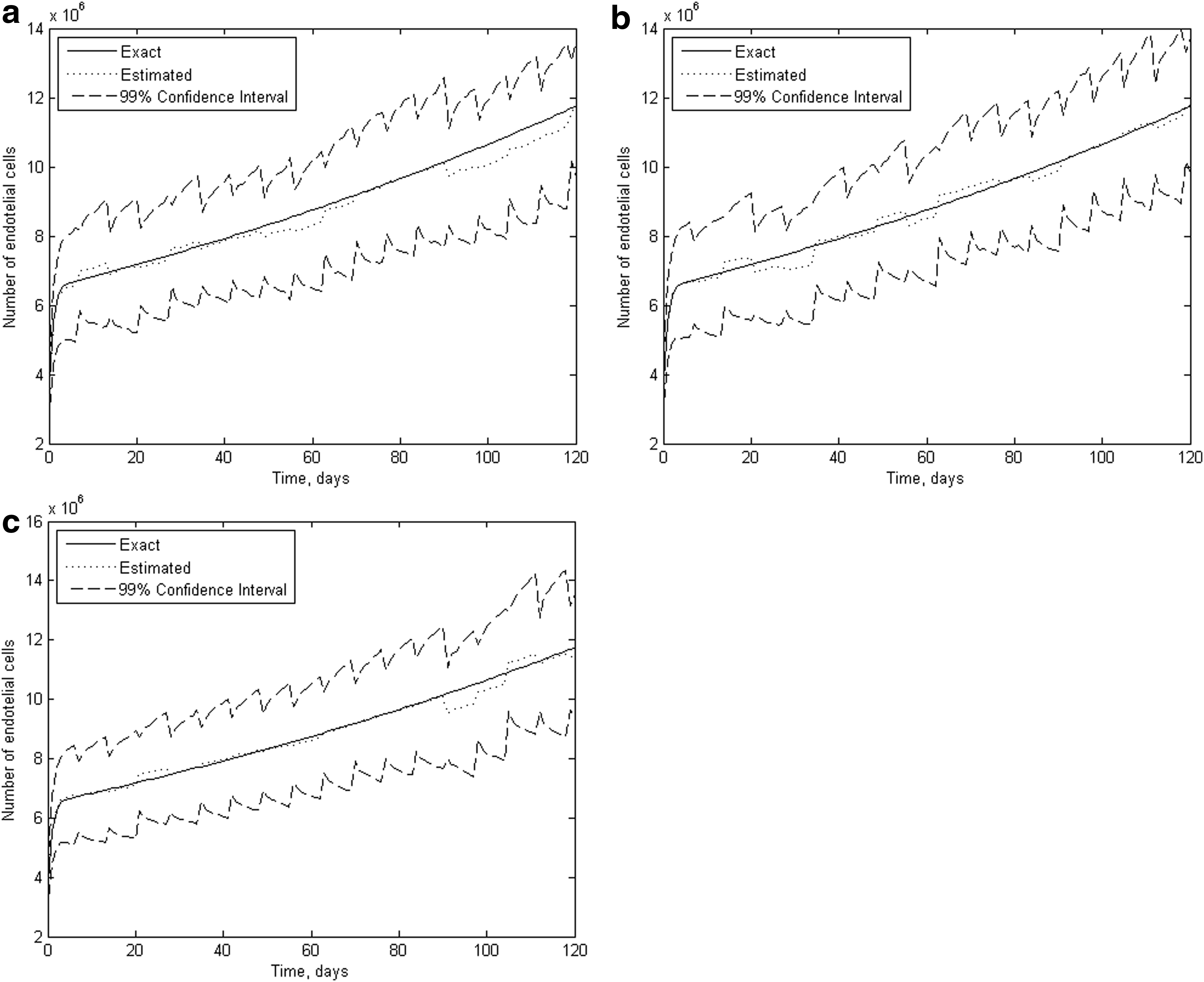
Figures 1 and 2 present the exact values and the results for the estimation of the numbers of tumor and endothelial cells, respectively, obtained with 500, 1000, and 2000 particles. Such state variables were chosen for this analysis because measurements are available for the number of tumor cells, but not for the number of endothelial cells. The behaviors presented in these figures are typical of those for the other state variables. The results are presented in the form of the means and of the 99% confidence bounds of each state variable, based on one single run of the particle filter. Figure 1 also presents the simulated measurements, which were taken every 7 days, as well as their 99% confidence bounds. Although the RMS errors basically decrease by increasing the number of particles (see Table 3), we note in Figures 1 and 2 that, in the graph scale, the results are very little affected by increasing the number of particles and estimated means tend to closely follow the exact values of the number of tumor cells, as well as the number of endothelial cells.

OPEN IN VIEWER

FIG. 1.

Estimation of the number of tumor cells for (a) 500 particles, (b) 1000 particles, and (c) 2000 particles.

OPEN IN VIEWER

FIG. 2.

Estimation of the number of endothelial cells for (a) 500 particles, (b) 1000 particles, and (c) 2000 particles.

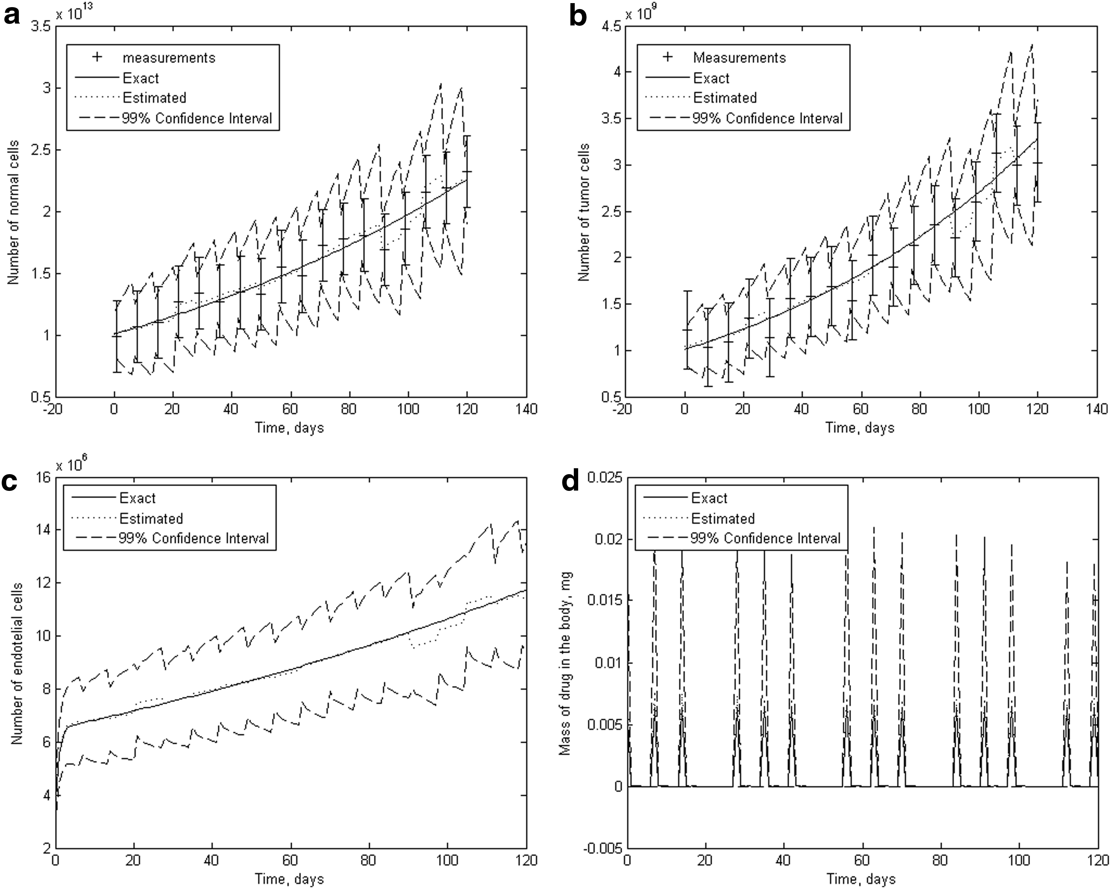
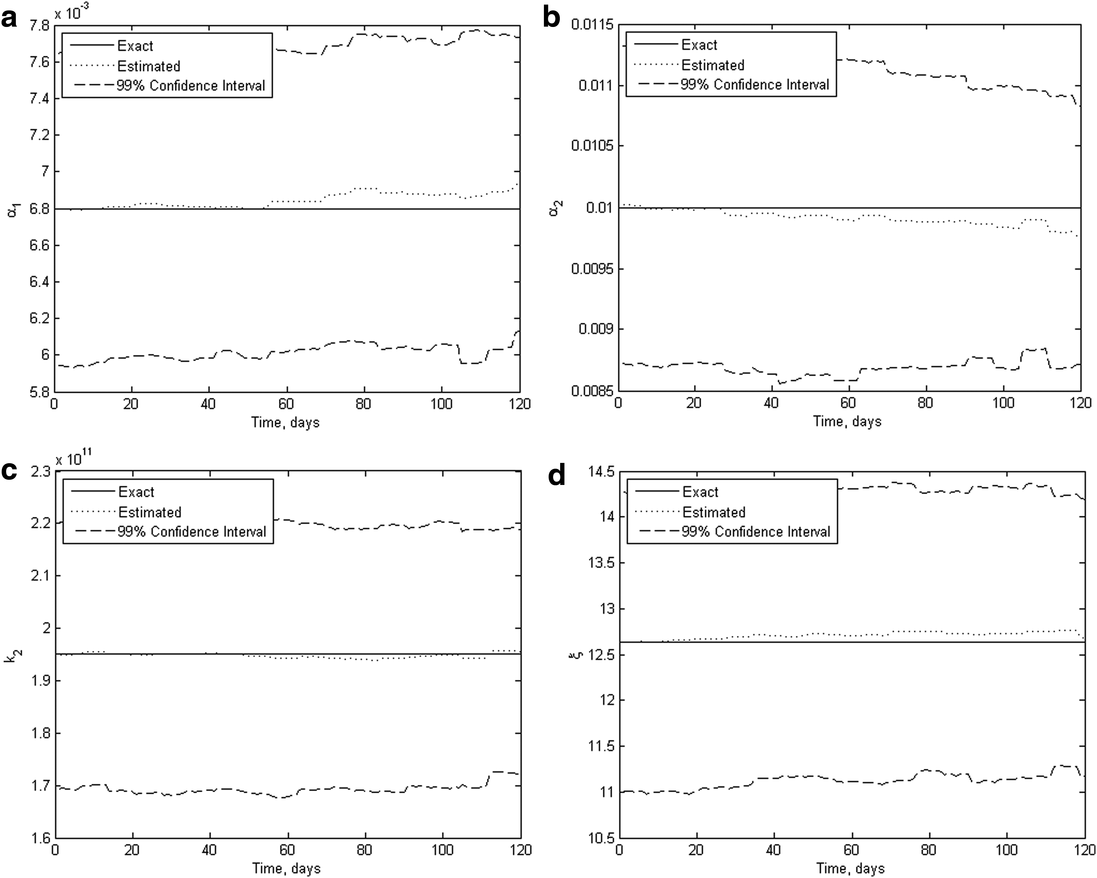
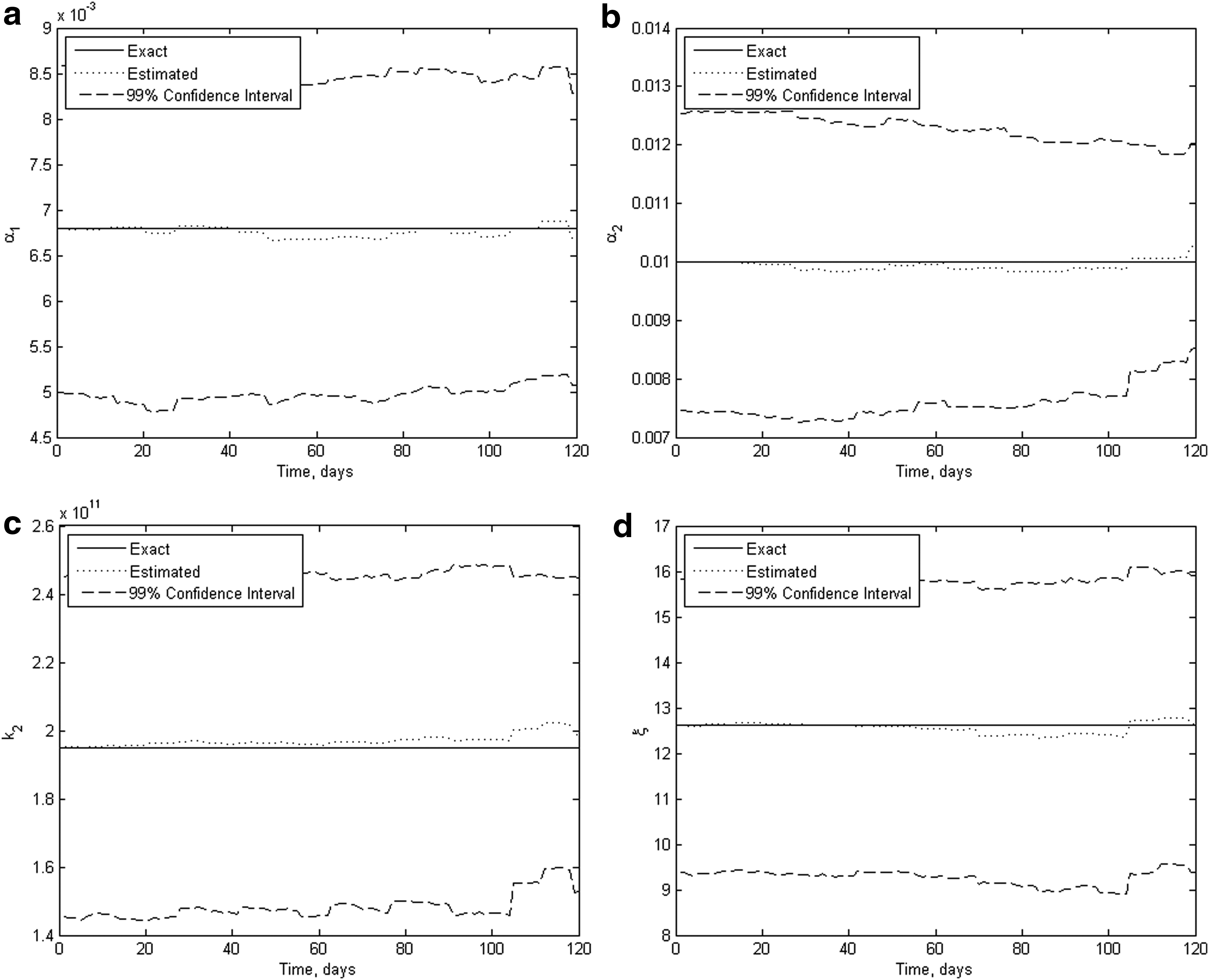
Figure 3 presents the estimations of the state variables, obtained with 2000 particles and standard deviations of 5% of the corresponding maximum values for the state evolution model, measurements, and model parameters. Similarly, the random behavior of selected model parameters, namely, α₁, α₂, k₂, and ξ, is presented in Figure 4. We note in Figure 3b and c that, with the proposed model and with the current model parameters, the numbers of tumor and endothelial cells increase despite the action of chemotherapy, in the time period selected for the analysis. The drug infusion in accordance with the protocol of one administration per week for three consecutive weeks, followed by one week of rest, is apparent in Figure 3d. Figure 3a–d shows that the estimated means are in excellent agreement with the exact values of the state variables. The 99% confidence bounds for the numbers of normal and tumor cells increase during the periods between measurements (see Fig. 3a,b). Such bounds for the number for endothelial cells and the mass of drug in the body (see Fig. 3c,d) relatively increase as time evolves, due to the lack of measurements of such variables. However, these variables are still quite accurately estimated by using only the measurements of tumor and normal cells. The model parameters show an excellent agreement with the exact ones, as illustrated by Figure 4a–d. Such behavior for α₁, α₂, k₂, and ξ is representative for the other parameters.

OPEN IN VIEWER

FIG. 3.

Estimation of state variables with 2000 particles and standard deviations of 5% for the state evolution model, measurements, and model parameters.

OPEN IN VIEWER

FIG. 4.

Estimation of selected model parameters with 2000 particles and standard deviations of 5% for the state evolution model, measurements, and model parameters.

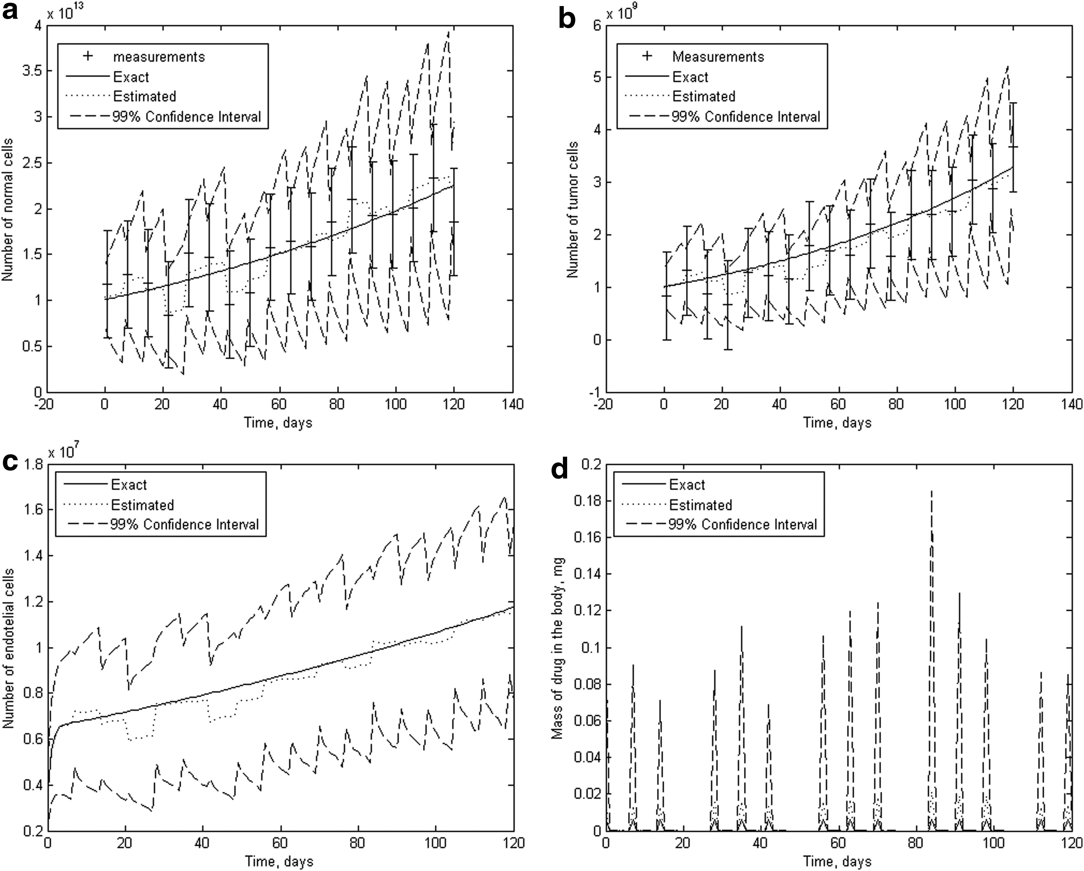
Results similar to those of Figures 3 and 4 are presented in Figures 5 and 6, for standard deviations of 10% of the corresponding maximum values for the state evolution model, measurements, and model parameters. Figures 5 and 6 show that excellent estimates are obtained for the means of state variables and parameters, even with such extremely large uncertainties in the evolution model, measurements, and model parameters. As expected, the 99% confidence intervals are wider than those for standard deviations of 5% (see Figs. 3 and 4), as a result of the larger uncertainties in the present case.

OPEN IN VIEWER

FIG. 5.

Estimation of state variables with 2000 particles and standard deviations of 10% for the state evolution model, measurements, and model parameters.

OPEN IN VIEWER

FIG. 6.

Estimation of selected model parameters with 2000 particles and standard deviations of 10% for the state evolution model, measurements, and model parameters.

5. Conclusions

This work dealt with the solution of a state estimation problem for the monitoring of tumor growth. The forward model was based on a system of nonlinear ordinary differential equations. The state estimation problem was solved by using simulated measurements of the numbers of tumor and normal cells. Uncertainties in the evolution model, measurements, and in the model parameters were taken into account in the solution procedure, which was based on the algorithm proposed by Liu and West that makes use of the ASIR particle filter. Such uncertainties were assumed as additive, Gaussian, with zero means and known covariance matrices.

Results obtained with uncertainties of standard deviations of 5% and 10% (of the maximum values of state variables, measurements, and model parameters) reveal that the present solution procedure is very accurate and robust. Even for such large values of standard deviations, the estimated means are in excellent agreement with the exact values of state variables and model parameters. The corresponding uncertainties of the estimated quantities could be appropriately identified by using an adequate number of particles in the solution approach. In addition, accurate results could be obtained within computational times of about 20 minutes by using only 500 particles.