Imbalanced Class Learning in Epigenetics

Abstract

In machine learning, one of the important criteria for higher classification accuracy is a balanced dataset. Datasets with a large ratio between minority and majority classes face hindrance in learning using any classifier. Datasets having a magnitude difference in number of instances between the target concept result in an imbalanced class distribution. Such datasets can range from biological data, sensor data, medical diagnostics, or any other domain where labeling any instances of the minority class can be time-consuming or costly or the data may not be easily available. The current study investigates a number of imbalanced class algorithms for solving the imbalanced class distribution present in epigenetic datasets. Epigenetic (DNA methylation) datasets inherently come with few differentially DNA methylated regions (DMR) and with a higher number of non-DMR sites. For this class imbalance problem, a number of algorithms are compared, including the TAN+AdaBoost algorithm. Experiments performed on four epigenetic datasets and several known datasets show that an imbalanced dataset can have similar accuracy as a regular learner on a balanced dataset.

1. Introduction

Currently, there is an explosion of data in a number of different scientific areas. New techniques are being developed every day to analyze, mine, annotate, and classify these data. After retrieval of data, a natural assumption is that if the dataset contains multiple classes, where each instance can be labeled as belonging to a particular class, then all classes have equal or almost the same number of instances. Once machine learning techniques are applied, the classifier tries to learn from the dataset with the assumption that the target concepts can be learned with equal weights from all instances. Unfortunately, this assumption does not always hold. Often there exists an unequal distribution among classes. Unequal distributions can range from a class being slightly larger or smaller than the other to extreme cases where the difference can be of several orders of magnitude larger, for example, the majority class is 100:1 or 1000:1 of the minority class. For example, in the case of detection of oil spills from satellite images, the authors had 41 positive examples against 896 negative examples, where the majority class consists of 96% of the data (Kubat et al., 1998). In these circumstances, the classifier learns most of the target concepts of the majority class and learns target concepts from the minority class poorly or not at all. So, once the learning is complete, when the classifier is applied to the test set the classifier seems to predict the majority class accurately while failing to predict the minority class at all. There also may be many instances in the majority class that are redundant, so the classifier learns from those instances more than learning from important instances in the minority class. Often the interest is more on the minority class such that getting rare instances from the minority class can be time-consuming and costly.

An unequal distribution between classes of a dataset is known as the class imbalance problem (Japkowicz and Holte, 2001; Chawla et al., 2004; Weiss, 2004; He and Garcia, 2009). This problem is prevalent in many domains such as in credit card fraud detection (Chan and Stolfo, 1998), network intrusion (Cieslak et al., 2006), text categorization (Dumais et al., 1998), and classification of proteins (Radivojac et al., 2004) to name a few. The importance of the imbalanced class problem has been more visible recently with the introduction of this topic in several conferences and journals. Recently, a few workshops have been held mainly addressing this area such as the Workshop on Class Imbalances: Past, Present, Future (CIPPF, 2012) and the International Conference on Machine Learning workshop on Learning from Imbalanced Data Sets (ICML, 03) among others.

The current study addresses the imbalanced class problem in epigenetics (Waddington, 1953; Weber and Schubeler, 2007; Bock and Lengauer, 2008). The epigenetic data sets were obtained from epigenetic transgenerational inheritance experiments (Guerrero-Bosagna et al., 2010, 2013; Bhandari et al., 2012a; Manikkam et al., 2012a,b,c, 2013; Nilsson et al., 2012; Tracey et al., 2013). The gestating female (F0 generation) exposed to environmental compounds had offspring that were bred out three generations to the F3 (great grand-offspring), and the sperm was collected from the males for analysis. The number of altered sites with differentially DNA methylated regions (DMR) was identified in a comparison of F3 generation male sperm from exposure lineage and control lineage F3 generations. For each study observing changes in DNA methylation between control and exposure lineages, there are only a few DMR sites compared with thousands of sites that are not altered (non-DMRs). Therefore, using machine learning methods in this scenario creates a problem of data imbalance. For many biological datasets (e.g., disease outbreaks), this class imbalance problem is inherent.

One of the main issues with epigenetic datasets is that they are naturally imbalanced. A number of steps in the analysis such as stringent statistics, intersection between results, and other methods are used to make sure that the epigenetic sites retrieved from the analysis contain as few false positives as possible. Only a few of these sites are later confirmed using alternate procedures such as bisulfite sequencing (Chen et al., 2005). Since such stringent analysis methods pick only a very limited number of epigenetic sites from the whole genome, the rest of the sites all fall in the majority class and the epigenetic sites fall in the minority class.

Another issue from the machine-learning point of view is that most biological datasets come with high dimension and low volume. Each site may contain from a few hundred to a few thousand genomic features ranging from repeat elements to CpG islands (Gardiner-Garden and Frommer, 1987) to other characteristics. Among the many features, the relevant and important features need to be identified and kept as features in the dataset. Some of the selection of these features comes from biological knowledge of the dataset.

Both random oversampling (Han et al., 2005; Chawla et al., 2011) and random undersampling (Holte et al., 1989; Mease et al., 2007) have been used widely to address the class imbalance problem. Since they introduce overfitting and potential loss of subconcepts, many variants of these techniques have been proposed and used successfully. Using a synthetic dataset to overcome the minority class distribution is a unique technique. It uses the feature space in the minority class and creates new instances. One successful technique is synthetic minority oversampling technique (SMOTE) (Chawla et al., 2011). Tomek links is a data cleaning technique that can be used to create distinct clusters in the training set by removing overlapping examples, which helps create better classification rules (Tomek, 1976). Cluster-based oversampling (CBO) algorithms such as the one that uses K-means clustering create well-defined cluster boundaries and cluster means (Jo and Japkowicz, 2004). Cost-sensitive approaches based on the cost matrix have been used. Three cost-sensitive boosting methods, AdaC1, AdaC2, and AdaC3 (Sun et al., 2007), have been used where different costs are added in the weight update phase of the boosting algorithm.

An undersampling method called EasyEnsemble (Liu et al., 2009) has been used in this study. It converts the majority class instances of the training set into a number of subsets and allows a single classifier (AdaBoost is used to train each classifier) to be trained from each of these subsets plus the minority set. An ensemble learning system combines the outcome of these classifiers to create the final output. The approach proposed in this article also uses subset sampling optimization (SSO) (Yang et al., 2009, 2011) and the AdaBoost+TAN learning technique. These algorithms will be used in the current study.

2. Methods

2.1. EasyEnsemble

EasyEnsemble groups majority class instances into equal subsets of the same size of the minority class. After adding the entire minority class samples to each of these majority class subgroups, it trains a different learner on each subgroup. EasyEnsemble uses an ensemble-based approach that combines the output of these learners.

Algorithm 1. EasyEnsemble
Input: P: minority class examples
N: majority class examples
T: number of subsets from the majority class examples
s_i: number of iterations for training AdaBoost ensemble H_i
Output: An ensemble of ensembles
\documentclass{aastex}\usepackage{amsbsy}\usepackage{amsfonts}\usepackage{amssymb}\usepackage{bm}\usepackage{mathrsfs}\usepackage{pifont}\usepackage{stmaryrd}\usepackage{textcomp}\usepackage{portland, xspace}\usepackage{amsmath, amsxtra}\pagestyle{empty}\DeclareMathSizes{10}{9}{7}{6}\begin{document} $${H (x)} = {\rm sgn} \left(\sum\limits_{i = 1}^T \sum \nolimits_{j = 1}^{s_i} \alpha_{i , j} h_{i , j} (x) - \sum \nolimits_{i = 1}^T \theta_i \right)$$ \end{document}
procedure: EasyEnsemble(P,N,T,s_i )
for i = 1 to T
Create N_i by randomly selecting a subset of examples from N, such that \|N_i \| = \|P\|
Train H_i from P+N_i. H_i consists of s_i weak classifiers h_i,j with weights α_i,j
This ensemble H_i has threshold θ_i
end for
end procedure

One of the characteristics of the EasyEnsemble algorithm is that it looks like an ensemble of ensembles. As shown in Algorithm 1, the majority class is divided into T balanced subsamples each containing the complete minority class P. In each iteration a classifier H_i is trained. Classification and regression trees (CART) (Breiman et al., 1984) are used as the base classifier in EasyEnsemble. H_i is actually an ensemble of s_i weak classifiers h_ij (CART) with weights α_i,j. A weak classifier is one that achieves accuracy better than random guessing. If h_i,j is assumed to be a set of features, then H_i is actually a linear classifier built on those features. So features in different subsets have information of different viewpoints of the majority class. Finally, all those features h_i,j ( \documentclass{aastex}\usepackage{amsbsy}\usepackage{amsfonts}\usepackage{amssymb}\usepackage{bm}\usepackage{mathrsfs}\usepackage{pifont}\usepackage{stmaryrd}\usepackage{textcomp}\usepackage{portland, xspace}\usepackage{amsmath, amsxtra}\pagestyle{empty}\DeclareMathSizes{10}{9}{7}{6}\begin{document} $$i = 1 , 2 , \ldots , T$$ \end{document} and \documentclass{aastex}\usepackage{amsbsy}\usepackage{amsfonts}\usepackage{amssymb}\usepackage{bm}\usepackage{mathrsfs}\usepackage{pifont}\usepackage{stmaryrd}\usepackage{textcomp}\usepackage{portland, xspace}\usepackage{amsmath, amsxtra}\pagestyle{empty}\DeclareMathSizes{10}{9}{7}{6}\begin{document} $$j = 1 , 2 , \ldots , s_i$$ \end{document} ) are used to create the final ensemble classifier. The range of values for threshold Θ used is from −∞ to +∞ and the value returned by the weak classifier directly. The value of Θ was chosen to get the entire range for the pairs (false position rate, true positive rate) to build the ROC curve from the data. The threshold (Θ) is computed by summing up all the weight update parameters from each iteration and dividing by 2. The final threshold for the ensemble is the sum of all T rounds of thresholds. For this article the number of subsets of negative examples used is T = 4, and the number of iterations to train AdaBoost classifier is s_i = 10. For each dataset there are 4 subsets that are sampled, and 10 weak learners are trained based on them; hence, the final classifier is based on 40 weak learners. Since the imbalance level of the datasets used is below 40%, the authors (in Liu et al., 2009) chose 40 as an ideal number of weak learners and showed that by not utilizing all of the majority class examples they can train their classifier faster while minimizing some of the negative effects (caused by using all the majority class examples). Their classifier is comparable with other well-known class-imbalanced methods. As EasyEnsemble uses boosting inside of each bag (in bagging), this combination (boosting reduces bias and bagging reduces variance) of boosting and bagging improves performance. Details of this algorithm are given in the article by Liu et al. (2009).

2.2. Subset sampling optimization

Subset sampling optimization (SSO) is based on the particle swarm optimization (PSO) hybrid system (Yang et al., 2009, 2011). The SSO algorithm divides the dataset into three sets. While the first two are used for internal cross validation to perform the internal optimization process, the third set is used for external cross validation. The internal dataset is again divided into three sets, two for training and the other for testing. Using the internal dataset the SSO algorithm takes different subset samples of the majority class and combines them with samples from the minority class for classifier learning (both sets are of equal size). Each of these sets is called a particle and has an index in the particle space. Each of these n particles also has a dimension m equal to the number of instances in it. A particle's velocity v_i_,j(t) (index \documentclass{aastex}\usepackage{amsbsy}\usepackage{amsfonts}\usepackage{amssymb}\usepackage{bm}\usepackage{mathrsfs}\usepackage{pifont}\usepackage{stmaryrd}\usepackage{textcomp}\usepackage{portland, xspace}\usepackage{amsmath, amsxtra}\pagestyle{empty}\DeclareMathSizes{10}{9}{7}{6}\begin{document} $$i = 1 , 2 , \ldots , n$$ \end{document} and \documentclass{aastex}\usepackage{amsbsy}\usepackage{amsfonts}\usepackage{amssymb}\usepackage{bm}\usepackage{mathrsfs}\usepackage{pifont}\usepackage{stmaryrd}\usepackage{textcomp}\usepackage{portland, xspace}\usepackage{amsmath, amsxtra}\pagestyle{empty}\DeclareMathSizes{10}{9}{7}{6}\begin{document} $$j = 1 , 2 , \ldots , m$$ \end{document} ) and position x_i,j(t) are updated using the binary particle swarm optimization (BPSO) (Kennedy and Eberhart, 1997; Lee et al., 2008) and the following equations. \documentclass{aastex}\usepackage{amsbsy}\usepackage{amsfonts}\usepackage{amssymb}\usepackage{bm}\usepackage{mathrsfs}\usepackage{pifont}\usepackage{stmaryrd}\usepackage{textcomp}\usepackage{portland, xspace}\usepackage{amsmath, amsxtra}\pagestyle{empty}\DeclareMathSizes{10}{9}{7}{6}\begin{document} \begin{align*}v_{i , j} (t + 1) = wv_{i , j} (t) + c_1R_1 (pbest_{i , j} - x_{i , j} (t)) + c_2R_2 (gbest_{i , j} - x_{i , j} (t)) \tag{1}\end{align*} \end{document} \documentclass{aastex}\usepackage{amsbsy}\usepackage{amsfonts}\usepackage{amssymb}\usepackage{bm}\usepackage{mathrsfs}\usepackage{pifont}\usepackage{stmaryrd}\usepackage{textcomp}\usepackage{portland, xspace}\usepackage{amsmath, amsxtra}\pagestyle{empty}\DeclareMathSizes{10}{9}{7}{6}\begin{document} \begin{align*}x_{i , j} (t + 1) = \begin{cases}0 , \ if.random () \geq s (v_{ij} (t + 1)) \\ 1 , \ if.random () < s (v_{i , j} (t + 1)) \end{cases} \tag{2}\end{align*} \end{document} \documentclass{aastex}\usepackage{amsbsy}\usepackage{amsfonts}\usepackage{amssymb}\usepackage{bm}\usepackage{mathrsfs}\usepackage{pifont}\usepackage{stmaryrd}\usepackage{textcomp}\usepackage{portland, xspace}\usepackage{amsmath, amsxtra}\pagestyle{empty}\DeclareMathSizes{10}{9}{7}{6}\begin{document} \begin{align*}S (v_ {i , j} (t + 1)) = \frac {1} {1 + e^ {- v_ {i , j} (t + 1)}} \tag {3} \end{align*} \end{document}

Here pbest_i,j and gbest_i,j are the previous best position and updated best position, w is the fitness weight, c₁, R₁, c₂, and R₂ are the learning rates and social coefficients, while function random provides pseudo-random numbers to create uniform distribution between 0 and 1. When the value x_i,j is 1, then the jth sample is included in building the classification model, while a value of 0 will have it excluded from the training. Among these subsets the ones that create better classification accuracy are favored and optimized in each iteration. The overall fitness of each particle (subset) is evaluated with the following function. \documentclass{aastex}\usepackage{amsbsy}\usepackage{amsfonts}\usepackage{amssymb}\usepackage{bm}\usepackage{mathrsfs}\usepackage{pifont}\usepackage{stmaryrd}\usepackage{textcomp}\usepackage{portland, xspace}\usepackage{amsmath, amsxtra}\pagestyle{empty}\DeclareMathSizes{10}{9}{7}{6}\begin{document} \begin{align*}\hbox {Overall fitness} (sample) = \sum \limits_ {i = 1} ^L \frac {w_1 \times AUC (sample) + w_2 \times FMeasure (sample) + w_3 \times Gmean (sample)} {L} \tag {4} \end{align*} \end{document}

L is the number of classifiers in the hybrid system (in the SSO algorithm five classifiers are used for the training; they are decision tree [J48], k-nearest neighbor [KNN], naive Bayes [NB], random forest [RF], and logistic regression [LOG]), and w₁, w₂, and w₃ are the fitness weights with equal values w₁ = w₂ = w₃ = 1/3 ( \documentclass{aastex}\usepackage{amsbsy}\usepackage{amsfonts}\usepackage{amssymb}\usepackage{bm}\usepackage{mathrsfs}\usepackage{pifont}\usepackage{stmaryrd}\usepackage{textcomp}\usepackage{portland, xspace}\usepackage{amsmath, amsxtra}\pagestyle{empty}\DeclareMathSizes{10}{9}{7}{6}\begin{document} $$\sum_{i = 1}^3 w_i = 1$$ \end{document} ). In each cross-validation fold all of the particles' position and velocity are initialized, and in each of T (150) iterations the particles' position and velocity are updated based on their overall fitness. After each fold the particles' information is saved. Once the training is completed, the subset from each iteration is taken and the majority class instances are ranked based on their classification accuracy from the SSO algorithm. These instances are combined with the minority class instances to construct a balanced dataset. The classifiers used for training are not the same classifiers used for evaluation, which produces an independent unbiased evaluation. Pseudocode for the algorithm is presented in Algorithm 2. Details of the algorithm are given in Yang et al. (2009) and Yang et al. (2011).

Algorithm 2. Subset Sampling Optimization (SSO)
Input: trainSet: majority and minority class examples
CrossValidationSize = = internalCrossVal(trainFold) //Size of internal cross validation for training
PopulationSize: number of particles // particle = (all examples of minority class)+(subset of majority class)
MajoritySize: dimension of the particle (samples in majority subclass)
T : number of iterations to update the particles' position and velocity
Output: A ranked list of the majority class examples
procedure: BPSO_Hybrid(trainSet,CrossValidationSize,PopulationSize,MajoritySize,T)
for I = 1 to CrossValidationSize do
for j = 1 to PopulationSize do
for k = 1 to MajoritySize do
initialize position and velocity of particle x_i,j (t) // allocate position/velocity of all particles
end for
end for
for t = 0 to T // iteration of T = 150 used
for each particle do
Update internal training set based on particle position
Train classifiers based on updated training set
Evaluate test set with trained classifier and calculate overall fitness value
Overall fitness (sample)= \documentclass{aastex}\usepackage{amsbsy}\usepackage{amsfonts}\usepackage{amssymb}\usepackage{bm}\usepackage{mathrsfs}\usepackage{pifont}\usepackage{stmaryrd}\usepackage{textcomp}\usepackage{portland, xspace}\usepackage{amsmath, amsxtra}\pagestyle{empty}\DeclareMathSizes{10}{9}{7}{6}\begin{document} $$\sum \nolimits_ {i = 1} ^L \frac {w_1 \times AUC (sample) + w_2 \times FMeasure (sample) + w_3 \times Gmean (sample)} {L} $$ \end{document}
Update v_ij(t) and x_i,j(t) // updated using Equations 1 –3
end for
end for
resultSet = resultSet ∪ save(particles) // saves these subsets with their classification accuracy
end for
finalmajorityclass = rank(resultSet) // rank subsets based on their classification accuracy by SSO

2.3. TAN-based AdaBoost

This method uses the tree augmented Bayesian network (TAN) as a base classifier for the AdaBoost algorithm, so this algorithm is called TAN+AdaBoost. First, the advantages of using TAN (Friedman et al., 1997) over regular naive Bayes classifier (NBC) need to be explained.

Regular naive Bayes assumes conditional independence among different attributes. Figure 1a shows a simple network where each feature is pointed to by the parent class node and each attribute can be only a child node. The joint probability can be calculated through the class probabilities multiplied by the class conditional probability

FIG. 1.

The naive Bayes assumes conditional independence among different attributes. 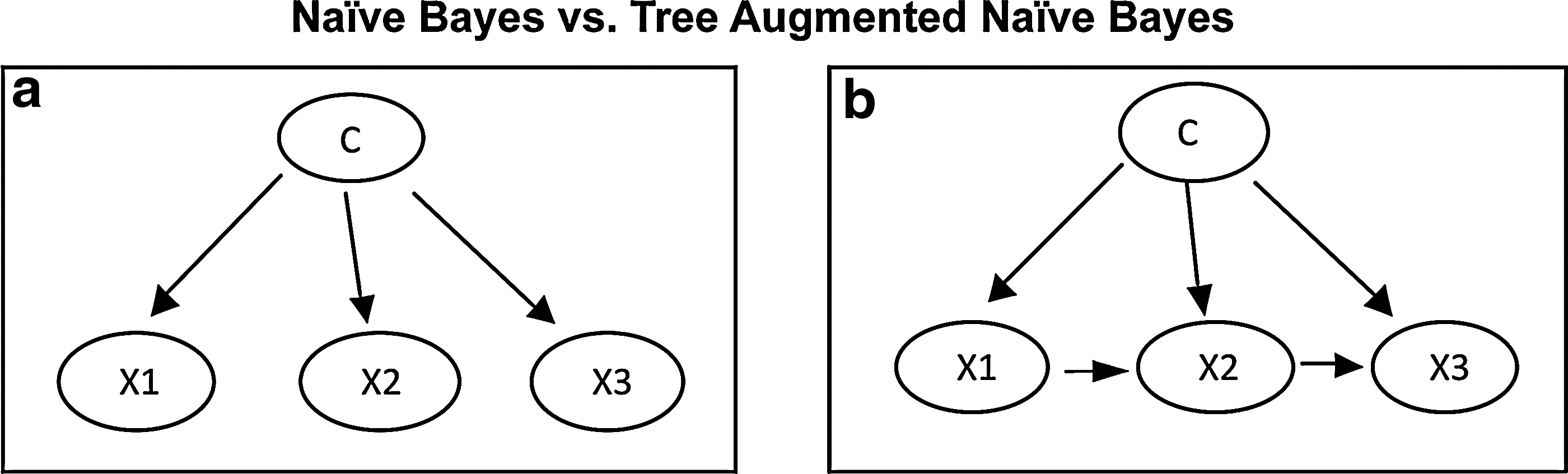(a) The parent node points to each of the child nodes. (b) A tree augmented naive Bayes has an additional augmented edge from a child node to its sibling, which is based on statistical dependencies.

\documentclass{aastex}\usepackage{amsbsy}\usepackage{amsfonts}\usepackage{amssymb}\usepackage{bm}\usepackage{mathrsfs}\usepackage{pifont}\usepackage{stmaryrd}\usepackage{textcomp}\usepackage{portland, xspace}\usepackage{amsmath, amsxtra}\pagestyle{empty}\DeclareMathSizes{10}{9}{7}{6}\begin{document} \begin{align*}p (c , x_1 , x_2 , \ldots , x_n) = p (c) \prod_{i}p (x_i \mid c)\end{align*} \end{document}

A tree-augmented naive Bayes classifier (TAN) augments the standard NBC by allowing each attribute to have an additional incoming edge (Fig. 1b). This augmented edge is created by statistical dependencies that show the correlation among the features. The TAN outperforms naive Bayes while maintaining computational simplicity by avoiding double accounting, which is present in naive Bayes where multiple features are used that have a high correlation value. The TAN model can be created as follows (Hong-Bo et al., 2002).

1. Compute the conditional mutual information (CMI) between each pair of features, \documentclass{aastex}\usepackage{amsbsy}\usepackage{amsfonts}\usepackage{amssymb}\usepackage{bm}\usepackage{mathrsfs}\usepackage{pifont}\usepackage{stmaryrd}\usepackage{textcomp}\usepackage{portland, xspace}\usepackage{amsmath, amsxtra}\pagestyle{empty}\DeclareMathSizes{10}{9}{7}{6}\begin{document} $$CMI (X , Y \mid C) = \sum_ {x , y , c} p (x , y , c) \log \frac {p (x , y \mid c)} {p (x \mid c) p (y \mid c)} $$ \end{document}

where C represents the class variable and \documentclass{aastex}\usepackage{amsbsy}\usepackage{amsfonts}\usepackage{amssymb}\usepackage{bm}\usepackage{mathrsfs}\usepackage{pifont}\usepackage{stmaryrd}\usepackage{textcomp}\usepackage{portland, xspace}\usepackage{amsmath, amsxtra}\pagestyle{empty}\DeclareMathSizes{10}{9}{7}{6}\begin{document} $$\{X_1 , \ldots , X_n \} $$ \end{document} are the features.

2. A complete undirected graph is created where the nodes represent the features. Each edge label represents the value of the CMI between the features.

3. Construct a maximum weighted spanning tree [e.g., Kruskal's algorithm (Kruskal, 1956)] from the graph.

4. Pick any arbitrary node as the root and have all the edges be outward from this root node. This creates a directed tree T out of an undirected tree.

5. Construct the TAN model by adding a vertex labeled by C (class) and having an arc from C to each variable x_i.

6. So what we have is the TAN model, which is the NB model augmented by edges in T.

7. Now calculate joint probability, which depends upon the conditional probability not only on the class but also on the feature's parent node parent_x. \documentclass{aastex}\usepackage{amsbsy}\usepackage{amsfonts}\usepackage{amssymb}\usepackage{bm}\usepackage{mathrsfs}\usepackage{pifont}\usepackage{stmaryrd}\usepackage{textcomp}\usepackage{portland, xspace}\usepackage{amsmath, amsxtra}\pagestyle{empty}\DeclareMathSizes{10}{9}{7}{6}\begin{document} $$p (c , x_1 , x_2 , \ldots , x_n) = p (c) \prod_{i = 1}^n p (x_i \mid parent_{x_i} , c)$$ \end{document}

TAN is used as the base classifier for the AdaBoost algorithm. The details of the TAN+AdaBoost algorithm are given in Algorithm 3.

Algorithm 3. TAN+AdaBoost
Input: An imbalanced dataset
\documentclass{aastex}\usepackage{amsbsy}\usepackage{amsfonts}\usepackage{amssymb}\usepackage{bm}\usepackage{mathrsfs}\usepackage{pifont}\usepackage{stmaryrd}\usepackage{textcomp}\usepackage{portland, xspace}\usepackage{amsmath, amsxtra}\pagestyle{empty}\DeclareMathSizes{10}{9}{7}{6}\begin{document} $$(x_1 , y_1) , \ldots , (x_m , y_m) ,$$ \end{document} , where x_i in X, y_i in Y = {−1, +1}
Output: The final classifier
procedure: TAN+AdaBoost
Initialize D₁(i) = 1/m
while (t < T) do: // committee of T classifiers (T = 10)
1. Train the base learner (TAN) using distribution D_t resulting in classifier h_t
2. Select a weight update parameter : \documentclass{aastex}\usepackage{amsbsy}\usepackage{amsfonts}\usepackage{amssymb}\usepackage{bm}\usepackage{mathrsfs}\usepackage{pifont}\usepackage{stmaryrd}\usepackage{textcomp}\usepackage{portland, xspace}\usepackage{amsmath, amsxtra}\pagestyle{empty}\DeclareMathSizes{10}{9}{7}{6}\begin{document} $$\alpha_t = \frac {1} {2} \ln \left(\frac {1 - \varepsilon_t} {\varepsilon_t} \right)$$ \end{document}
where \documentclass{aastex}\usepackage{amsbsy}\usepackage{amsfonts}\usepackage{amssymb}\usepackage{bm}\usepackage{mathrsfs}\usepackage{pifont}\usepackage{stmaryrd}\usepackage{textcomp}\usepackage{portland, xspace}\usepackage{amsmath, amsxtra}\pagestyle{empty}\DeclareMathSizes{10}{9}{7}{6}\begin{document} $$\varepsilon_t = \frac {w_e} {w} $$ \end{document} , the error rate given the weights of the data points (total weight of all data points w = w_c +w_e) and \documentclass{aastex}\usepackage{amsbsy}\usepackage{amsfonts}\usepackage{amssymb}\usepackage{bm}\usepackage{mathrsfs}\usepackage{pifont}\usepackage{stmaryrd}\usepackage{textcomp}\usepackage{portland, xspace}\usepackage{amsmath, amsxtra}\pagestyle{empty}\DeclareMathSizes{10}{9}{7}{6}\begin{document} $$w_e = \sum_{y_i \neq h_t}x_i$$ \end{document} at iteration t.
3. Update
\documentclass{aastex}\usepackage{amsbsy}\usepackage{amsfonts}\usepackage{amssymb}\usepackage{bm}\usepackage{mathrsfs}\usepackage{pifont}\usepackage{stmaryrd}\usepackage{textcomp}\usepackage{portland, xspace}\usepackage{amsmath, amsxtra}\pagestyle{empty}\DeclareMathSizes{10}{9}{7}{6}\begin{document} $$D_ {t + 1} (i) = \frac {D_t (i)} {Z_t} \times \begin{cases} e^ {- \alpha_t} , \ {if} ..h_t (x_i) = y_i \\ e^ {\alpha_t} , \ {if} ..h_t (x_i) \neq y_i \end{cases}$$ \end{document}
= D_t(i)exp(−α_th_t (x_i)y_i)/Z_t
where Z_t is the normalization factor so that D_t₊₁ is a distribution
end while
return \documentclass{aastex}\usepackage{amsbsy}\usepackage{amsfonts}\usepackage{amssymb}\usepackage{bm}\usepackage{mathrsfs}\usepackage{pifont}\usepackage{stmaryrd}\usepackage{textcomp}\usepackage{portland, xspace}\usepackage{amsmath, amsxtra}\pagestyle{empty}\DeclareMathSizes{10}{9}{7}{6}\begin{document} $$H (x) = {\rm sign} \left(\sum\limits_{t = 1}^T \alpha_t h_t (x) \right)$$ \end{document}
end procedure

AdaBoost is based on the boosting approach and is named as one of the top 10 data-mining algorithms (Wu et al., 2008). In AdaBoost, initially, all instances are given an equal weight. All the classifiers are trained with the same number of instances. After each iteration AdaBoost increases the weight of the incorrectly classified instances while decreasing the weight of the correctly classified instances. The goal is to try to correctly label the more difficult instances that the classifier labeled incorrectly. At the same time, each classifier is also assigned a weight based on its classification accuracy. This weight is used in the test phase, where more accurate classifiers get more confidence. When testing a new instance, each classifier gives a weighted vote, and the final label of the instance is based on the majority vote. Schapire proved that any weak classifier can be converted into a strong classifier by following the probably approximately corrected (PAC) learning framework (Freund and Schapire, 1996, 1997). A weak learner is one that achieves accuracy better than random guessing. Although TAN is considered better than NBC, we still consider TAN as a weak classifier and use it as the base classifier for AdaBoost. We name our approach TAN+AdaBoost.

2.4. Data sets

A total of nine different datasets were used in the experiments, all with 10-fold cross-validation. These datasets are from diverse domains. Five are taken from the University of California Irvine (UCI) repository (Bache and Lichman, 2013) and four are from the Skinner laboratory at Washington State University. The epigenetics datasets are from epigenetic transgenerational inheritance experiments and F3 generation somatic cells or sperm from various exposure lineages, including (i) Sertoli and granulosa somatic cells (Nilsson et al., 2012; Guerrero-Bosagna et al., 2013), (iii) dioxin (Hip), jet fuel (Jip), and vinclozolin (Vip) (Guerrero-Bosagna et al., 2010; Manikkam et al., 2012a, c; Tracey et al., 2013), and (iv) plastics (Bip) and pesticide (Pip) (Manikkam et al., 2012b, 2013). Another data set, (ii) Sox9-Sry-Tcf21 (Bhandari et al., 2012a,b), will be used as a negative control for the epigenetic datasets and is a transcription factor binding data set, but was obtained with similar technology. The Sertoli and granulosa datasets consist of adult vinclozolin lineage F3 generation somatic cells that influence the onset of testis and ovarian disease, respectively. The dioxin, jet fuel, and vinclozolin datasets consist of ancestral environmental exposures of these three compounds individually and are associated with the epigenetic transgenerational inheritance of adult onset diseases. Similarly, the plastics and pesticide datasets consist of ancestral environmental exposures of these compounds and are associated with the epigenetic transgenerational inheritance of adult onset diseases. The Sox9, Sry, and Tcf21 are transcription factors involved in the induction of Sertoli cell differentiation and testis development and the datasets are the specific transcription factor binding sites for these factors, so are not epigenetic data and are used as a negative control dataset. Among these datasets the epigenetic datasets (as well as the negative control dataset) are naturally imbalanced. However, the UCI datasets have been modified to create imbalance datasets by labeling one of the smaller classes as the minority class and the rest of the classes as the majority class. Details of these datasets are given in Tables 1 and 2. Table 1 shows the dataset name, features, total instances, number of features, and the percentage of the minority class to the total class distribution. Table 3 shows the general description of the datasets and also shows the target class.

Table 1.

Description of Selected Datasets

Dataset name	Type of features	Total instances	Number of features	% Minority class
Sertoli-granulosa	Numeric	1842	75	28.39
Sox9 Sry Tcf21	Numeric	5001	75	23.47
Dioxin, jet fuel, vinclozolin	Numeric	2446	52	30.08
Plastics, pesticide	Numeric	3879	74	16.94
Abalone	Numeric/nominal	4177	8	6.2
Letter	Numeric	20,000	17	3.79
Car	Numeric/nominal	1728	6	3.99
Balance	Numeric	625	4	7.84
Vehicle	Numeric	946	18	25.05

The table contains dataset names, types of features, total instances, number of features, and the total percentage of the minority class of the entire dataset.

Table 2.

Description of the University of California Irvine and Epigenetics Dataset

Dataset name	Description
Sertoli-granulosa	Adult somatic cell (Sertoli cell) that influences the onset of a specific disease (male infertility)
Sox9 Sry Tcf21	Induction of Sertoli cell differentiation and testis development
Dioxin, jet fuel, vinclozolin	Ancestral environmental exposures (3 compounds) associated with adult onset disease
Plastics, pesticide	Ancestral environmental exposures (2 compounds) associated with adult onset disease
Abalone	Age prediction of abalone from physical measures (number of rings)
Letter	Classify English alphabet based on image characteristics (fonts)
Car	Car acceptability evaluation based on price, comfort, etc.
Balance	Balance scale L,R,B based on weight and distance
Vehicle	Classify a given silhouette as one of the vehicles

Table contains the name and short description of each dataset.

Table 3.

The Area Under the Curve Scores from the Experiments

	Sertoli-granulosa	Sox9-Sry-Tcf21	Hip-Jip-Vip	Bip-Pip	Abalone	Letter	Car	Balance	Vehicle
	DMR	DMR	DMR	DMR	Class 6	Find R	Class good	Class B	Opel
Objective
Initial min	523	1173	736	101	259	758	69	49	212
Initial maj	1319	3828	1710	495	3918	19242	1659	576	634
Unbalanced
SMO	0.8138	0.5	0.935	0.884	0.5	0.604	0.5	0.5	0.5
Logistic	0.9647	0.852	0.999	0.968	0.897	0.942	0.975	0.414	0.857
J48	0.9399	0.775	1	0.999	0.498	0.928	0.975	0.489	0.768
RandomForest	0.9477	0.88	0.999	0.999	0.831	0.99	0.988	0.397	0.84
AdaBoost	0.9677	0.847	1	1	0.872	0.948	0.959	0.217	0.758
EasyEnsemble
Initial min	523	1173	736	101	259	758	69	49	212
Initial maj	1319	3828	1710	495	3918	19242	1659	576	634
AUC	0.9755	0.8416	0.866	0.9835	0.9113	0.9964	0.7692	0.4878	0.8295
Using SSO
Reduced min	523	1173	736	101	259	758	69	49	212
Reduced maj	523	1173	736	101	259	758	69	49	212
SSO+SMO	0.8432	0.845	0.947	0.906	0.873	0.972	0.877	0.296	0.762
SSO+Logistic	0.9565	0.959	0.999	0.95	0.939	0.996	0.949	0.198	0.898
SSO+J48	0.9379	0.937	0.999	0.995	0.884	0.987	0.964	0.54	0.821
SSO+RandomForest	0.9445	0.94	0.999	0.997	0.943	0.999	0.999	0.697	0.909
SSO+AdaBoost	0.9626	0.955	1	0.995	0.918	0.996	0.902	0.409	0.789
TAN+AdaBoost	0.965	0.812	0.997	0.998	0.874	0.993	0.973	0.489	0.774

Table contains the minority–majority class for each dataset (nine in total). The AUC values of the different classifiers applied to these datasets. SSO first balanced the dataset to equal class examples and then the same classifiers are applied as unbalanced dataset to calculate the AUC values. The last row contains the AUC values of TAN+AdaBoost approach on all datasets. AUC, area under the curve; SSO, subset sampling optimization. Bold indicates best classifier(s).

Genomic feature extraction (data collection) mining of epigenetic profiles starts with extraction of interesting properties from the DNA sequence data near DMR. After retrieving the training set, often the DMR locations are annotated to find the nearest gene name and the orientation of the gene. FASTA files are created from upstream and downstream of the target genes up to 100 kb. After construction of FASTA files for extraction of genomic features, tools such as RepeatMasker (Smit et al., 1996–2010) are used to find SINE, LINE, ERVL, ERV, and other repeat elements to the upstream and downstream of the DMR locations. One of the common ways of extracting genomic features from sequences is through identification of repeat elements. Identifying repeat elements and consensus sites helps to detect interesting patterns from these sites. Other genomic features are GC content (% of G [guanine] and C [cytosine] in the sequence) and CpG sites and density. Tools such as CpGislandSearcher (Takai and Jones, 2003) can be used to find CpG islands in these regions. CpG islands denote high frequency of CpG sites. A CpG site is denoted by a C followed immediately by a G. Epigenetic sites have been found in low CpG density regions, and therefore identification of a decrease in CpG density in interesting sites will be helpful.

Another important genomic feature is DNA sequence motifs (Stormo, 2000; Das and Dai, 2007). Common patterns among biologically relevant sites can be identified using motif findings. Motifs are DNA sequences that come with a probability matrix for each base position such that a certain combination of those sequences matches with every subsequence. These motifs are usually constructed by running DMR sites from related experiments through some of the popular motif-finding tools. The amount of genomic features can be enormous, and finding relevant genomic features that help to identify DMR sites is a challenge. For the murine imprinted gene project, the authors initially looked into 4 million genomic features (Luedi et al., 2005). Most of these features were constructed by combining different variations of features, ranking them based on which are more relevant, and then picking 4,000 of the most statistically significant ones for the final analysis (Luedi et al., 2005). For this study several motif-finding algorithms were used in order to discover motif sites and consensus sequence binding sites in the DMR regions that were used as important features in the extracted datasets.

3. Results

The three algorithms (EasyEnsemble, SSO, and TAN+AdaBoost) were applied on the nine imbalanced datasets. Among them, three are epigenetic datasets (Guerrero-Bosagna et al., 2010, 2013; Manikkam et al., 2012a,b,c, 2013; Nilsson et al., 2012; Tracey et al., 2013), one dataset (nonepigenetic) for specific DNA sequence binding site for Sry and Sox9 (Bhandari et al., 2012a,b), and five others are UCI datasets (Bache and Lichman, 2013).

The nine datasets were run using five popular nonimbalanced classifiers: (1) SVM, (2) logistic, (3) decision tree, (4) RandomForest, and (5) AdaBoost. Then, the nine datasets were run using the three imbalanced classifiers: (1) EasyEnsemble, (2) SSO, and (3) AdaBoost+TAN. For all algorithms, classifier accuracy measurements were done using area under the curve (AUC), F-measure, and G-mean. These results are given in Table 4 (AUC), Table 5 (F-measure), and Table 6 (G-mean).

Table 4.

The F-Measure Score

	Sertoli-granulosa	Sox9-Sry-Tcf21	Hip-Jip-Vip	Bip-Pip	Abalone	Letter	Car	Balance	Vehicle
Unbalanced
SMO	0.931	0.867	0.972	0.975	0.968	0.984	0.98	0.959	0.857
Logistic	0.956	0.857	0.992	0.977	0.968	0.985	0.979	0.959	0.865
J48	0.97	0.881	1	0.999	0.968	0.994	0.992	0.959	0.858
RandomForest	0.952	0.89	0.989	0.99	0.962	0.996	0.993	0.948	0.867
AdaBoost	0.972	0.867	1	1	0.968	0.982	0.98	0.959	0.858
EasyEnsemble	0.8354	0.7094	0.6519	0.8889	0.3712	0.6329	0.053	0.1176	0.5931
SSO
SSO+SMO	0.854	0.853	0.946	0.902	0.867	0.343	0.86	0.343	0.753
SSO+Logistic	0.891	0.884	0.981	0.869	0.873	0.237	0.902	0.237	0.828
SSO+J48	0.927	0.931	0.999	0.995	0.865	0.618	0.962	0.618	0.788
SSO+RandomForest	0.904	0.907	0.984	0.975	0.849	0.611	0.955	0.611	0.828
SSO+AdaBoost	0.928	0.933	1	0.995	0.869	0.408	0.922	0.408	0.749
TAN+AdaBoost	0.972	0.875	0.99	0.993	0.874	0.994	0.975	0.959	0.856

Table contains F-measure values from the algorithms applied to the nine datasets. Bold indicates best classifier(s).

Table 5.

The G-Mean Score

	Sertoli-granulosa	Sox9-Sry-Tcf21	Hip-Jip-Vip	Bip-Pip	Abalone	Letter	Car	Balance	Vehicle
Unbalanced
SMO	0.7925	0	0.9325943	0.8770159	0	0.4577	0	0	0
Logistic	0.9073	0.576348	0.9869621	0.9324628	0	0.6071	0.4935	0	0.6501
J48	0.9399	0.7371003	1	0.9989894	0	0.8994	0.9277	0	0.6806
RandomForest	0.8804	0.6767352	0.979014	0.9576386	0.3741	0.898	0.8822	0	0.5974
AdaBoost	0.9255	0	1	1	0	0.3306	0	0	0.3928
EasyEnsemble	0.8697	0.8312	0.7972	0.9706	0.8635	0.9748	0.3845	0.4619	0.7312
SSO
SSO+SMO	0.8397	0.8433	0.94687	0.90484	0.8717	0.2872	0.8681	0.2872	0.761
SSO+Logistic	0.89	0.88331	0.98097	0.8710621	0.876	0.2707	0.9051	0.2707	0.8278
SSO+J48	0.9263	0.93116	0.99932	0.99509	0.8667	0.4536	0.9631	0.4536	0.7942
SSO+RandomForest	0.8967	0.89976	0.98437	0.9751344	0.8494	0.5622	0.9555	0.5622	0.8227
SSO+AdaBoost	0.9229	0.92553	1	0.9950372	0.8706	0.4082	0.9247	0.4082	0.7617
TAN+AdaBoost	0.9309	0.7024798	0.981984	0.9929	0.3926	0.9057	0.5587	0	0.4285

Table contains G-measure values from the algorithms applied to the nine datasets. Bold indicates best classifier(s).

Table 6.

Combined Average

	Sertoli-granulosa	Sox9-Sry-Tcf21	Hip-Jip-Vip	Bip-Pip	Abalone	Letter	Car	Balance	Vehicle	Combined average (3 epigenetic datasets)	Combined average (5 UCI datasets)	Combined average (all 9 datasets)
SMO	0.8458	0.4557	0.9465	0.9120	0.4893	0.6819	0.4933	0.4863	0.4523	0.9014	0.5206	0.6404
Logistic	0.9427	0.7618	0.9927	0.9592	0.6217	0.8447	0.8158	0.4577	0.7907	0.9648	0.6134	0.7985
J48	0.9499	0.7977	1.0000	0.9990	0.4887	0.9405	0.9649	0.4827	0.7689	0.9830	0.7176	0.8214
RandomForest	0.9267	0.8156	0.9890	0.9822	0.7224	0.9613	0.9544	0.4483	0.7681	0.9660	0.7500	0.8409
AdaBoost	0.9551	0.5713	1.0000	1.0000	0.6133	0.7535	0.6463	0.3920	0.6696	0.9850	0.6929	0.7335
EasyEnsemble	0.8935	0.7941	0.7717	0.9477	0.7153	0.8680	0.4023	0.3558	0.7179	0.8710	0.6134	0.7185
SSO+SMO	0.8456	0.8471	0.9466	0.9043	0.8706	0.5341	0.8684	0.3087	0.7587	0.8988	0.6400	0.7649
SSO+Logistic	0.9125	0.9088	0.9870	0.8967	0.8960	0.5012	0.9187	0.2352	0.8513	0.9321	0.6743	0.7897
SSO+J48	0.9304	0.9331	0.9991	0.9950	0.8719	0.6862	0.9630	0.5372	0.8011	0.9748	0.7262	0.8574
SSO+RandomForest	0.9151	0.9156	0.9891	0.9824	0.8805	0.7241	0.9698	0.6234	0.8532	0.9622	0.7910	0.8726
SSO+AdaBoost	0.9378	0.9378	1.0000	0.9950	0.8859	0.6041	0.9162	0.4084	0.7666	0.9776	0.7632	0.8280
TAN+AdaBoost	0.9560	0.8032	0.9897	0.9946	0.7135	0.9642	0.8356	0.4827	0.6862	0.9801	0.7263	0.8251

Table contains average of the three values, AUC (Table 3), F-measure (Table 4), and G-mean (Table 5), after each algorithm applied to the nine datasets. By taking average of the three values, an unbiased result can be calculated. Bold indicates best classifiers.

For all datasets, 10-fold cross-validation was used to evaluate each of the three imbalanced class algorithms, EasyEnsemble, SSO, and TAN+AdaBoost. The SSO algorithm converts the data into a balanced distribution by selecting some examples from the majority class while keeping the minority class examples intact. This converted dataset was again input to the same five classifiers (SMO, Logistic, J48, RandomForest, and AdaBoost) using 10-fold cross-validation, and the results are given in the tables. Figures 2, 3, and 4 are barplots created from Tables 3, 4, and 5 for better visualization.

FIG. 2.

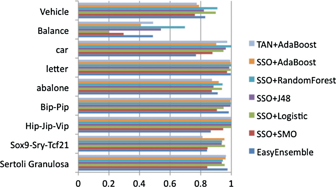
The AUC scores (from Table 3) of three imbalanced class learners (TAN+AdaBoost, SSO, and EasyEnsemble) on the nine datasets. The x-axis is the calculated AUC score. AUC, area under the curve; SSO, subset sampling optimization.

FIG. 3.

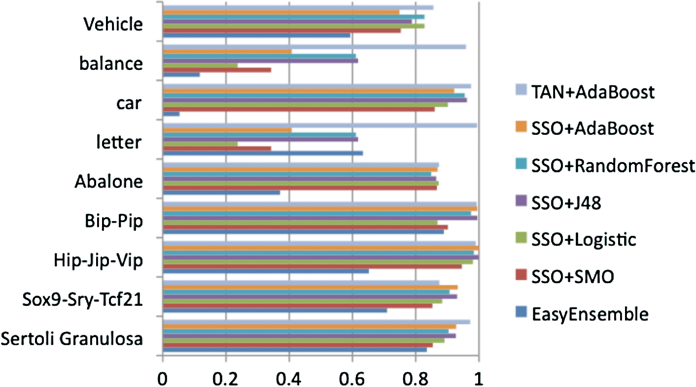
The F-measure (from Table 4) of three imbalanced class learners on nine datasets (x-axis is the F-measure score).

FIG. 4.

The G-mean (from Table 5) of three imbalanced class learners on nine datasets (x-axis is the G-mean score).

From Table 3, comparing AUC values across the four experiments, the AUC value improves for subset sampling optimization after SSO has converted the imbalanced distribution to a balanced class distribution. However, overall EasyEnsemble has a better AUC value on the four UCI datasets, while TAN+AdaBoost has better AUC values on the epigenetic datasets. The bold entry shows the best result obtained by a classifier for that particular dataset. The F-measure has decreased after having used SSO on the imbalanced dataset (Table 4). Considering F-measure, EasyEnsemble performs poorly on the five UCI datasets (Fig. 3). TAN+AdaBoost has a better F-measure on the epigenetic datasets. Comparing the G-mean score in Table 5, SSO again improves over imbalanced class distribution and closely matches EasyEnsemble on G-mean scores. The G-mean is zero for many of the unbalanced classes, because the classifier predicts only the majority class correctly while predicting all the minority class incorrectly. This shows the power of imbalanced class learning over nonimbalanced. This also justifies the need for using the proper evaluation method. On the three epigenetic datasets, Sertoli-granulosa, Hip-Jip-Vip, and Bip-Pip, TAN+AdaBoost had a higher AUC, F-measure, and G-mean than the rest of the algorithms. While on the negative-control dataset Sox9-Sry-Tcf21, TAN+AdaBoost underperforms in comparison with the others. The reason is that a biologically and molecularly different dataset is used for Sertoli cell transcription factor–binding sites (Bhandari et al., 2012a,b), and its motif and consensus binding sites differ from DMR sites. The datasets (Sertoli-granulosa, Hip-Jip-Vip, and Bip-Pip) consist of DMR sites that have differential DNA methylation changes between the F3 generation treatment and control lineages cells. These epigenetic data come from investigations of the actions of environmental factors during fetal development that induce epigenetic change in the germ line and promote epigenetic transgenerational inheritance of adult-onset diseases (Skinner et al., 2010). The other dataset (Sox9-Sry-Tcf21) consists of genome-wide transcription factor–binding sites in fetal Sertoli cells for Sry and Sox9. The Sox9-Sry-Tcf21 dataset includes identification of direct binding targets using a modified Chip–Chip comparative hybridization analysis (Bhandari et al., 2012a,b) and so is not an epigenetic dataset but only a transcription factor–binding site set of data. The genomic features of this dataset are distinct from the epigenetic dataset. So the analysis should not perform well with this negative dataset. This dataset is used as a negative control for the epigenetic dataset to show that the classifier TAN+AdaBoost has a lower combined average (as we expect) compared with other imbalanced class learners (e.g., SSO) on this negative dataset. An explanation as to why TAN+AdaBoost underperforms compared with SSO in conjunction with the other five classifiers is that SSO has the advantage of initially being trained on the entire dataset to undersample the majority class to create a balanced class distribution. So it has already been trained on the dataset, whereas TAN+AdaBoost gets to examine the test set only after the training is completed on the training set. So TAN+AdaBoost performs better for the epigenetic datasets and underperforms for the negative dataset (as expected), in contrast to the other imbalanced class learners (Table 6).

For each dataset all three performance criteria (AUC, F-measure, and G-mean) were averaged (Table 6). Then, an additional column is created based on the combined average performance on the three epigenetic datasets (Sertoli-granulosa, Hip-Jip-Vip, and Bip-Pip). Sox9-Sry-Tcf21 was left out as it is not an epigenetic dataset. Then, another column was created out of the combined average performance of all the classifiers on the five UCI datasets. Then, a combined average performance of all nine datasets is created. From here it is evident that TAN+AdaBoost performs better on the three epigenetic datasets (score 0.9801) while total performance based on the nine datasets degrades as the performance of Sox9-Sry-Tcf21 (0.8032) alone pulls down its performance (0.8251). The pair-wise t-test results are given in Table 7 with statistically significant values with p-value < 0.05 in bold. The values show statistical significance of the classifiers in rows compared with the classifier in the columns. For example, the TAN+AdaBoost row shows that TAN+AdaBoost significantly outperforms SMO, AdaBoost, and EasyEnsemble on the nine datasets. The ANOVA result did not show any of the classifiers to be statistically significant with a p-value of 0.3989.

Table 7.

Pairwise t-Test of the Combined Average

	SMO	Logistic	J48	RandomForest	AdaBoost	EasyEnsemble	SSO+SMO	SSO+Logistic	SSO+J48	SSO+RandomForest	SSO+AdaBoost	TAN+AdaBoost
SMO	NA	0.996063	0.993528	0.996361	0.99443	0.878998	0.9237	0.928047	0.994562	0.996524	0.983686	0.998591
Logistic	0.003937	NA	0.797585	0.962083	0.024062	0.079233	0.268575	0.445728	0.910286	0.951173	0.721994	0.879912
J48	0.006472	0.202415	NA	0.751776	0.045972	0.090409	0.219828	0.348812	0.732781	0.809794	0.539727	0.544501
RandomForest	0.003639	0.037917	0.248224	NA	0.015025	0.033345	0.091125	0.220888	0.652833	0.769471	0.398926	0.190726
AdaBoost	0.00557	0.975938	0.954028	0.984975	NA	0.389791	0.689271	0.771361	0.976058	0.9835	0.932257	0.988382
EasyEnsemble	0.121002	0.920767	0.909591	0.966655	0.610209	NA	0.730945	0.795095	0.965996	0.976595	0.925895	0.971545
SSO+SMO	0.0763	0.731425	0.780172	0.908875	0.310729	0.269055	NA	0.900317	0.998549	0.996057	0.999719	0.837179
SSO+Logistic	0.071953	0.554272	0.651188	0.779112	0.228639	0.204905	0.099683	NA	0.946745	0.947103	0.915799	0.686088
SSO+J48	0.005438	0.089714	0.267219	0.347167	0.023942	0.034004	0.001451	0.053255	NA	0.877748	0.054332	0.244144
SSO+RandomForest	0.003476	0.048827	0.190206	0.230529	0.0165	0.023405	0.003943	0.052897	0.122252	NA	0.07175	0.160715
SSO+AdaBoost	0.016314	0.278006	0.460273	0.601074	0.067743	0.074105	0.000281	0.084201	0.945668	0.92825	NA	0.478486
TAN+AdaBoost	0.001409	0.120088	0.455499	0.809274	0.011618	0.028455	0.162821	0.313912	0.755856	0.839285	0.521514	NA

Table contains pairwise t-test with 0.05 statistical significance applied on the combined average (Table 6). Shows statistical significance of TAN+AdaBoost over 3 other algorithms (two regular and one imbalanced class learner). Bold indicates the statistically significant classifiers.

4. Discussion

Although the goal of this study is to focus on epigenetic datasets and show which algorithm performs best, we make a number of observations involving imbalanced datasets. Preprocessing the data does not always result in increased performance. The imbalanced class problem can be addressed at the data level or at the algorithm level. While both EasyEnsemble and SSO initially preprocessed the data through intelligent undersampling and then perform algorithm-level class balancing, when compared with TAN+AdaBoost on epigenetic datasets, the advantage of using data preprocessing instead of just doing algorithmic-level class balancing is not obvious.

Not all algorithms perform well with data having high dimension. With datasets containing many features (the epigenetic datasets have 52, 74, and 75 features), the performance of TAN+AdaBoost is superior (combined average of 0.9801; Table 5) over other imbalanced class learners. One explanation is that the TAN-based classifier has high bias, and adding features helps increase its classification accuracy compared with other tree-based classifiers that have lower bias.

Labeling any dataset to be imbalanced is not always an easy task. How to know if the dataset is imbalanced or at what ratio of majority and minority class it can be said comfortably that the class is imbalanced? While some datasets are often called imbalanced when the minority class can be 33% of all examples, more extreme imbalance cases often occur, where the minority class is a few hundred- or a thousand-fold smaller than the majority class. Correctly labeling a dataset to be imbalanced is difficult, and whether an imbalanced learner will perform better than any regular learner is a difficult question. There has been a study in which the level of imbalance has been changed in order to find the best ratio for using the C4.5 classifier (Weiss and Provost, 2003). Authors of the EasyEnsemble approach mention that if an ordinary (nonimbalanced) classifier has an AUC score of >0.95, then class imbalanced learning will not be helpful for those kind of datasets regardless of the majority minority class ratio (Liu et al., 2006). In a previous study (Chan and Stolfo, 1998), the authors found that for a regular learner 50:50 class ratio is best for training.

Some algorithms perform better on naturally imbalanced dataset than others. By running the algorithms on a number of different imbalanced datasets, these algorithms have shown better performance than regular classifiers on naturally imbalanced datasets. Correctly labeling a dataset to be imbalanced and applying an imbalanced class learner on them is important. Previous work shows that if imbalanced class learners are applied to regular balanced datasets, then often the results show performance degradation (Weiss and Provost, 2003). This is why it is often important to notice whether the given dataset is balanced or not, and only such algorithms should be applied to imbalanced datasets.

Ensemble-based approaches have advantages on imbalanced class learning. Although many different novel algorithms have been used to counter the imbalanced class problem, an ensemble-based approach using multiple standard classifiers often performs better than more complex algorithms. An ensemble-based approach is usually one in which the data are partitioned into subgroups and a separate classifier is run on each subgroup of data. Finally, the results of these classifiers are combined and voting is used to label an instance in the test set. Using a combined approach often leads to performance enhancement rather than using single classifiers. Also, several boosting approaches have been used and found to be successful in the imbalanced class problem.

5. Conclusion

This study introduces the imbalanced class problem present in epigenetics and tries to address this issue by using well-known algorithms that have been applied to the imbalanced class problem in other biological datasets. Five regular classifiers (nonimbalance learners) were tested on the imbalanced datasets and showed that by using algorithms designed for imbalanced problems we can achieve better results. Algorithms EasyEnsemble, Subset Sampling Optimization, and AdaBoost+TAN were compared with each other and with the five nonimbalanced class learners.

Evaluation is based on the AUC, F-measure, and G-mean, three popular performance measures for the imbalanced class problem. Experimental results show that SSO improves over imbalanced datasets from the UCI repository, and while AdaBoost+TAN gives overall better accuracy on the epigenetic datasets, the SSO+RandomForest is better than the other algorithms on the five UCI datasets and the combined result based on all the datasets. Future work will involve improving the AdaBoost+TAN method to classify epigenetic datasets so that it will be comparable against the other methods. One approach is to use TAN as a base classifier for the EasyEnsemble method that uses both boosting and bagging. Another approach is to have the majority class examples, which are easily predicted, be removed in further iterations to speed up training.

Footnotes

Author Disclosure Statement

No competing financial interests exist.

References

Bache

, and Lichman

2013. UCI Machine Learning Repository. University of California School of Information and Computer Science, Irvine, CA.

Bhandari

, Haque

M.d.M.

, and Skinner

2012a. Global genome analysis of the downstream binding targets of testis determining factor SRY and SOX9. PLoS ONE, 7, e43380.

Bhandari

R.K.

, Schinke

E.N.

, Haque

M.M.

, et al. 2012b. SRY induced TCF21 genome-wide targets and cascade of bHLH factors during Sertoli cell differentiation and male sex determination in rats. Biol. Reprod., 87, 131.

Bock

, and Lengauer

2008. Computational epigenetics. Bioinformatics, 24, 1–10.

Breiman

, Friedman

J.H.

, Olshen

R.A.

, and Stone

C.J.

1984. Classification and Regression Trees. Wadsworth International Group, Belmont.

Chan

, and Stolfo

1998. Toward scalable learning with non-uniform class and cost distributions: a case study in credit card fraud detection. Proceedings of the Fourth International Conference on Knowledge Discovery and Data Mining, 164, 168.

Chawla

N.V.

, Bowyer

K.W.

, Hall

L.O.

, and Kegelmeyer

W.P.

2011. SMOTE: synthetic minority over-sampling technique.

Chawla

N.V.

, Japkowicz

, and Kotcz

2004. Editorial: special issue on learning from imbalanced data sets. ACM SIGKDD Explor. Newslett., 6, 1–6.

Chen

, Hiller

, Sancak

, and Fuller

M.T.

2005. Tissue-specific TAFs counteract Polycomb to turn on terminal differentiation. Science, 310, 869–872.

10.

Cieslak

D.A.

, Chawla

N.V.

, and Striegel

2006. Combating imbalance in network intrusion datasets. Proceedings of 2006 IEEE International Conference on Granular Computing, 732–737.

11.

Das

M.K.

, and Dai

H.K.

2007. A survey of DNA motif finding algorithms. BMC Bioinformatics, 8 Suppl 7, S21.

12.

Dumais

, Platt

, Heckerman

, and Sahami

1998. Inductive learning algorithms and representations for text categorization. Proceedings of the Seventh International Conference on Information and Knowledge Management ACM, 148–155.

13.

Freund

, and Schapire

R.E.

1996. Experiments with a new boosting algorithm. Machine Learning: Proceedings of the Thirteenth International Conference, 148–156.

14.

Freund

, and Schapire

R.E.

1997. A decision-theoretic generalization of on-line learning and an application to boosting. J. Comput. Syst. Sci., 55, 119–139.

15.

Friedman

, Geiger

, and Goldszmidt

1997. Bayesian network classifiers. Mach. Learn., 29, 131–163.

16.

Gardiner-Garden

, and Frommer

1987. CpG islands in vertebrate genomes. J. Mol. Biol., 196, 261–282.

17.

Guerrero-Bosagna

, Savenkova

, Haque

M.M.

, et al. 2013. Environmentally induced epigenetic transgenerational inheritance of altered Sertoli cell transcriptome and epigenome: molecular etiology of male infertility. PLoS ONE, 8, e59922.

18.

Guerrero-Bosagna

, Settles

, Lucker

, and Skinner

2010. Epigenetic transgenerational actions of vinclozolin on promoter regions of the sperm epigenome. PLoS ONE, 5, e13100.

19.

Han

, Wang

W.Y.

, and Mao

B.H.

2005. Borderline-SMOTE: a new over-sampling method in imbalanced data sets learning, 878–887. In Advances in Intelligent Computing. Springer, Berlin.

20.

, and Garcia

E.A.

2009. Learning from imbalanced data. Knowledge and data engineering. IEEE Trans., 21, 1263–1284.

21.

Holte

R.C.

, Acker

L.E.

, and Porter

B.W.

1989. Concept learning and the problem of small disjuncts. Proceedings of the Eleventh International Joint Conference on Artificial Intelligence, 813–818.

22.

Hong-Bo

, Zhi-Hai

, Hou-Kuan

, and Li-Ping

2002. Text classification based on the TAN model. TENCON’02. IEEE Region 10 Conference on Computers, Communications, Control and Power Engineering, 43–46.

23.

Japkowicz

, and Holte

2001. Workshop report: AAAI-2000 workshop learning from imbalanced data sets. AI Mag., 22, 127–136.

24.

, and Japkowicz

2004. Class imbalances versus small disjuncts. ACM SIGKDD Explor. Newslett., 6, 40–49.

25.

Kennedy

, and Eberhart

R.C.

1997. A discrete binary version of the particle swarm algorithm. IEEE International Conference on Systems, Man, and Cybernetics 5, 4104–4108.

26.

Kruskal

J.B.

1956. On the shortest spanning subtree of a graph and the traveling salesman problem. Proc. Am. Math. Soc., 7, 48–50.

27.

Kubat

, Holte

R.C.

, and Matwin

1998. Machine learning for the detection of oil spills in satellite radar images. Mach. Learn., 30, 195–215.

28.

Lee

, Soak

, Oh

, et al. 2008. Modified binary particle swarm optimization. Prog. Nat. Sci., 18, 1161–1166.

29.

Liu

X.Y.

, Wu

, and Zhou

Z.H.

2006. Exploratory under sampling for class imbalance learning. Proceedings of the International Conference on Data Mining, 965–969.

30.

Liu

X.Y.

, Wu

, and Zhou

Z.H.

2009. Systems, man, and cybernetics, part B. IEEE Trans. Cybernet., 39, 539–550.

31.

Luedi

P.P.

, Hartemink

A.J.

, and Jirtle

R.L.

2005. Genome-wide prediction of imprinted murine genes. Genome Res., 15, 875–884.

32.

Manikkam

, Guerrero-Bosagna

, Tracey

, et al. 2012a. Transgenerational actions of environmental compounds on reproductive disease and epigenetic biomarkers of ancestral exposures. PLoS ONE, 7, e31901.

33.

Manikkam

, Tracey

, Guerrero-Bosagna

, and Skinner

2012b. Pesticide and insect repellent mixture (permethrin and DEET) induces epigenetic transgenerational inheritance of disease and sperm epimutations. Reprod. Toxicol. 34, 708–719.

34.

Manikkam

, Tracey

, Guerrero-Bosagna

, and Skinner

M.K.

2012c. Dioxin (TCDD) induces epigenetic transgenerational inheritance of adult onset disease and sperm epimutations. PLoS ONE, 7, e46249.

35.

Manikkam

, Tracey

, Guerrero-Bosagna

, and Skinner

2013. Plastics derived endocrine disruptors (BPA, DEHP and DBP) induce epigenetic transgenerational inheritance of adult-onset disease and sperm epimutations. PLoS ONE, 8, e55387.

36.

Mease

, Wyner

A.J.

, and Buja

2007. Boosted classification trees and class probability/quantile estimation. J. Mach. Learn. Res., 8, 409–439.

37.

Nilsson

, Larsen

, Manikkam

, et al. 2012. Environmentally induced epigenetic transgenerational inheritance of ovarian disease. PLoS ONE, 7, e36129.

38.

Radivojac

, Chawla

N.V.

, Dunker

A.K.

, and Obradovic

2004. Classification and knowledge discovery in protein databases. J. Biomed. Inform., 37, 224–239.

39.

Skinner

M.K.

, Manikkam

, and Guerrero-Bosagna

2010. Epigenetic transgenerational actions of environmental factors in disease etiology. Trends Endocrinol. Metab., 21, 214–222.

40.

Smit

A.F.A.

, Hubley

, and Green

1996–2010. RepeatMasker Open-3.0.

41.

Stormo

G.D.

2000. DNA binding sites: representation and discovery. Bioinformatics, 16, 16–23.

42.

Sun

, Kamel

M.S.

, Wong

A.K.C.

, and Wang

2007. Cost-sensitive boosting for classification of imbalanced data. Pattern Recogn., 40, 3358–3378.

43.

Takai

, and Jones

P.A.

2003. The CpG island searcher: a new WWW resource. In Silico Biol., 3, 235–240.

44.

Tomek

1976. Two modifications of CNN. IEEE Trans. Syst. Man Cybern., 6, 769–772.

45.

Tracey

, Manikkam

, Guerrero-Bosagna

, and Skinner

2013. Hydrocarbon (jet fuel JP-8) induces epigenetic transgenerational inheritance of adult-onset disease and sperm epimutations. Reprod. Toxicol., 36, 104–116.

46.

Waddington

C.H.

1953. Epigenetics and evolution. Symp. Soc. Exp. Biol. 7, 186–199.

47.

Weber

, and Schubeler

2007. Genomic patterns of DNA methylation: targets and function of an epigenetic mark. Curr. Opin. Cell Biol., 19, 273–280.

48.

Weiss

G.M.

2004. Mining with rarity: a unifying framework. ACM SIGKDD Explor. Newslett., 6, 7–19.

49.

Weiss

G.M.

, and Provost

F.J.

2003. Learning when training data are costly: the effect of class distribution on tree induction. J. Artif. Intell. Res., 19, 315–354.

50.

, Kumar

, Quinlan

, et al. 2008. Top 10 algorithms in data mining. Knowledge Inform. Syst., 14, 1–37.

51.

Yang

, Xu

, Zhou

, et al. 2009. A particle swarm based hybrid system for imbalanced medical data sampling. BMC Genomics, 10, S34.

52.

Yang

, Zhang

, Zhou

B.B.

, and Zomaya

A.Y.

2011. Sample subset optimization for classifying imbalanced biological data, 333–344. In Advances in Knowledge Discovery and Data Mining. Springer, Berlin.