Continuous-Time Markov Chain–Based Flux Analysis in Metabolism

1. Introduction

The metabolic network can be analyzed from various angles, and metabolic flux analysis (MFA) is the most popular one (Bailey, 1991; Stephanopoulos et al., 1998). MFA is in fact a computational model of the intracellular metabolic network (Fischer et al., 2004). The idea of MFA is to build a model containing flows and metabolites. Considering that the inflow is equal to the outflow when the metabolic process reaches its steady state, differential equations can be established to analyze the concentration of each metabolite at the steady state (Selivanov et al., 2004). In addition, the minimum error between analytical data obtained from the model and actual measurement data at the steady state can be considered as an indicator for assessment. MFA can be simulated by the Monte Carlo method (Kadirkamanathan et al., 2006; Schellenberger et al., 2012), Bayesian estimation simulation (Jayawardhana et al., 2008), and Markov process (Zhang, 2013), or a hybrid method, such as Markov chain Monte Carlo (Kadirkamanathan et al., 2006). Analytical data can be obtained through computer programming (Chen and Ji, 2011) and then analyzed using Lagrange multiplier methods (Wiechert et al., 1997; Xu et al., 2013) and finally processed with MFA.

In order to figure out the reaction mechanism in the metabolic process, generally, we use the method of ¹³C isotope labeling. From the perspective of experimental analysis, MFA is carried out according to the relative concentration of metabolites containing ¹³C, which can be obtained through hydrogen-1 nuclear magnetic resonance (1H NMR) spectroscopy experiment. Theoretically, a model can be built to simulate the metabolic pathway of metabolites containing ¹³C (Benevolensky et al., 1994; Schellenberger et al., 2012). The ¹³C marking method can be expressed by Monte Carlo random simulation (Schellenberger et al., 2012). A binary representation was used to express the reaction mechanism of metabolites containing ¹³C by Selivanov et al. (2004). Then, experimental and theoretical analysis can be compared to calculate the relative error that serves as the assessment indicator of the model (Gombert et al., 2001).

In this article, chemical dynamics, bioinformatics, and mathematical statistics are combined to carry out MFA. On the basis of chemical dynamics, we use the simple mathematical relations between the instantaneous rate (v) of the reaction and the concentration of the reaction products (A and B) as follows: \documentclass{aastex}\usepackage{amsbsy}\usepackage{amsfonts}\usepackage{amssymb}\usepackage{bm}\usepackage{mathrsfs}\usepackage{pifont}\usepackage{stmaryrd}\usepackage{textcomp}\usepackage{portland, xspace}\usepackage{amsmath, amsxtra}\pagestyle{empty}\DeclareMathSizes{10}{9}{7}{6}\begin{document} \begin{align*}\nu = k [ A ] ^{ \alpha} [ B ] ^{ \beta} \tag{1}\end{align*} \end{document}

where k is a constant indicating the chemical reaction rate that can be measured by NMR experiments (Milstein and Bremermann, 1979; Greenfield et al., 1988) or calculated by establishing correspondent differential equations. Furthermore, the metabolic process can be seen as the transition process of carbon atoms that conforms to the Markov process, that is, the no memory property (Maruyama, 1955). Therefore, we can establish a Markov model to carry out MFA (MMFA), and thus obtain the relative concentrations of various metabolites when the metabolic process reaches the steady state.

For the purpose of verification, we select the pentose phosphate pathway to calculate the relative concentrations of individual metabolites at the steady state. From the result, we calculate the equilibrium constants of some reversible reaction in the metabolic process, and compare them with the measured data.

2. Methods

Consider a simple metabolic system that contains m metabolites denoted as \documentclass{aastex}\usepackage{amsbsy}\usepackage{amsfonts}\usepackage{amssymb}\usepackage{bm}\usepackage{mathrsfs}\usepackage{pifont}\usepackage{stmaryrd}\usepackage{textcomp}\usepackage{portland, xspace}\usepackage{amsmath, amsxtra}\pagestyle{empty}\DeclareMathSizes{10}{9}{7}{6}\begin{document} $$A_i \ ( i = 1 , 2 , \, \ldots , m )$$ \end{document} , and N_i represents the number of carbon atoms in the carbon backbone of A_i. First, suppose that an initial metabolite A₁ is selected. In fact, we can select any metabolite \documentclass{aastex}\usepackage{amsbsy}\usepackage{amsfonts}\usepackage{amssymb}\usepackage{bm}\usepackage{mathrsfs}\usepackage{pifont}\usepackage{stmaryrd}\usepackage{textcomp}\usepackage{portland, xspace}\usepackage{amsmath, amsxtra}\pagestyle{empty}\DeclareMathSizes{10}{9}{7}{6}\begin{document} $$A_i \ ( i = 1 , 2 , \, \ldots , m )$$ \end{document} . Besides, suppose that A₁ has n carbon atoms, that is, N₁=n (n ≥ 1). Our problem is to derive the relative concentration for each metabolite \documentclass{aastex}\usepackage{amsbsy}\usepackage{amsfonts}\usepackage{amssymb}\usepackage{bm}\usepackage{mathrsfs}\usepackage{pifont}\usepackage{stmaryrd}\usepackage{textcomp}\usepackage{portland, xspace}\usepackage{amsmath, amsxtra}\pagestyle{empty}\DeclareMathSizes{10}{9}{7}{6}\begin{document} $$A_i \ ( i = 1 , 2 , \, \ldots , m )$$ \end{document} compared with the initial concentration of A₁ when the entire metabolic system reaches its steady state. We assume that the initial concentration of A₁ is defined as 1, while the initial concentration of \documentclass{aastex}\usepackage{amsbsy}\usepackage{amsfonts}\usepackage{amssymb}\usepackage{bm}\usepackage{mathrsfs}\usepackage{pifont}\usepackage{stmaryrd}\usepackage{textcomp}\usepackage{portland, xspace}\usepackage{amsmath, amsxtra}\pagestyle{empty}\DeclareMathSizes{10}{9}{7}{6}\begin{document} $$A_i \ ( i = 2 , \, \ldots , m )$$ \end{document} is defined as 0. The metabolic process can be regarded as a transfer process for carbon atoms existed in A₁, so our problem can be transformed to study the distribution of each metabolite when every carbon atom in A₁ reaches the steady state.

In order to solve the above problem, we first assign a serial number for each of the carbon atoms in A₁ referred to as \documentclass{aastex}\usepackage{amsbsy}\usepackage{amsfonts}\usepackage{amssymb}\usepackage{bm}\usepackage{mathrsfs}\usepackage{pifont}\usepackage{stmaryrd}\usepackage{textcomp}\usepackage{portland, xspace}\usepackage{amsmath, amsxtra}\pagestyle{empty}\DeclareMathSizes{10}{9}{7}{6}\begin{document} $$1 , 2 , \, \ldots , n. \ X^h ( t )$$ \end{document} represents the state of the hth carbon atom at time t, where the state space is \documentclass{aastex}\usepackage{amsbsy}\usepackage{amsfonts}\usepackage{amssymb}\usepackage{bm}\usepackage{mathrsfs}\usepackage{pifont}\usepackage{stmaryrd}\usepackage{textcomp}\usepackage{portland, xspace}\usepackage{amsmath, amsxtra}\pagestyle{empty}\DeclareMathSizes{10}{9}{7}{6}\begin{document} $$M = \{ 1 , \, \ldots , m \} $$ \end{document} . For example, \documentclass{aastex}\usepackage{amsbsy}\usepackage{amsfonts}\usepackage{amssymb}\usepackage{bm}\usepackage{mathrsfs}\usepackage{pifont}\usepackage{stmaryrd}\usepackage{textcomp}\usepackage{portland, xspace}\usepackage{amsmath, amsxtra}\pagestyle{empty}\DeclareMathSizes{10}{9}{7}{6}\begin{document} $$X^h ( t ) = a \ ( a \in M )$$ \end{document} indicates that the hth carbon atom of A₁ is in A_a at time t. \documentclass{aastex}\usepackage{amsbsy}\usepackage{amsfonts}\usepackage{amssymb}\usepackage{bm}\usepackage{mathrsfs}\usepackage{pifont}\usepackage{stmaryrd}\usepackage{textcomp}\usepackage{portland, xspace}\usepackage{amsmath, amsxtra}\pagestyle{empty}\DeclareMathSizes{10}{9}{7}{6}\begin{document} $$P_{ab}^h ( t , t^{ \prime} )$$ \end{document} stands for the transition probability for the hth carbon atom from A_a to A_b after a time interval t′, that is, \documentclass{aastex}\usepackage{amsbsy}\usepackage{amsfonts}\usepackage{amssymb}\usepackage{bm}\usepackage{mathrsfs}\usepackage{pifont}\usepackage{stmaryrd}\usepackage{textcomp}\usepackage{portland, xspace}\usepackage{amsmath, amsxtra}\pagestyle{empty}\DeclareMathSizes{10}{9}{7}{6}\begin{document} \begin{align*}P_{ab}^h ( t , t^{ \prime} ) = Pr \,\left( X^h ( t + t^{ \prime} ) = b \mid X^h ( t ) = a \right) \tag{2}\end{align*} \end{document}

The transition matrix for the hth carbon atom of A_i is expressed as follows: \documentclass{aastex}\usepackage{amsbsy}\usepackage{amsfonts}\usepackage{amssymb}\usepackage{bm}\usepackage{mathrsfs}\usepackage{pifont}\usepackage{stmaryrd}\usepackage{textcomp}\usepackage{portland, xspace}\usepackage{amsmath, amsxtra}\pagestyle{empty}\DeclareMathSizes{10}{9}{7}{6}\begin{document} \begin{align*}P^h ( t , t^{ \prime} ) = ( P_{ab}^h ( t , t^{ \prime} ) )_{m \times m}\end{align*} \end{document}

Thus, we can obtain the density matrix Q by \documentclass{aastex}\usepackage{amsbsy}\usepackage{amsfonts}\usepackage{amssymb}\usepackage{bm}\usepackage{mathrsfs}\usepackage{pifont}\usepackage{stmaryrd}\usepackage{textcomp}\usepackage{portland, xspace}\usepackage{amsmath, amsxtra}\pagestyle{empty}\DeclareMathSizes{10}{9}{7}{6}\begin{document} \begin{align*}Q^h ( t ) = \frac { dP^h ( t , t^ { \prime } ) } { dt^ { \prime } } = \left( \frac { dP_ { ab } ^h ( t , t^ { \prime } ) } { dt^ { \prime } } \right) _ { m \times m } : = \left( q_ { ab } ^h ( t ) \right) _ { m \times m } \tag { 3 } \end{align*} \end{document}

If \documentclass{aastex}\usepackage{amsbsy}\usepackage{amsfonts}\usepackage{amssymb}\usepackage{bm}\usepackage{mathrsfs}\usepackage{pifont}\usepackage{stmaryrd}\usepackage{textcomp}\usepackage{portland, xspace}\usepackage{amsmath, amsxtra}\pagestyle{empty}\DeclareMathSizes{10}{9}{7}{6}\begin{document} $$a \neq b$$ \end{document} , for the continuous-time Markov chain, we have \documentclass{aastex}\usepackage{amsbsy}\usepackage{amsfonts}\usepackage{amssymb}\usepackage{bm}\usepackage{mathrsfs}\usepackage{pifont}\usepackage{stmaryrd}\usepackage{textcomp}\usepackage{portland, xspace}\usepackage{amsmath, amsxtra}\pagestyle{empty}\DeclareMathSizes{10}{9}{7}{6}\begin{document} \begin{align*} q_ { ab } ^h ( t ) = \frac { dP_ { ab } ^h ( t , t^ { \prime } ) } { dt^ { \prime } } \\ = \lim_ { t^ { \prime } \rightarrow 0 } \frac { P_ { ab } ^h ( t , t^ { \prime } ) } { t^ { \prime } } \end{align*} \end{document} \documentclass{aastex}\usepackage{amsbsy}\usepackage{amsfonts}\usepackage{amssymb}\usepackage{bm}\usepackage{mathrsfs}\usepackage{pifont}\usepackage{stmaryrd}\usepackage{textcomp}\usepackage{portland, xspace}\usepackage{amsmath, amsxtra}\pagestyle{empty}\DeclareMathSizes{10}{9}{7}{6}\begin{document} \begin{align*}= \frac { \nu_ { a \rightarrow b } ^h ( t ) } { [ A_a ( t ) ] } \tag { 4 } \end{align*} \end{document}

where [A _a (t)] represents the relative concentration of A _a at time t.

If a=b, then \documentclass{aastex}\usepackage{amsbsy}\usepackage{amsfonts}\usepackage{amssymb}\usepackage{bm}\usepackage{mathrsfs}\usepackage{pifont}\usepackage{stmaryrd}\usepackage{textcomp}\usepackage{portland, xspace}\usepackage{amsmath, amsxtra}\pagestyle{empty}\DeclareMathSizes{10}{9}{7}{6}\begin{document} \begin{align*}q_{ab}^h ( t ) = - \sum \limits_{b = 1 , b \neq a}^m q_{ab}^h ( t ) \tag{5}\end{align*} \end{document}

We assume that there are g_h reactions in the transfer process from A_a to A_b of the hth carbon atom. When combined with Equation 1, \documentclass{aastex}\usepackage{amsbsy}\usepackage{amsfonts}\usepackage{amssymb}\usepackage{bm}\usepackage{mathrsfs}\usepackage{pifont}\usepackage{stmaryrd}\usepackage{textcomp}\usepackage{portland, xspace}\usepackage{amsmath, amsxtra}\pagestyle{empty}\DeclareMathSizes{10}{9}{7}{6}\begin{document} \begin{align*}\nu_{a \rightarrow b}^h ( t ) = \sum \limits_{w = 1}^{gh} k_w [ A ] ^{ \alpha} [ B ] ^{ \beta} \tag{6}\end{align*} \end{document}

where k_w represents the reaction rate constant of the wth \documentclass{aastex}\usepackage{amsbsy}\usepackage{amsfonts}\usepackage{amssymb}\usepackage{bm}\usepackage{mathrsfs}\usepackage{pifont}\usepackage{stmaryrd}\usepackage{textcomp}\usepackage{portland, xspace}\usepackage{amsmath, amsxtra}\pagestyle{empty}\DeclareMathSizes{10}{9}{7}{6}\begin{document} $$( w = 1 , 2 , \, \ldots , g_h )$$ \end{document} reaction in Equation 1.

For other reactions without the transfer process of the hth carbon atom, then \documentclass{aastex}\usepackage{amsbsy}\usepackage{amsfonts}\usepackage{amssymb}\usepackage{bm}\usepackage{mathrsfs}\usepackage{pifont}\usepackage{stmaryrd}\usepackage{textcomp}\usepackage{portland, xspace}\usepackage{amsmath, amsxtra}\pagestyle{empty}\DeclareMathSizes{10}{9}{7}{6}\begin{document} \begin{align*}\nu_{a \rightarrow b}^h ( t ) = 0 \tag{7}\end{align*} \end{document}

All reactions are assumed to be noncomplex here.

Assuming that \documentclass{aastex}\usepackage{amsbsy}\usepackage{amsfonts}\usepackage{amssymb}\usepackage{bm}\usepackage{mathrsfs}\usepackage{pifont}\usepackage{stmaryrd}\usepackage{textcomp}\usepackage{portland, xspace}\usepackage{amsmath, amsxtra}\pagestyle{empty}\DeclareMathSizes{10}{9}{7}{6}\begin{document} $$\pi_j^h$$ \end{document} is the probability that the hth carbon atom existed in A_i transfers to A_j when the system reaches the steady state. So the steady-state equation is \documentclass{aastex}\usepackage{amsbsy}\usepackage{amsfonts}\usepackage{amssymb}\usepackage{bm}\usepackage{mathrsfs}\usepackage{pifont}\usepackage{stmaryrd}\usepackage{textcomp}\usepackage{portland, xspace}\usepackage{amsmath, amsxtra}\pagestyle{empty}\DeclareMathSizes{10}{9}{7}{6}\begin{document} \begin{align*}\left( \pi_1^h , \pi_2^h , \ldots , \pi_m^h \right) Q^h ( \infty ) = 0 , \ { \rm and} \ \sum \limits_{j = 1}^m \pi_j^h = 1 \ h = 1 , 2 , \, \ldots , n \tag{8}\end{align*} \end{document}

The entire metabolic process in fact is the transition of carbon atoms existed in A₁, so that at the steady state, the total number of carbon atoms that have transferred to A_j is \documentclass{aastex}\usepackage{amsbsy}\usepackage{amsfonts}\usepackage{amssymb}\usepackage{bm}\usepackage{mathrsfs}\usepackage{pifont}\usepackage{stmaryrd}\usepackage{textcomp}\usepackage{portland, xspace}\usepackage{amsmath, amsxtra}\pagestyle{empty}\DeclareMathSizes{10}{9}{7}{6}\begin{document} \begin{align*}[ A_1 ( 0 ) ] V_0 ( \pi_j^1 + \pi_j^2 + \cdots + \pi_j^n ) j = 1 , 2 , \, \ldots , m \tag{9}\end{align*} \end{document}

where V₀ stands for the entire volume (assumed to be unchanged during the metabolic process). Since each metabolite A_j contains N_j carbon atoms, the total number of metabolites at the steady state is \documentclass{aastex}\usepackage{amsbsy}\usepackage{amsfonts}\usepackage{amssymb}\usepackage{bm}\usepackage{mathrsfs}\usepackage{pifont}\usepackage{stmaryrd}\usepackage{textcomp}\usepackage{portland, xspace}\usepackage{amsmath, amsxtra}\pagestyle{empty}\DeclareMathSizes{10}{9}{7}{6}\begin{document} \begin{align*} \frac { [ A_1 ( 0 ) ] V_0 ( \pi_j^1 + \pi_j^2 + \cdots + \pi_j^n ) } { N_j } \tag { 10 } \end{align*} \end{document}

Therefore, the relative concentration of A_j at the steady state can be derived as \documentclass{aastex}\usepackage{amsbsy}\usepackage{amsfonts}\usepackage{amssymb}\usepackage{bm}\usepackage{mathrsfs}\usepackage{pifont}\usepackage{stmaryrd}\usepackage{textcomp}\usepackage{portland, xspace}\usepackage{amsmath, amsxtra}\pagestyle{empty}\DeclareMathSizes{10}{9}{7}{6}\begin{document} \begin{align*}[ A_j ( \infty ) ] = \frac { [ A_1 ( 0 ) ] V_0 ( \pi_j^1 + \pi_j^2 + \cdots + \pi_j^n ) } { V_0N_j [ A_1 ( 0 ) ] } = \frac { ( \pi_j^1 + \pi_j^2 + \cdots + \pi_j^n ) } { N_j } \tag { 11 } \end{align*} \end{document}

By combining Equations 4–8 and 11, a set of quadratic equations can be obtained. Then we can calculate \documentclass{aastex}\usepackage{amsbsy}\usepackage{amsfonts}\usepackage{amssymb}\usepackage{bm}\usepackage{mathrsfs}\usepackage{pifont}\usepackage{stmaryrd}\usepackage{textcomp}\usepackage{portland, xspace}\usepackage{amsmath, amsxtra}\pagestyle{empty}\DeclareMathSizes{10}{9}{7}{6}\begin{document} $$\pi_j^h$$ \end{document} , which is again plugged into Equation 11 so that the relative concentration for each metabolite compared with the initial concentration of A_i at the steady state can be obtained (see Supplementary Material at www.liebertonline.com).

3. Application

In this section, we apply the proposed MMFA approach to flux distribution analysis in the pentose phosphate pathway.

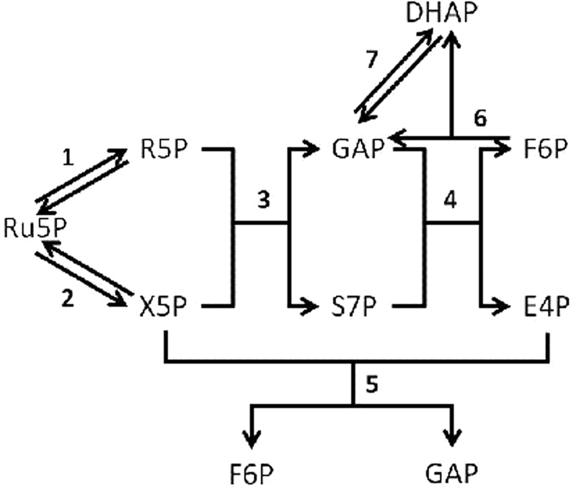
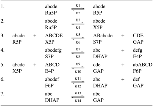
First, we can draw a schematic diagram of the pentose phosphate pathway (Fig. 1). From Figure 1, we can easily discover that the entire system contains eight metabolites and seven reactions. The eight metabolites are represented as A₁(Ru5P), A₂(R5P), A₃(X5P), A₄(S7P), A₅(GAP), A₆(F6p), A₇(E4P), and A₈(DHAP). The mechanisms of these seven reactions are listed in Table 1.

OPEN IN VIEWER

FIG. 1.

The process of the pentose phosphate pathway simulated in the model. Reaction 1 is Ru5P-R5P; reaction 2 is Ru5P-X5P; reaction 3 is R5P+X5P-S7P+GAP; reaction 4 is S7P-DHAP+E4P; reaction 5 is X5P+E4P-GAP+F6P; reaction 6 is F6P-DHAP+GAP; reaction 7 is DHAP-GAP. Details of the reaction are shown in reaction mechanism. DHAP, dihydroacetone phosphate; E4P, erythrose 4-phosphate; F6P, fructose 6-phosphate; GAP, glyceraldehyde 3-phospate; R5P, ribose 5-phosphate; Ru5P, ribulose 5-phosphate; S7P, sedoheptulose 7-phosphate; X5P, xylulose 5-phosphate.

OPEN IN VIEWER

Table 1.

The Mechanisms of The Seven Reactions

In Table 1, k_w is a constant indicating the chemical reaction rate, shown in Table 2 (Milstein and Bremermann, 1979).

In this pathway, by the analysis of the carbon atom's reaction mechanism in the entire process, we find that the first carbon atom (i.e., “a” in Table 1) in A₁ can transfer back to any position (i.e., a–e) in A₁. So the transfer process of each carbon atom is equivalent; this means Q¹=Q²=Q³=Q⁴=Q⁵. Then we can only calculate the value of Q¹. After simulating the transfer process of the first carbon atom, we find that it is hard to obtain the accurate probability of which product contains the first carbon atom if there are two or more products in the reaction. In fact, in the entire pathway, the rate of each reaction is different. So in this article, we distribute the probability by the ratio of products' factors in the reaction, that is, 1:1 in Table 1 obviously.

To test the effect of the MMFA approach, we evaluate the relative concentration through the reaction equilibrium constant (K) in Section 4.

4. Results

Using MATLAB, we input an initial concentration of A₁ and we got a group of probabilities when the system reached the steady state. Also we obtained the related concentration of each metabolism at the steady state. To test the approach, we selected the reaction equilibrium constant K to be the assessment indicator because each reaction in the pentose phosphate pathway is a reversible one.

The pentose phosphate pathway has been studied by many researchers (Kleijn et al., 2006; Luo et al., 2007; Zhao et al., 2008). Although it is simple and small, the most reactants and products in the pentose phosphate pathway are related with other metabolic systems. In this article, we selected the second, sixth, and seventh reactions to test the approach. Each K of these three reactions is listed in Table 3.

In MATLAB, we verified the initial concentration (defined as u) from 10 to 50 mmol/L and the distance value is 5 mmol/L, and the results are shown in Tables 4–6.

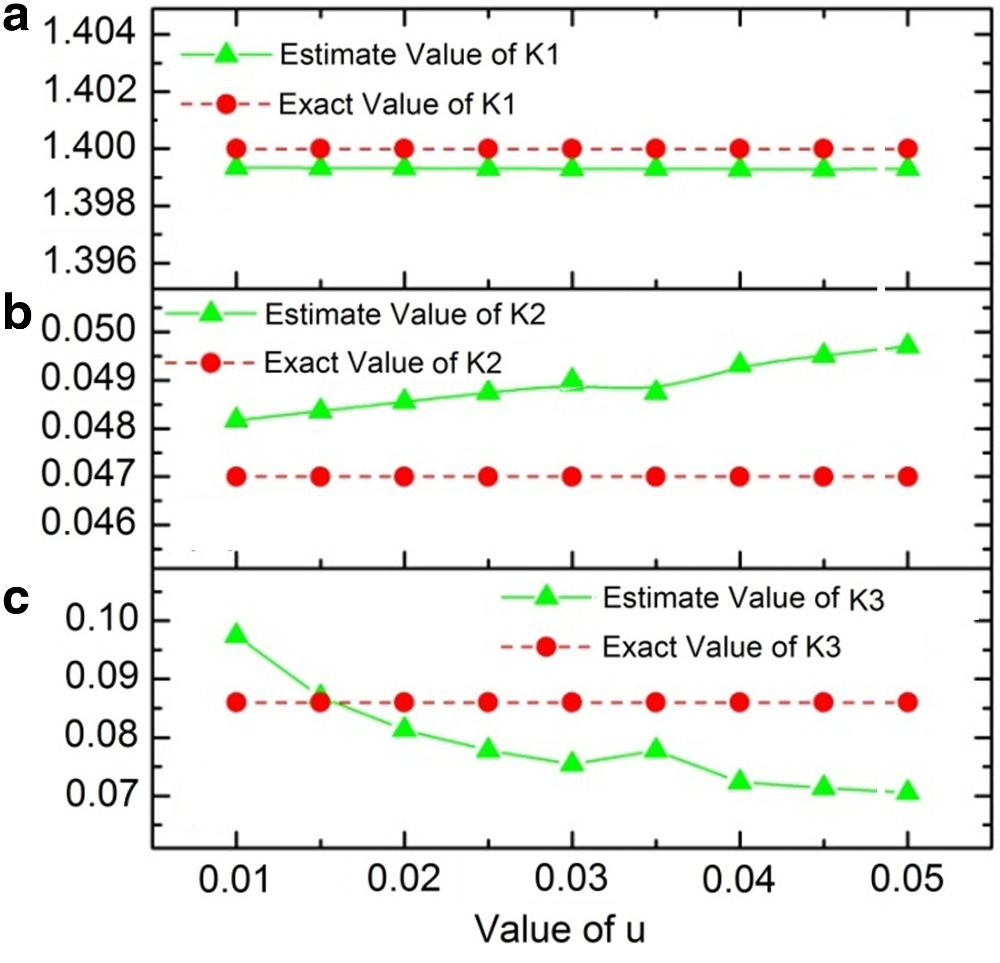
The results are also shown in Figure 2, where solid lines represent the estimation values of K₁, K₂, and K₃, while dotted lines are the exact values. From Figure 2a, the relative error of K₁ between the estimation value and the exact value is extremely small, so the estimation value is quite accurate. Also, the estimation value of K₂ is very close to its exact value, and its relative error is less than 6%, as seen in Table 5 and Figure 2b. The relative error of K₃ is a little more than K₁ and K₂; however, the estimation value is very close to its exact value. The relative error of K₃ is a little bit large because the corresponding metabolite F6P can also be produced by G6P in the entire metabolic system, but G6P is not included in the pentose phosphate pathway. In all, we can conclude that the results of this approach are quite reliable and accurate.

OPEN IN VIEWER

FIG. 2.

(a) The estimation value of K₁ when w changes from 10 to 50 mmol/L with the distance value of 5 mmol/L. (b) The estimation value of K₂ when u changes from 10 to 50 mmol/L with the distance value of 5 mmol/L. (c) The estimation value of K₃ when u changes from 10 to 50 mmol/L with the distance value of 5 mmol/L.

5. Conclusion

MFA is a powerful technique for determining intracellular metabolic fluxes in living cells. MFA has been found its widespread use in metabolic engineering, systems biology, biomedical research, and biotechnology.

In this article, a brand new approach, which combines MFA and continuous-time Markov chain, has been put forward to analyze metabolic flux in the metabolic system. On the basis of the study of the pentose phosphate pathway discussed in the Application section, this approach calculated the steady-state concentration by the distribution of each carbon atom. We obtained the reaction equilibrium constant for analysis and comparison, and found that this approach is feasible and the results are accurate. The approach proposed in this article is generic,mjm, which can be applied to any metabolic systems.