Enhancing Gibbs Sampling Method for Motif Finding in DNA with Initial Graph Representation of Sequences

Abstract

Finding short patterns with residue variation in a set of sequences is still an open problem in genetics, since motif-finding techniques on DNA and protein sequences are inconclusive on real data sets and their performance varies on different species. Hence, finding new algorithms and evolving established methods are vital to further understanding of genome properties and the mechanisms of protein development. In this work, we present an approach to finding functional motifs in DNA sequences in connection to Gibbs sampling method. Starting points in the search space are partly determined via graphical representation of input sequences opposed to completely random initial points with the standard Gibbs sampling. Our algorithm is evaluated on synthetic as well as on real data sets by using several statistics, such as sensitivity, positive predictive value, specificity, performance, and correlation coefficient. Additionally, a comparison between our algorithm and the basic standard Gibbs sampling algorithm is made to show improvement in accuracy, repeatability, and performance.

1. Introduction

According to steady scientific progression in technology and research in every field of natural sciences, the need for new solutions grows correspondingly, in biology as well as in other sciences. At the intersection of bioinformatics, genetics, computer science, and statistics one of the most prominent problems is the challenge of identifying and studying the translation mechanisms that regulate gene expressions in deoxyribonucleic acid (DNA). More specifically, the focus of corresponding studies are on specific regions of DNA strand called the promoter regions of transcription factors (TFs). Promoter regions present sequence signals upstream of each gene and thus function as target regions for an enzyme complex called RNA polymerase (RNAP) to bind and initiate the transcription of the gene into messenger RNA (mRNA). TFs can bind to the promoter regions and regulate gene expression by either inhibiting or enhancing the actions of RNAP (see Gupta and Liu, 2006).

TFs recognize sequence sites in DNA that give favorable binding energy, meaning a sequence-specific pattern, usually 8–20 base pairs long. Therefore this pattern, otherwise called a “motif,” is relatively well conserved in composition and is inscribed in the DNA as a variation of a sequence of four unique bases: adenine (A), thymine (T), cytosine (C), and guanine (G). Part of the DNA codes for assembly of amino acids, forming a polypeptide chain. The genetic code is read in a sequence of three bases called triplets on DNA, codons on mRNA, and anticodons on transfer RNA. There are 4³ = 64 triplets, and this is the smallest combination of four bases that could encode all 20 amino acids. The pioneers for the triplet code were Francis Crick and Sydney Brenner (Crick et al., 1961), who made an experiment that examined the effect of frame shift mutations on protein synthesis. Since then there was enough compelling evidence to infer that the genetic code is, in fact, a tree-based code (Smith, 2008).

To find the positions of motifs in DNA, various motif-finding algorithms were developed, and we can classify them into three categories: those that use promoter sequences from coregulated genes from a single genome, those that use orthologous promoter sequences of a single gene from multiple species (phylogenetic footprinting), and those that use both (Das and Dai, 2007). Further classification based on algorithm design places algorithms broadly into word-based algorithms (van Helden et al., 1998), probabilistic algorithms, and machine-learning techniques (Liu et al., 2006).

The probabilistic approach searches for the solution locally and represents the motif model by position weight matrix. One of the first implementations of this probabilistic scheme was with a greedy algorithm by Hertz et al. (1990), which evolved into a CONSENSUS algorithm (Hertz and Stormo, 1999). They introduced a method that evaluates an alignment through information content score based on large-deviation statistics. However, most probabilistic approaches use statistical techniques such as expectation–maximization (EM) methods and Gibbs sampling strategy. The former were used for identifying multiple motifs in biopolymer sequences with the MEME algorithm developed by Bailey and Elkan (1995).

Gibbs sampling, like the EM method, is an iterative procedure, where the results of every step depend solely on the result of the previous one. Unlike the EM method, the selection for the next step is not deterministic but rather based on random sampling, i.e., random numbers. Gibbs sampling for motif finding was first introduced by Lawrence et al. (1993), and since their publication various modifications to the algorithm were made, for instance, modeling for spaced dyads and motifs with palindromic patterns (Liu et al., 2001) using a probability distribution to estimate the number of copies of the motif per sequence and incorporation of higher order Markov-chain background model (Thijs et al., 2002), sequence weighting (Chen and Jiang, 2006), direct optimization of information content during sampling (Defrance and van Helden, 2009), among others.

In the subject of motif-finding algorithms, a term motif represents the conserved pattern, which is repetitive in the DNA strand. Thus a simple formulation of the problem is the following: in a given finite set of sequences, find an unknown motif that is over-represented. Statistically we can classify the motif-finding problem as a problem of missing data. The position of the motif element in a sequence, i.e., the elements of the alignment vector, can be treated as missing data (Gupta and Liu, 2006; Das and Dai, 2007; Liu et al., 2002).

In this article, we look for a solution differently by adding a preprocessing step before starting the iteration of the Gibbs sampler. Although the algorithm is based on Gibbs sampling strategy (Lawrence et al., 1993), we use graph representation of the sequences to help us project the local extremes in algorithm's search space. The sampling strategy is explained in more detail in the following section 2 and its application to multialignment problems in DNA sequences in section 2.1. In section 2.2, we describe the addition of graph representation and mention the points of difference from the original algorithm. In section 3, we detail the synthetic data sets and real data sets, which were gathered by Tompa et al. (2005), on which we tested our algorithm. The results are gathered in section 4, where we use statistics such as performance and correlation coefficient, sensitivity, and positive predictive value on nucleotide and site level to show the performance of our algorithm, which we named GraphGibbs. We conclude this article with section 5, where we summarize our findings and give some insight to future work.

2. The Method

The base of our algorithm is the original Gibbs sampling strategy for multiple alignment, as was introduced by Lawrence et al. (1993). We refer to it as the basic algorithm in the following text for simplicity, and we describe it briefly in the next subsection. The modifications we made are outlined in section 2.2.2.

Gibbs sampling is a particular case of Metropolis-Hastings algorithm, which, in turn, is an instance of a Markov chain Monte Carlo method (MCMC). The goal of the algorithm is to best approximate the distribution of unknown parameter, otherwise known as the target distribution. In our context, the unknown parameter is the alignment vector. The basic idea of how to approximate the target distribution is to construct a chain of states until convergence is reached. In construction, we invoke the Markov property, where the next state the chain visits, although determined by a probabilistic choice, depends only on the current state (first-order) or, in general, on the last m states (m-order). The starting point of the chain is usually arbitrary configuration of the unknown parameter (Resnik and Hardisty, 2010, Liu and Logvinenko, 2007).

2.1. Basic algorithm

Let K denote the number of residues in the alphabet of the sequences. The input of the basic algorithm is a set \documentclass{aastex}\usepackage{amsbsy}\usepackage{amsfonts}\usepackage{amssymb}\usepackage{bm}\usepackage{mathrsfs}\usepackage{pifont}\usepackage{stmaryrd}\usepackage{textcomp}\usepackage{portland, xspace}\usepackage{amsmath, amsxtra}\pagestyle{empty}\DeclareMathSizes{10}{9}{7}{6}\begin{document} $$\{S_1 , S_2 , \ldots , S_N \}$$ \end{document} of N sequences, either DNA (K = 4) or protein sequences (K = 20), and the width W of one motif, occurring once per sequence. The output is the final alignment of the most prominent motif in the given set.

The algorithm is initialized by choosing random starting positions within the various sequences, thus choosing a random starting motif alignment \documentclass{aastex}\usepackage{amsbsy}\usepackage{amsfonts}\usepackage{amssymb}\usepackage{bm}\usepackage{mathrsfs}\usepackage{pifont}\usepackage{stmaryrd}\usepackage{textcomp}\usepackage{portland, xspace}\usepackage{amsmath, amsxtra}\pagestyle{empty}\DeclareMathSizes{10}{9}{7}{6}\begin{document} $$a = (a_1 , \ldots , a_N)$$ \end{document} . Through many iterations, two steps of Gibbs sampler are executed: the predictive update step and the sampling step.

In the update step, one of the sequences, S_z, is chosen, either at random or in specified order. Then the elements of position weight matrix \documentclass{aastex}\usepackage{amsbsy}\usepackage{amsfonts}\usepackage{amssymb}\usepackage{bm}\usepackage{mathrsfs}\usepackage{pifont}\usepackage{stmaryrd}\usepackage{textcomp}\usepackage{portland, xspace}\usepackage{amsmath, amsxtra}\pagestyle{empty}\DeclareMathSizes{10}{9}{7}{6}\begin{document} $${\cal Q}$$ \end{document} and background description \documentclass{aastex}\usepackage{amsbsy}\usepackage{amsfonts}\usepackage{amssymb}\usepackage{bm}\usepackage{mathrsfs}\usepackage{pifont}\usepackage{stmaryrd}\usepackage{textcomp}\usepackage{portland, xspace}\usepackage{amsmath, amsxtra}\pagestyle{empty}\DeclareMathSizes{10}{9}{7}{6}\begin{document} $${\cal P} = [ p_j ] _{j = 1 , \ldots , K}$$ \end{document} are calculated from the current alignment a\{a_z} in all sequences excluding S_z. The elements of \documentclass{aastex}\usepackage{amsbsy}\usepackage{amsfonts}\usepackage{amssymb}\usepackage{bm}\usepackage{mathrsfs}\usepackage{pifont}\usepackage{stmaryrd}\usepackage{textcomp}\usepackage{portland, xspace}\usepackage{amsmath, amsxtra}\pagestyle{empty}\DeclareMathSizes{10}{9}{7}{6}\begin{document} $${\cal Q}$$ \end{document} matrix are calculated as \documentclass{aastex}\usepackage{amsbsy}\usepackage{amsfonts}\usepackage{amssymb}\usepackage{bm}\usepackage{mathrsfs}\usepackage{pifont}\usepackage{stmaryrd}\usepackage{textcomp}\usepackage{portland, xspace}\usepackage{amsmath, amsxtra}\pagestyle{empty}\DeclareMathSizes{10}{9}{7}{6}\begin{document} \begin{align*}q_ {i , j} = \frac {c_ {i , j} + b_j} {N - 1 + B} , \tag {1} \end{align*} \end{document}

where c_i,j is the count of residue j at position i in the motif, b_j is the pseudocount of residue j, and \documentclass{aastex}\usepackage{amsbsy}\usepackage{amsfonts}\usepackage{amssymb}\usepackage{bm}\usepackage{mathrsfs}\usepackage{pifont}\usepackage{stmaryrd}\usepackage{textcomp}\usepackage{portland, xspace}\usepackage{amsmath, amsxtra}\pagestyle{empty}\DeclareMathSizes{10}{9}{7}{6}\begin{document} $$B = \sum \nolimits_j b_j$$ \end{document} , for all \documentclass{aastex}\usepackage{amsbsy}\usepackage{amsfonts}\usepackage{amssymb}\usepackage{bm}\usepackage{mathrsfs}\usepackage{pifont}\usepackage{stmaryrd}\usepackage{textcomp}\usepackage{portland, xspace}\usepackage{amsmath, amsxtra}\pagestyle{empty}\DeclareMathSizes{10}{9}{7}{6}\begin{document} $$i = 1 , \ldots , W$$ \end{document} and \documentclass{aastex}\usepackage{amsbsy}\usepackage{amsfonts}\usepackage{amssymb}\usepackage{bm}\usepackage{mathrsfs}\usepackage{pifont}\usepackage{stmaryrd}\usepackage{textcomp}\usepackage{portland, xspace}\usepackage{amsmath, amsxtra}\pagestyle{empty}\DeclareMathSizes{10}{9}{7}{6}\begin{document} $$j = 1 , \ldots , K$$ \end{document} .

In the sampling step, every segment x of width W within sequence S_z is considered as a possible instance of the motif. According to position weight matrix \documentclass{aastex}\usepackage{amsbsy}\usepackage{amsfonts}\usepackage{amssymb}\usepackage{bm}\usepackage{mathrsfs}\usepackage{pifont}\usepackage{stmaryrd}\usepackage{textcomp}\usepackage{portland, xspace}\usepackage{amsmath, amsxtra}\pagestyle{empty}\DeclareMathSizes{10}{9}{7}{6}\begin{document} $${\cal Q}$$ \end{document} and background frequencies, motif probabilities \documentclass{aastex}\usepackage{amsbsy}\usepackage{amsfonts}\usepackage{amssymb}\usepackage{bm}\usepackage{mathrsfs}\usepackage{pifont}\usepackage{stmaryrd}\usepackage{textcomp}\usepackage{portland, xspace}\usepackage{amsmath, amsxtra}\pagestyle{empty}\DeclareMathSizes{10}{9}{7}{6}\begin{document} $$Q_x = P (x \mid {\cal Q})$$ \end{document} and \documentclass{aastex}\usepackage{amsbsy}\usepackage{amsfonts}\usepackage{amssymb}\usepackage{bm}\usepackage{mathrsfs}\usepackage{pifont}\usepackage{stmaryrd}\usepackage{textcomp}\usepackage{portland, xspace}\usepackage{amsmath, amsxtra}\pagestyle{empty}\DeclareMathSizes{10}{9}{7}{6}\begin{document} $$P_x = P (x \mid {\cal P})$$ \end{document} of segment x are calculated. Then the segment x is weighted with A_x = Q_x/P_x. From the weighted segments a random one is chosen with probability \documentclass{aastex}\usepackage{amsbsy}\usepackage{amsfonts}\usepackage{amssymb}\usepackage{bm}\usepackage{mathrsfs}\usepackage{pifont}\usepackage{stmaryrd}\usepackage{textcomp}\usepackage{portland, xspace}\usepackage{amsmath, amsxtra}\pagestyle{empty}\DeclareMathSizes{10}{9}{7}{6}\begin{document} $$A_x / \sum \nolimits_s A_s$$ \end{document} , where the sum is taken over all possible segments. The segment position prescribes the value to a_z.

The most probable alignment is chosen with the following score: \documentclass{aastex}\usepackage{amsbsy}\usepackage{amsfonts}\usepackage{amssymb}\usepackage{bm}\usepackage{mathrsfs}\usepackage{pifont}\usepackage{stmaryrd}\usepackage{textcomp}\usepackage{portland, xspace}\usepackage{amsmath, amsxtra}\pagestyle{empty}\DeclareMathSizes{10}{9}{7}{6}\begin{document} \begin{align*}F = \sum_ {i = 1} ^W \sum_ {j = 1} ^ {K} c_ {i , j} \log \frac {q_ {i , j}} {p_j} , \tag {2} \end{align*} \end{document}

where c_i_,j and q_i_,j are calculated from the complete alignment.

The authors Lawrence et al. (1993) also addressed the possibility in which a user parameter is a range of plausible motif widths, and let the algorithm decide the optimal one. They studied a statistic-named information per parameter \documentclass{aastex}\usepackage{amsbsy}\usepackage{amsfonts}\usepackage{amssymb}\usepackage{bm}\usepackage{mathrsfs}\usepackage{pifont}\usepackage{stmaryrd}\usepackage{textcomp}\usepackage{portland, xspace}\usepackage{amsmath, amsxtra}\pagestyle{empty}\DeclareMathSizes{10}{9}{7}{6}\begin{document} \begin{align*}I = \frac {F - \sum \nolimits_ {i = 1} ^N \left(\log L_i^ {\prime} + \sum \nolimits_ {j = 1} ^ {L_i^ {\prime}} Y_ {i , j} \log Y_ {i , j} \right)} {p} , \tag {3} \end{align*} \end{document}

where p is the number of free parameters, \documentclass{aastex}\usepackage{amsbsy}\usepackage{amsfonts}\usepackage{amssymb}\usepackage{bm}\usepackage{mathrsfs}\usepackage{pifont}\usepackage{stmaryrd}\usepackage{textcomp}\usepackage{portland, xspace}\usepackage{amsmath, amsxtra}\pagestyle{empty}\DeclareMathSizes{10}{9}{7}{6}\begin{document} $$L_i^{\prime}$$ \end{document} is the number of possible positions for the pattern within sequence i, and Y_i_,j is the normalized weight of position j.

2.2. Addition and adaptation

In this section, we describe our addition to the basic algorithm. It is a preprocessing step of the data gathered solely from DNA sequences that partly defines the initial point of iteration process. We apply a graph model constructed by given DNA sequences and analyze its adjacency matrix to determine motif candidates that are over-represented in the set of sequences. We also overview the modifications made to the basic algorithm.

2.2.1. Addition

Because Gibbs sampling conducts the search locally through parameter space, the starting point in the search space is not so trivial as it affects the speed of convergence of the sampler. The downside of searching only parts of the space, although through a probabilistic choice, is that the algorithm can get stuck in a local optimum or plateau. One solution would then be to make periodical shifts in the search space. Another improvement is the approximation of a possible starting point for the Gibbs sampler, instead of the random initialization starting values for unknown parameters. We consider both approaches in our algorithm.

Since the DNA code works with triplets as its base blocks, the intuition is to code the given set of sequences into triplets and use Gibbs sampling strategy on such coded sequences. The reading of triplets in the original sequences was done by moving one residue to the right. For instance, the sequence of AATCGTGGC is coded as AAT, ATC, TCG, CGT, GTG, TGG, GGC. Since we have a DNA alphabet of four residues, the number of triplets is 4³ = 64.

We take the input sequences and concatenate them into one supersequence R. Then we code the sequence R as described above and project it onto a directed multigraph G of order 64 (West, 2001). The vertices in G represent the triplets and are labeled by numbers 1 : 64, one number per triplet. The edge between two vertices in G reflect the adjacency between two consecutive triplets in R. Therefore, the number of edges between two vertices match the number of times the corresponding triplets are sequential in R. Each edge also has a direction, since we read the sequence R from left to right as the order of the triplets is important.

Once the sequence R is read and graph G constructed, we analyze the adjacency matrix of G. First we normalize it and then we look for the highest value in each row that can appear in more than one column. The reason is that the higher the number of directed multiple edges is between two vertices, the more frequent is the occurrence of sequence formed by these vertices inside the sequence R. We form (0, 1)-matrix, where the highest value of normalized adjacency matrix is represented by 1, and all other values are replaced by 0.

We sort the vertices in nonincreasing order per highest normalized values and select the front 10¹ vertices \documentclass{aastex}\usepackage{amsbsy}\usepackage{amsfonts}\usepackage{amssymb}\usepackage{bm}\usepackage{mathrsfs}\usepackage{pifont}\usepackage{stmaryrd}\usepackage{textcomp}\usepackage{portland, xspace}\usepackage{amsmath, amsxtra}\pagestyle{empty}\DeclareMathSizes{10}{9}{7}{6}\begin{document} $$v_1 , v_2 , \ldots , v_{10}$$ \end{document} . We are interested in the induced subgraph \documentclass{aastex}\usepackage{amsbsy}\usepackage{amsfonts}\usepackage{amssymb}\usepackage{bm}\usepackage{mathrsfs}\usepackage{pifont}\usepackage{stmaryrd}\usepackage{textcomp}\usepackage{portland, xspace}\usepackage{amsmath, amsxtra}\pagestyle{empty}\DeclareMathSizes{10}{9}{7}{6}\begin{document} $$H = G [ \{v_1 , v_2 , \ldots , v_{10} \} ]$$ \end{document} . Each vertex \documentclass{aastex}\usepackage{amsbsy}\usepackage{amsfonts}\usepackage{amssymb}\usepackage{bm}\usepackage{mathrsfs}\usepackage{pifont}\usepackage{stmaryrd}\usepackage{textcomp}\usepackage{portland, xspace}\usepackage{amsmath, amsxtra}\pagestyle{empty}\DeclareMathSizes{10}{9}{7}{6}\begin{document} $$v_s \in H$$ \end{document} is considered as the source vertex for a walk of length \documentclass{aastex}\usepackage{amsbsy}\usepackage{amsfonts}\usepackage{amssymb}\usepackage{bm}\usepackage{mathrsfs}\usepackage{pifont}\usepackage{stmaryrd}\usepackage{textcomp}\usepackage{portland, xspace}\usepackage{amsmath, amsxtra}\pagestyle{empty}\DeclareMathSizes{10}{9}{7}{6}\begin{document} $$\ell = \lceil{W / 2} \rceil - 3$$ \end{document} . Subgraph H can contain loops, thus the walks can be closed as well as open. Each walk reflects the succession of triplets in the sequence R and is a natural way to model over-represented patterns in R. A resembling idea using a graph model by Song et al. (2012) considers weighted cliques of a graph constructed from the input sequences. Each vertex in their graph represents a subsequence of length W, and each edge connects the vertices whose alignment score is higher than a certain threshold. However, we find a walk is more intuitive in modeling conservative patterns opposed to cliques, since it mirrors internal structure of input sequences.

We search for all walks of desired length with a modified breadth-first search algorithm (Cormen et al., 2001). While doing a systematic search of discoverable vertices from the source vertex v_s, the breadth-first algorithm also produces a breadth-first tree of size ℓ with root v_s that contains all reachable vertices. The modification makes the vertices discoverable more than once, opposed to at most once as in the basic breadth-first search algorithm. This way loops in the graph are also considered. Alongside the tree construction we also count the in-degree of each of the vertices. Then we consider the vertices of the highest in-degree together with their neighbor as a possible motif candidate.

From this motif candidate we build the motif in the following way: first we count the number of occurrences of the candidate in the input sequences. If their occurrence was at least N/2 times, then we would add the residues to each end of the candidate, until the number of motif occurrences is lower than N/2. In the case of undefined width W, the preferential feature is the motif width versus the number of occurrences. Therefore, the longer motif with less motif sites would be considered for further analysis, mainly because the shorter motifs are clustered inside the longer one and thus are not discarded. Once the motif is built we store the motifs positions in the alignment vector or matrix.

To help visualize the process, a representation of a (0, 1)-matrix is drawn in Fig. 1. The vertices are labeled with numbers 1 : 64, where each number represents a triplet. In this example, the motif width is W = 12. Then the length of the walk is ℓ = 3. One of the walks with source vertex 58 is drawn in blue color.

FIG. 1.

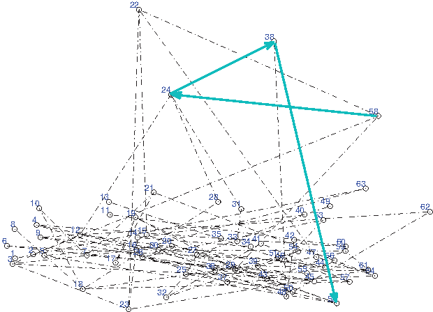
Graph representation of (0, 1)-matrix with one walk emphasized with blue color (v_s = 58).

This forms part one of our algorithm. When the vector a or matrix (in case of multiple sites per sequence) of the constructed motifs is not full, the second part of the algorithm, the Gibbs sampler, is executed. The first adaptation of the basic algorithm is the use of the site vector/matrix a to be the starting point of the Gibbs sampling algorithm. The algorithm pseudocode is given in Algorithm 1.

Algorithm 1

Pseudocode of the GraphGibbs algorithm.

Input: A set S of N DNA sequences

\documentclass{aastex}\usepackage{amsbsy}\usepackage{amsfonts}\usepackage{amssymb}\usepackage{bm}\usepackage{mathrsfs}\usepackage{pifont}\usepackage{stmaryrd}\usepackage{textcomp}\usepackage{portland, xspace}\usepackage{amsmath, amsxtra}\pagestyle{empty}\DeclareMathSizes{10}{9}{7}{6}\begin{document} $$S_1 , \ldots , S_N$$ \end{document}

Output: A motif of width W with the corresponding alignment a.

1: Code the sequences numerically into triplets.

2: Create the triplet's normalized adjacency matrix.

3: Search for all walks of 10 candidate vertices.

4: Take the vertices with the highest in-degree.

5: Build the motif from the starting candidate sextuple.

6: Remove the resulting motif from the sequences.

7: repeat

steps 2–6

8: until no more motifs

9: Take the found motif alignment

and fill it up with random values.

10: Choose a sequence S_z and exclude it from S, along with its site a_z from a.

11: Calculate

and

from S\{S_z}.

12: Weight every segment x in sequence S_z.

13: Take the segment x with the highest weight and assign new value to a_z = a_x.

14: repeat

steps 10–13

15: until convergence

return motif alignment a

2.2.2. Adaptation

The resulting alignment, determined by the parameter I, is displayed with triplets and with residues of the original DNA alphabet. In each case, the algorithm displays two motif consensuses. For one consensus, the triplet/residue with the highest probability (given by \documentclass{aastex}\usepackage{amsbsy}\usepackage{amsfonts}\usepackage{amssymb}\usepackage{bm}\usepackage{mathrsfs}\usepackage{pifont}\usepackage{stmaryrd}\usepackage{textcomp}\usepackage{portland, xspace}\usepackage{amsmath, amsxtra}\pagestyle{empty}\DeclareMathSizes{10}{9}{7}{6}\begin{document} $${\cal Q}$$ \end{document} matrix of the final alignment) is selected at each position in the motif. This way the full width motif is constructed and is the representative for the predicted motif. For the other consensus, the same threshold for all positions in the motif is considered. The value of the threshold was fixed through practical trials on different sets of data. The threshold for the coded motif is 0.65 and for the original alphabet is 0.85. At this value for each motif position the triplets/residues were indeed a part of the motif.

Another slight change is the way a new value of a_z in the temporary exempt sequence S_z is allocated in the sampling step. In our version, the value of a_z of the alignment vector is the start of the segment x that has the highest weight A_x, as opposed to random choosing. In the case of multiple motif sites per sequence, the sites of segments with the highest weights are chosen as the new sites in the alignment vector. The assumption is that after some steps of the Gibbs sampler the pattern should emerge by itself and would be reflected in the position weight matrix correspondingly. The weights of the segment mirror this evolution of the matrix, thus the most probable segments are chosen toward the final alignment.

3. Data

We tested our algorithm on several different cases of data. We considered the real data as well as synthetic data with known motifs. The real data sets used to test the algorithm are a part of the freely accessible benchmark data ensemble constructed by Tompa et al. (2005), which was analyzed with 13 different motif-finding algorithms according to their article. They build the data sets from real sequences gathered from TRANSFAC database. There were four species considered: yeast, fly, mouse, and human, resulting in 56 data sets. From yeast they constructed 8 data sets, 12 from mouse, 6 from fly, and 26 from human.

We also generated our own data sets, since they provide a well-controlled environment for evaluation of an algorithm. Because the motif sites are known, the evaluation statistics, sensitivity, and positive predictive value, among others, can be accurately computed, in contrast to real data sets, where some effective binding sites, even if predicted, could have escaped experimental detection and so are not considered as viable solutions. This makes predicted motifs harder to classify, as we cannot know whether the pattern is a part of the polynucleotide tract we can filter out, or it represents a possible functional motif. Even if predicted motifs are harder to classify, our algorithm will, under loose restraints, return all possible patterns (either consistent or nonconsistent) it finds in a set. Although, a reader should note that those patterns are statistically over-represented in the set and, if nothing more, could bear a closer examination of their viability. However, that distinction we leave to the user.

The synthetic data can be further divided into two groups. In each group the motifs are of known widths 9 and 12. In one group, these motifs are consistent, meaning the same pattern is repeated through all N sequences. In the other group, the pattern is inconsistent, allowing for different degrees of residue variation d(v). The highest degree of variation has value 3, applied in sets with motif width 12. In summary, we generated data sets per five different parameters, which are: the motif width \documentclass{aastex}\usepackage{amsbsy}\usepackage{amsfonts}\usepackage{amssymb}\usepackage{bm}\usepackage{mathrsfs}\usepackage{pifont}\usepackage{stmaryrd}\usepackage{textcomp}\usepackage{portland, xspace}\usepackage{amsmath, amsxtra}\pagestyle{empty}\DeclareMathSizes{10}{9}{7}{6}\begin{document} $$W \in \{9 , 12 \} $$ \end{document} , the sequence background length \documentclass{aastex}\usepackage{amsbsy}\usepackage{amsfonts}\usepackage{amssymb}\usepackage{bm}\usepackage{mathrsfs}\usepackage{pifont}\usepackage{stmaryrd}\usepackage{textcomp}\usepackage{portland, xspace}\usepackage{amsmath, amsxtra}\pagestyle{empty}\DeclareMathSizes{10}{9}{7}{6}\begin{document} $$L \in \{100 , 500 , 1000 , 2500 \} $$ \end{document} , the number of expected motif occurrences per sequence \documentclass{aastex}\usepackage{amsbsy}\usepackage{amsfonts}\usepackage{amssymb}\usepackage{bm}\usepackage{mathrsfs}\usepackage{pifont}\usepackage{stmaryrd}\usepackage{textcomp}\usepackage{portland, xspace}\usepackage{amsmath, amsxtra}\pagestyle{empty}\DeclareMathSizes{10}{9}{7}{6}\begin{document} $$E \in \{1 , 2 , 3 \} $$ \end{document} , the number of sequences in the set \documentclass{aastex}\usepackage{amsbsy}\usepackage{amsfonts}\usepackage{amssymb}\usepackage{bm}\usepackage{mathrsfs}\usepackage{pifont}\usepackage{stmaryrd}\usepackage{textcomp}\usepackage{portland, xspace}\usepackage{amsmath, amsxtra}\pagestyle{empty}\DeclareMathSizes{10}{9}{7}{6}\begin{document} $$N \in \{10 , 20 \} $$ \end{document} , and the degree of residue variation \documentclass{aastex}\usepackage{amsbsy}\usepackage{amsfonts}\usepackage{amssymb}\usepackage{bm}\usepackage{mathrsfs}\usepackage{pifont}\usepackage{stmaryrd}\usepackage{textcomp}\usepackage{portland, xspace}\usepackage{amsmath, amsxtra}\pagestyle{empty}\DeclareMathSizes{10}{9}{7}{6}\begin{document} $$d (v) \in \{0 , 1 , 2 , 3 \} $$ \end{document} .

4. Results

Each of the data sets was analyzed by the algorithm 10 times with all parameters fixed at values for the widest solution scope. In other words, the algorithm decides the number of motifs, their widths, and the number of occurrences per sequence by itself. These specifications were chosen to make the evaluation of algorithm performance equivalent across all data sets, since all data sets were run under the same conditions. Here we wanted to display how many of known motifs our algorithm can find in a set and how good these findings are. We condensed the results into several groups for clearer representation. In the results that follow we presented our algorithm's performance on these different collections to show how good the algorithm can detect known motifs and how distinctive that detection is.

4.1. Statistics

For each set, we have a list of known motifs with their positions in the sequences and a list of predictive motifs with their respective positions. We measured the algorithm performance using evaluation statistics on nucleotide and site levels. At the site level, we look for the overlap between the known and predicted motif positions. Accepted overlap is at least a quarter of known motif width. At this level we merely count the number of overlaps. At the nucleotide level, on the other hand, we determine how big the overlap actually is. Then we can define the common scores of true and false positives, along true and false negatives at nucleotide level as follows (Tompa et al., 2005):

• nTP—the number of nucleotide positions in both known and predicted sites,

• nFN—the number of nucleotide positions in known, but not in predicted, sites,

• nFP—the number of nucleotide positions not in known, but in predicted, sites and

• nTN—the number of nucleotide positions in neither known nor predicted sites.

Analogously, at site level we can define:

• sTP—the number of known sites overlapped by predicted sites,

• sFN—the number of known sites not overlapped by predicted sites, and

• sFP—the number of predicted sited not overlapped by known sites.

With these scores so defined, we can compute the following statistics:

i. Sensitivity: \documentclass{aastex}\usepackage{amsbsy}\usepackage{amsfonts}\usepackage{amssymb}\usepackage{bm}\usepackage{mathrsfs}\usepackage{pifont}\usepackage{stmaryrd}\usepackage{textcomp}\usepackage{portland, xspace}\usepackage{amsmath, amsxtra}\pagestyle{empty}\DeclareMathSizes{10}{9}{7}{6}\begin{document} \begin{align*}nSn = nTP / (nTP + nFN) \ {\rm and} \tag{4}\end{align*} \end{document} \documentclass{aastex}\usepackage{amsbsy}\usepackage{amsfonts}\usepackage{amssymb}\usepackage{bm}\usepackage{mathrsfs}\usepackage{pifont}\usepackage{stmaryrd}\usepackage{textcomp}\usepackage{portland, xspace}\usepackage{amsmath, amsxtra}\pagestyle{empty}\DeclareMathSizes{10}{9}{7}{6}\begin{document} \begin{align*}sSn = sTP / (sTP + sFN) , \tag{5}\end{align*} \end{document}

ii. Positive predictive value: \documentclass{aastex}\usepackage{amsbsy}\usepackage{amsfonts}\usepackage{amssymb}\usepackage{bm}\usepackage{mathrsfs}\usepackage{pifont}\usepackage{stmaryrd}\usepackage{textcomp}\usepackage{portland, xspace}\usepackage{amsmath, amsxtra}\pagestyle{empty}\DeclareMathSizes{10}{9}{7}{6}\begin{document} \begin{align*}nPPV = nTP / (nTP + nFP) \ {\rm and} \tag{6}\end{align*} \end{document} \documentclass{aastex}\usepackage{amsbsy}\usepackage{amsfonts}\usepackage{amssymb}\usepackage{bm}\usepackage{mathrsfs}\usepackage{pifont}\usepackage{stmaryrd}\usepackage{textcomp}\usepackage{portland, xspace}\usepackage{amsmath, amsxtra}\pagestyle{empty}\DeclareMathSizes{10}{9}{7}{6}\begin{document} \begin{align*}sPPV = sTP / (sTP + sFP) . \tag{7}\end{align*} \end{document}

At nucleotide level we can further compute:

iii. Specificity: \documentclass{aastex}\usepackage{amsbsy}\usepackage{amsfonts}\usepackage{amssymb}\usepackage{bm}\usepackage{mathrsfs}\usepackage{pifont}\usepackage{stmaryrd}\usepackage{textcomp}\usepackage{portland, xspace}\usepackage{amsmath, amsxtra}\pagestyle{empty}\DeclareMathSizes{10}{9}{7}{6}\begin{document} \begin{align*}nSP = nTN / (nTN + nFP) , \tag{8}\end{align*} \end{document}

iv. Performance coefficient: \documentclass{aastex}\usepackage{amsbsy}\usepackage{amsfonts}\usepackage{amssymb}\usepackage{bm}\usepackage{mathrsfs}\usepackage{pifont}\usepackage{stmaryrd}\usepackage{textcomp}\usepackage{portland, xspace}\usepackage{amsmath, amsxtra}\pagestyle{empty}\DeclareMathSizes{10}{9}{7}{6}\begin{document} \begin{align*}nPC = nTP / (nTP + nFN + nFP) , {\rm and} \tag{9}\end{align*} \end{document}

v. Correlation coefficient: \documentclass{aastex}\usepackage{amsbsy}\usepackage{amsfonts}\usepackage{amssymb}\usepackage{bm}\usepackage{mathrsfs}\usepackage{pifont}\usepackage{stmaryrd}\usepackage{textcomp}\usepackage{portland, xspace}\usepackage{amsmath, amsxtra}\pagestyle{empty}\DeclareMathSizes{10}{9}{7}{6}\begin{document} \begin{align*}nCC = \frac {nTP \cdot nTN - nFN \cdot nFP} {\sqrt {(nTP + nFN) (nTN + nFP) (nTP + nFP) (nTN + nFN)}} . \tag {10} \end{align*} \end{document}

At site level one can also look at the average performance, that is: \documentclass{aastex}\usepackage{amsbsy}\usepackage{amsfonts}\usepackage{amssymb}\usepackage{bm}\usepackage{mathrsfs}\usepackage{pifont}\usepackage{stmaryrd}\usepackage{textcomp}\usepackage{portland, xspace}\usepackage{amsmath, amsxtra}\pagestyle{empty}\DeclareMathSizes{10}{9}{7}{6}\begin{document} \begin{align*}sASP = (sSn + sPPV) / 2. \tag{11}\end{align*} \end{document}

4.2. Synthetic data

Results from the generated data sets were grouped according to motif width W, number of sequences in the data set N, and by motif consistency, where c represents a consistent motif and nc a nonconsistent motif. We labeled the group in a format of W_N_c/nc, for simplicity.

In each data set, we averaged the scores nTP, nFN, nFP, nTN, sTP, sFN, and sFP by number of repetition of a data set and calculated the statistics described in the previous subsection on both site and nucleotide levels. The results were then sorted in their respective group, where a weighted average for each of the seven scores was taken to calculate the statistics on both levels. In Fig. 2 below, the values of these statistics for each group are shown by bar chart on nucleotide level and by lines on the site level. Alongside eight distinctive groups we also show the values of statistics averaged across all analyzed data sets.

Fig. 2.

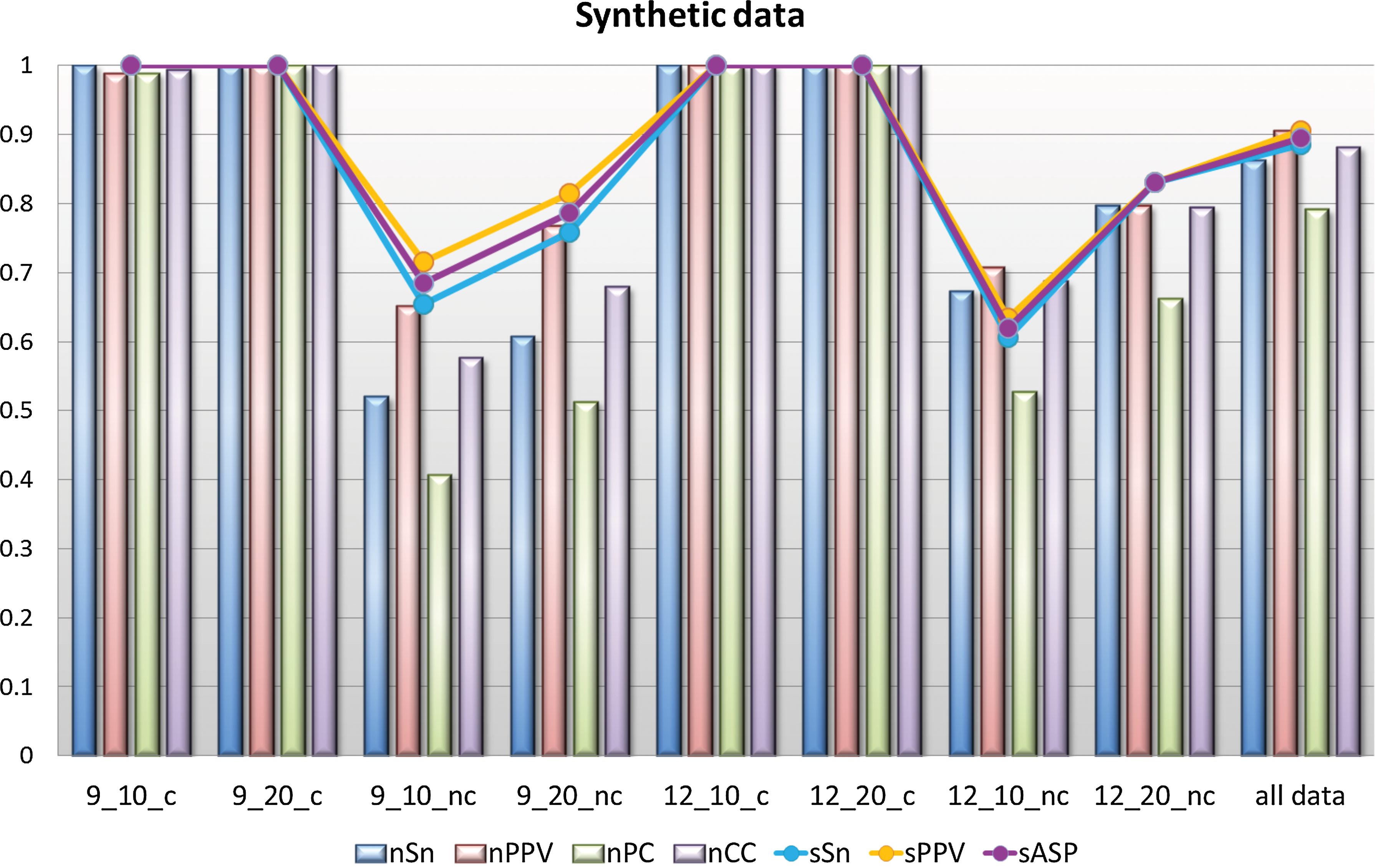
Combined representative statistics over eight groups of synthetic data.

The algorithm has shown good performance on sets with consistent motifs as expected, since the first part of the algorithm specifically searches for consistent, statistically over-represented motifs as candidates for the second part of the algorithm. Nearly all scores on both levels are at value 1, showing perfect correlation and high predictive power of the algorithm on sets containing consistent over-represented motif.

Naturally, more variability can be seen in groups with different degrees of variation. However, the nucleotide positive predictive values of all four groups, i.e., 9_10_nc, 9_20_nc, 12_10_nc, and 12_20_nc, are above 0.5 in two cases closer to 0.8. Therefore, there are not a lot of false positives among the predictions. Nucleotide sensitivity has slightly lower values comparing to nPPV but no lower than 0.5 in all four groups. Hence, the algorithm correctly predicted at least half of known motifs in all of the data sets.

Both of the correlation coefficients, nPC and nCC, are positive as well, giving a positive correlation between predicted and known sites. This is reflected on site level as well, since sSn and sPPV are both above the 0.6 threshold. The latter of the two has slightly higher values across all sets, meaning that the algorithm results in fewer false positives than false negatives.

4.3. Real data

To analyze the performance of the algorithm on real data, we chose the sets of type real of all four species from the data ensemble gathered by Tompa et al. (2005). The results from analyzed data sets were grouped by species, and the respective scores and statistics were calculated as with synthetic data. This way we gained four groups, and their statistics were computed from the weighted averages of the scores nTP, nFN, nFP, nTN, sTP, sFN, and sFP. Their values are drawn in Fig. 3 in the forms of a bar chart for nucleotide level and lines for site level.

Fig. 3.

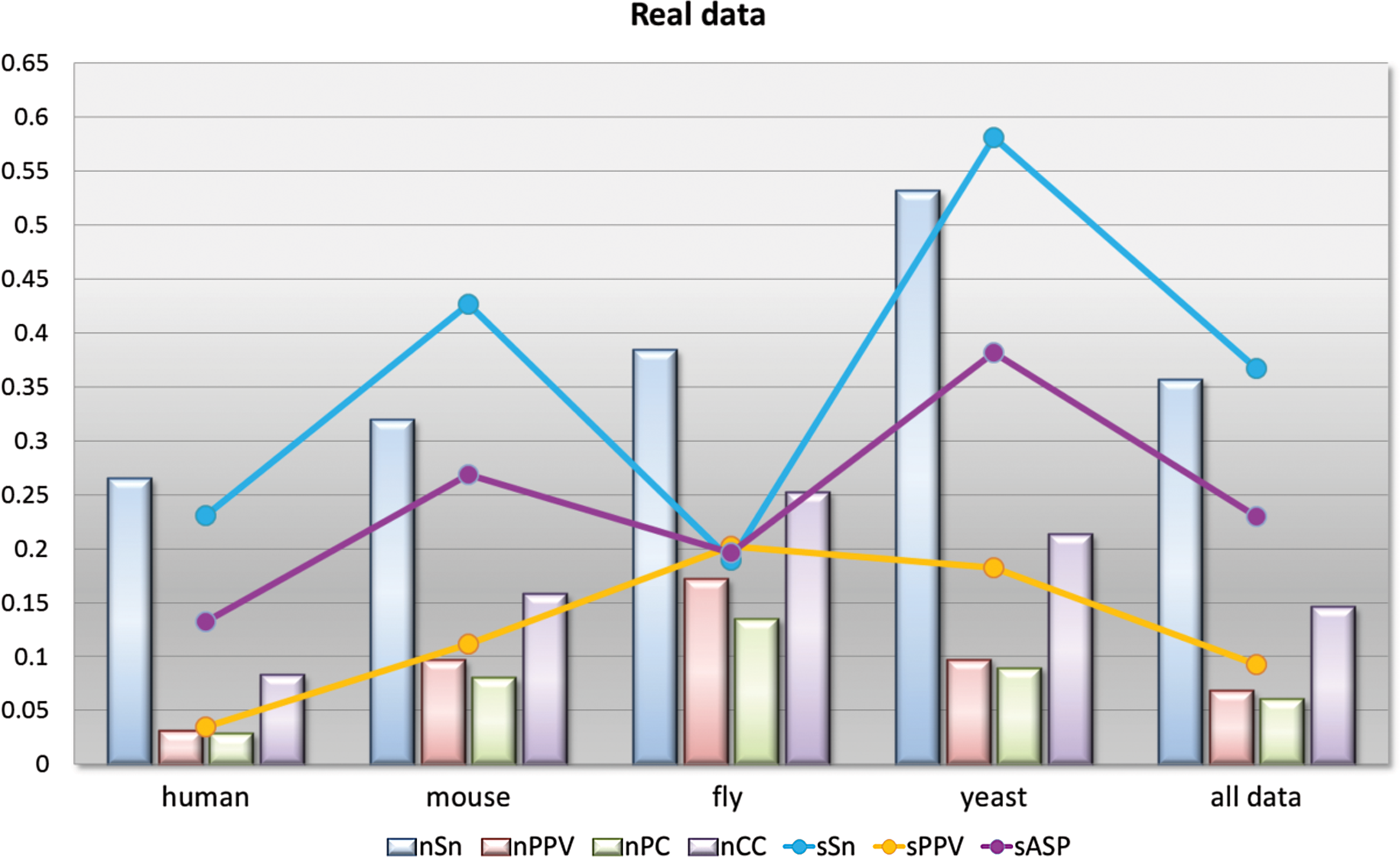
Combined representative statistics over real data sets grouped by species.

The sensitivity on both levels has higher values compared to positive predictive values. This implies that the algorithm makes more false negative predictions; that is, it does not identify all of the known nucleotide positions. These results, however, are a bit skewed because of the nature of the algorithm. With GraphGibbs algorithm the candidate motif tends to be of shorter width, since consistency in motifs is not occurring randomly in the set and drops radically when the width of the candidate motif increases.

Analogously the positive predictive values on both levels are a consequence of the algorithm setting, since the number of expected sites is uniform for all sequences. Thus, the algorithm predicts more sites compared to the actual number of occurrences per sequence of known motifs. Here one should also take into consideration that with real data the known motifs are experimentally determined and some motifs still need to be classified. Therefore, the number of false positives may be overstated, since the result can show an unknown functional motif. The interpretation we leave to the user.

Two statistics that reflect the algorithm's performance with more moderation are the correlation coefficient nCC and the average site performance sASP. The best results in the real data sets were for fly and yeast species. The former is more surprising, since the predictions on this set seems to be poorer compared to other sets (Tompa et al., 2005).

4.4. Additional statistical analysis

In Fig. 4 we show the specificity on nucleotide level, which is calculated from a weighted average of nucleotide scores of all data sets per group. It shows that true negatives are properly defined in most groups. There is an understandable dip with real data sets, however, it is not considerable. Here it is shown again that algorithm performance is best on the fly species. Notable are the higher values of human and mouse sets compared to yeast sets, although by a very small margin.

Fig. 4.

Specificity averaged across all data sets in the group.

To validate our algorithm, we compared the values of parameter I calculated from known and predicted alignment in selected generated sets. We took 4 and 6 sets of widths 9 and 12, respectively. In all of the sets the motifs are not consistent, L = 1000 and E = 1. The values of parameter I, averaged across 10 runs in each of 10 selected sets from predicted alignments of GraphGibbs and the basic algorithm, are shown in Table 1 alongside the value of I from known alignment. The average index of point of convergence is also added to the table to compare how fast the algorithm converges to the final alignment from partially determined initial alignment (GraphGibbs) versus completely random initial alignment (basic algorithm). The difference is small, however it does show that with GraphGibbs the convergence is faster.

Table 1.

Results and Performance Comparison Between GraphGibbs and the Basic Algorithm over 10 Runs on Each Set

Set	Known	GraphGibbs		Basic algorithm
W_d(v)_N	Parameter I	ParameterI	Point of convergence	ParameterI	Point of convergence
9_1_10	1.3783	1.3954	1.7	1.0582	3.9
9_2_10	1.1554	1.0657	2.4	1.082	3.8
9_1_20	2.5443	2.0826	1.5	1.8272	4.3
9_2_20	2.0226	1.6931	2.8	1.7924	5.4
	t-test	p = 0.14		p = 0.09
	%RSD	5.84		7.31
12_1_10	1.9475	2.0387	1.1	1.3213	4.8
12_2_10	1.6366	1.1472	1.9	0.9917	3.8
12_3_10	1.3766	1.0937	2	1.0287	5.1
12_1_20	3.9177	3.5923	1.8	2.1171	7.9
12_2_20	3.0802	1.3627	2	1.7629	5.2
12_3_20	2.5984	1.3167	7.2	1.6534	7.3
	t-test	p = 0.06		p < 0.05
	%RSD	13.71		35.6

RSD, relative standard deviation; boldface indicates significant difference.

To examine the accuracy (Zupan, 2009) of both algorithms, a paired two sample t-test for means of parameter I was performed on two groups differentiated by motif width. In the case of the GraphGibbs algorithm, the t-test shows no significant difference between the known and predicted alignment. The corresponding p-value (two tail) shows no statistically significant difference for neither first group, W = 9 (p = 0.14), nor the second group, W = 12 (p = 0.06). Meanwhile, for basic algorithm the t-test showed no significant difference where W = 9 (p = 0.09), but there is a significant difference (p < 0.05) in the second group. To emphasize significant differences, a boldface font was used in Table 1.

Since each set was run 10 times with both algorithms, we calculated the relative standard deviation (%RSD) of parameter I on both groups to measure repeatability (Zupan, 2009). The values for both groups are lower in the case of GraphGibbs opposed to values gained from the basic algorithm. The dispersion in the second group is higher due to the lower accuracy and higher degree of residue variation. In this group the difference between values of %RSD is more noticeable as well, because of the random sampling of the basic algorithm.

The time component of the two algorithms was compared in regards to site sensitivity. Both properties were averaged across 10 runs. For each algorithm the results were further divided by N, since larger sets are expected to have longer execution time. Figure 5 shows that basic algorithms have shorter execution time compared to GraphGibbs, however, the site sensitivity of the basic algorithm is very low. In contrast, GraphGibbs has higher average site sensitivity, although it takes longer to execute. This is also expected, since GraphGibbs builds upon the basic algorithm and has a wider search criteria.

Fig. 5.

Site sensitivity in relation to execution time of GraphGibbs and the basic algorithm on 10 sets. The sets are further grouped by N.

5. Conclusions

In this article, we explore another way of finding relevant motifs in DNA sequences. We build upon a Gibbs sampling method to help determine the regions of search space, which are more likely to contain a global extreme, consequently increasing accuracy of the predicted motifs.

The statistics have shown that GraphGibbs algorithm does enhance the basic algorithm of Gibbs sampling in terms of site sensitivity and faster convergence of the sampling method. It's performance on generated data sets is good even on sets with nonconsistent motifs at various degrees of residue variation. GraphGibbs also detected motifs in real data sets, although the sPPV was lower on most data sets compared to sSn. As discussed above, this is in part a consequence of algorithm setting, since the expected number of motif occurrences is uniform for all sequences. Hence the alignment N × E matrix is full and results in more false positives. In addition, the motifs in real sets are determined experimentally and some functional motifs of interest may have escaped detection and classification. Thus, the resulting values of sPPV may be perceived lower than in cases of fully analyzed real sequences.

To help improve the accuracy of our algorithm, we are focusing on reducing the number of false positives by considering nonuniform distribution of expected numbers of sites through the set. This means that we have to look at the number of motif occurrences individually per sequence. We are exploring a probability distribution to help estimate the number of copies of a motif per sequence as was introduced by Thijs et al. (2002). Another modification in progress is a motif-ranking procedure to rank all motifs found by the algorithm. Additionally, we want to mitigate the limitation on motif width of predicted motifs, a consequence of part one of the algorithm, where consistent motifs are being detected and those are usually short. This way we would lower the number of false negatives on nucleotide level.

Since the GraphGibbs algorithm is essentially trying to find patterns composed with a specific alphabet, the algorithm could be applied to pattern recognition problems with structured patterns outside of biology and genetics, with slight adaptation to the new alphabet and inherent properties of the data set.

Footnotes

Acknowledgments

The author thanks Damjana Kokol Bukovšek, Matjaž Omladič, Alenka Stepančič, and Gregor Šega for their guidance and help with the development and analysis of the algorithm. The author also thanks Arctur d.o.o. for technical support and access to the supercomputer Arctur-1 for algorithm execution. This work was supported in part by the European Union, European Social Fund. The real data set gathered by Tompa et al. () can be accessed online.

Author Disclosure Statement

No competing financial interests exist.

1

The choice of number of vertices is arbitrary, however, we found that usually around ten vertices stand out with higher degree compared to the rest.

References

Bailey

, and Elkan

1995. Unsupervised learning of multiple motifs in biopolymers using expectation maximization. Machine Learning, 21, 50–83.

Chen

, and Jiang

2006. An improved Gibbs sampling method for motif discovery via sequences weighting, 239–247. In Markstein

, and Xu

, eds. Computational Systems Bioinformatics. Imperial College Press, Stanford, California.

Cormen

, et al. 2001. Introduction to Algorithms. 2nd ed. The MIT Press, Cambridge, England.

Crick

, Barnett

, Brenner

, et al. 1961. General nature of the genetic code for proteins. Nature, 4809, 1227–1232.

Das

, and Dai

2007. A survey of DNA motif finding algorithms. BMC Bioinformatics, 8. Suppl. 7.

Defrance

, and van Helden

2009. info-gibbs: a motif discovery algortihm that directly optimized information content during sampling. Bioinformatics, 25, 2715–2722.

Gupta

, and Liu

2006. Bayesian inference for gene expression and proteomics. Cambridge University Press, Cambridge.

Hertz

, Hartzell

, and Stormo

1990. Identification of consensus patterns in unaligned DNA sequences known to be functionally related. Comput. Appl. Biosci., 6, 81–92.

Hertz

, and Stormo

1999. Identifying DNA and protein patterns with statistically significant alignments of multiple sequences. Bioinformatics, 15, 563–577.

10.

Lawrence

, Altschul

, Bogunski

, et al. 1993. Detecting subtle sequence signals: a gibbs sampling strategy for multiple alignment. Science, 8, 208–214.

11.

Liu

, Xiong

, DasGupta

, et al. 2006. Motif discoveries in unaligned molecular sequences using self-organizing neural networks. IEEE Trans. Neural Networks, 17, 919–928.

12.

Liu

, Gupta

, Liu

, et al. 2002. Statistical models for biological sequence motif discovery, 1–18. In Gatsonis

, Kass

, Carriquiry

, et al., eds. Case Studies in Bayesian Statistics. Carnegie Mellon University, Pittsburg, Pennsylvania.

13.

Liu

, and Logvinenko

2007. Appendix A: Markov chain Monte Carlo methods, 91–92. In Balding

, Bishop

, and Cannings

, eds. Handbook of Statistical Genetics, 3rd ed. John Wiley & Sons Ltd, Hoboken, New Jersey.

14.

Liu

, Brutlag

, and Liu

2001. Bioprospector: Discovering conserved DNA motifs in upstream regulatory regions of co-expressed genes. Pac. Symp. Biocomput. 6, 127–138.

15.

Resnik

, and Hardisty

2010. Gibbs sampling for the uninitiated. Tech. Rep. LAMP-TR-153, Department of Linguistics, Institute for Advanced Computer Studies, University of Maryland, College Park, Maryland.

16.

Smith

2008. Nucleic acids to amino acids: DNA specifies protein. Nature Education, 1, 126.

17.

Song

, James

, and Chi

2012. A new approach for identifying transcription factor binding sites. International Journal of Science & Informatics, 2, 15–22.

18.

Thijs

, Marchal

, Lescot

, et al. 2002. A Gibbs sampling method to detect overrepresented motifs in the upstream regions of coexpressed genes. J. Comp. Biol., 9, 447–464.

19.

Tompa

, Li

, Bailey

, et al. 2005. Assessing computational tools for the discovery of transcriptions factor binding sites. Nature Biotechnology, 23, 137–144.

20.

van Helden

, André

, and Collado-Vides

1998. Extracting regulatory sites from the upstream region of yeast genes by computational analysis of oligonucleotide frequencies. J. Mol. Biol., 281, 827–842.

21.

West

2001. Introduction to Graph Theory, 2nd ed. Pearson Education, Inc., Delhi, India.

22.

Zupan

2009. Kemometrija in obdelava eksperimentalnih podatkov. Inštitut Nove Revije, Zavod za humanistiko in Kemijski inštitut Ljubljana, Ljubljana.