Characterizing the Empirical Distribution of Prokaryotic Genome n -mers in the Presence of Nullomers

Abstract

Characterizing the empirical distribution of the frequency of n-mers is a vital step in understanding the entire genome. This will allow for researchers to examine how complex the genome really is, and move beyond simple, traditional modeling frameworks that are often biased in the presence of abundant and/or extremely rare words. We hypothesize that models based on the negative binomial distribution and its zero-inflated counterpart will characterize the n-mer distributions of genomes better than the Poisson. Our study examined the empirical distribution of the frequency of n-mers (6 ≤ n ≤ 11) in 2,199 genomes. We considered four distributions: Poisson, negative binomial, zero-inflated Poisson, and zero-inflated negative binomial (ZINB). The number of genomes that have nullomers in 6-, 7-, and 8-mers was 150, 602 and 2,012, respectively, whereas all of the genomes for the 9-, 10-, and 11-mers had nullomers. In each n-mer considered, the negative binomial model performed the best for at least 93% of the 2,199 genomes; however, a small percentage (i.e., <7%) of the genomes did prefer the ZINB. The negative binomial and zero-inflation distributions extend the traditional Poisson setting and are more flexible in handling overdispersion that can be caused by an increase in nullomers. In an effort to characterize the distribution of the frequency of n-mers, researchers should also consider other discrete distributions that are more flexible and adjust for possible overdispersion.

1. Introduction

DNA n-mers, which are DNA “words” of length n, and their corresponding distributions in the entire genome sequence have been examined for some time now, and there has been a recent focus on finding significantly under- or overrepresented words. The empirical frequencies of these n-mers provide a perspective of genome complexity and their statistical properties, which is important for evolutional biology (Fofanov et al., 2004), and several methods have been proposed in characterizing the distribution of these words. Reinert et al. (2000) examined various distributions and showed that there are two distinct large sample regimes: a normal distribution for abundant n-mers and a Poisson or compound Poisson distribution for extremely rare n-mers. Robin and Schbath (2001) also outline the use of exact distributions as well as Gaussian approximations; Robin (2002) then expounded on using compound Poisson modeling for word occurrences in DNA sequences. This study used modeling to take into account the frequency of the words and their overlapping structure, where the compound Poisson model was compared to Markov chain modeling.

Nullomers are short DNA sequences that are absent from genomes of humans and other species (Acquisti et al., 2007), and the discovery of these nullomers is somewhat surprising when one considers that the genomes of higher organisms are extremely large (Kidwell, 2002). Hampikian and Andersen (2006) carried out a systematic study of these nullomers, and their work was motivated by the lack of research in examining these universally absent sequences in the hope of discovering insights into the most conserved mechanisms of molecular biology. This work focused on reporting the list of missing n-mers in 12 species, including humans. Nullomers play an important role when classifying prokaryotic sequences, and the naïve Bayes classifier can use a heuristic “linguistic smoothing” to make a better estimate of a nullomer (Chen and Goodman, 1996; Rosen et al., 2008). However, as the amount of genomes available grows, a more accurate estimate can be obtained from a better model of the genome n-mer distribution. Although some work has been done in characterizing the empirical distribution of these nullomers, the noted literature generally focuses on either Gaussian approximations or Poisson processes, and we aim to improve upon this body of work.

Several discrete distributions can be considered when describing the frequency of any DNA word in a given genome, but when overdispersion is present, traditional Poisson processes may not be appropriate. Overdispersion could be present for a variety of reasons, such as excessive zeros and outliers; therefore, distributions like the negative binomial allow for the extra variability present in the count data. To accommodate zero inflation in count data, zero-inflated models also have been developed (Lambert, 1992).

The purpose of this study is to characterize the distribution of the unique n-mer (6 ≤ n ≤ 11) frequency profiles of 2,199 microbial genomes, publicly available as of December 2012. The Materials and Methods section outlines the characteristics of each discrete distribution, as well as the statistical analysis used in examining the 2,199 genomes. In the Results and Discussion section of the article, we describe the empirical distribution of the n-mers and then compare the various discrete distributions (i.e., Poisson, negative binomial, zero-inflated Poisson [ZIP], and zero-inflated negative binomial [ZINB]) presented via Akaike information criterion (AIC) in order to determine the best probabilistic model fit. We also discuss the advantages and disadvantages of each distribution. Finally, the Conclusion section summarizes our main findings and details their importance and relevance.

2. Materials and Methods

We obtained DNA sequences for 2,199 prokaryotic genomes from GenBank (Benson et al., 2012) as of December 2012. The 2,199 genomes were marked as “completed” in the microbial genomes database. For each genomic sequence, the total number of possible n-mers is 4ⁿ. Because we are interested only in fitting low-order Markov models, such as zero-order Markov models, only the frequencies of each nucleotide for a given genome are needed (Chor et al., 2009). We systematically examined four discrete distributions to characterize the behavior of each n-mer (6 ≤ n ≤ 11) frequency. The distributions are outlined below, and the description of our statistical analyses follows.

2.1. Poisson

The Poisson distribution is commonly used to characterize count data. For example, if one is interested in modeling a setting where we are waiting for an occurrence (i.e., waiting for a bus), the number of occurrences in a given time interval can be modeled by this type of distribution. A random variable X, taking values in the nonnegative integers, has a Poisson distribution if \documentclass{aastex}\usepackage{amsbsy}\usepackage{amsfonts}\usepackage{amssymb}\usepackage{bm}\usepackage{mathrsfs}\usepackage{pifont}\usepackage{stmaryrd}\usepackage{textcomp}\usepackage{portland, xspace}\usepackage{amsmath, amsxtra}\pagestyle{empty}\DeclareMathSizes{10}{9}{7}{6}\begin{document} \begin{align*}P ( X = x \mid \lambda ) = \frac { e^ { - \lambda } \lambda^x } { x! } , \quad x = 0 , 1 , \ldots\end{align*} \end{document}

where λ is termed the intensity parameter. A distinct characteristic of this distribution is the fact that the mean and the variance are both equal to λ; therefore, E(X) = V(X) = λ (Casella and Berger, 1990). Unfortunately, when the variance significantly exceeds the mean, overdispersion is present, and this distribution will no longer be appropriate to use. Lastly, one can obtain the moment generating function for the Poisson distribution via a Taylor series, such that \documentclass{aastex}\usepackage{amsbsy}\usepackage{amsfonts}\usepackage{amssymb}\usepackage{bm}\usepackage{mathrsfs}\usepackage{pifont}\usepackage{stmaryrd}\usepackage{textcomp}\usepackage{portland, xspace}\usepackage{amsmath, amsxtra}\pagestyle{empty}\DeclareMathSizes{10}{9}{7}{6}\begin{document} $$M_x ( t ) = e^{ \lambda ( e^t - 1 ) }$$ \end{document} .

2.2. Negative binomial

The negative binomial distribution is also commonly used to characterize count data, except that this setting focuses on counting the number of Bernoulli trials required to get a fixed number of successes (Casella and Berger, 1990). Assuming a sequence of independent Bernoulli (p) trials, where p is the rate of success, the random variable X denotes the number of trials before the rth success occurs. X has a negative binomial distribution, such that \documentclass{aastex}\usepackage{amsbsy}\usepackage{amsfonts}\usepackage{amssymb}\usepackage{bm}\usepackage{mathrsfs}\usepackage{pifont}\usepackage{stmaryrd}\usepackage{textcomp}\usepackage{portland, xspace}\usepackage{amsmath, amsxtra}\pagestyle{empty}\DeclareMathSizes{10}{9}{7}{6}\begin{document} \begin{align*}P ( X = x \mid r , p ) = {r + x - 1 \choose x}p^r ( 1 - p ) ^x , \quad x = 0 , 1 , \ldots\end{align*} \end{document}

The name of this distribution comes from the relationship and defining equation for binomial coefficients with negative integers (Feller, 2008), where \documentclass{aastex}\usepackage{amsbsy}\usepackage{amsfonts}\usepackage{amssymb}\usepackage{bm}\usepackage{mathrsfs}\usepackage{pifont}\usepackage{stmaryrd}\usepackage{textcomp}\usepackage{portland, xspace}\usepackage{amsmath, amsxtra}\pagestyle{empty}\DeclareMathSizes{10}{9}{7}{6}\begin{document} \begin{align*} { r + x - 1 \choose x } = ( - 1 ) ^x \frac { ( - r ) ( - r - 1 ) ( - r - 2 ) \ldots ( - r - x + 1 ) } { ( x ) ( x - 1 ) ( x - 2 ) \ldots ( 2 ) ( 1 ) } .\end{align*} \end{document}

Substituting this relationship into the negative binomial distribution results in \documentclass{aastex}\usepackage{amsbsy}\usepackage{amsfonts}\usepackage{amssymb}\usepackage{bm}\usepackage{mathrsfs}\usepackage{pifont}\usepackage{stmaryrd}\usepackage{textcomp}\usepackage{portland, xspace}\usepackage{amsmath, amsxtra}\pagestyle{empty}\DeclareMathSizes{10}{9}{7}{6}\begin{document} \begin{align*}P ( X = x \mid r , p ) = ( - 1 ) ^x{ - r \choose x}p^r ( 1 - p ) ^x.\end{align*} \end{document}

The mean of this distribution is \documentclass{aastex}\usepackage{amsbsy}\usepackage{amsfonts}\usepackage{amssymb}\usepackage{bm}\usepackage{mathrsfs}\usepackage{pifont}\usepackage{stmaryrd}\usepackage{textcomp}\usepackage{portland, xspace}\usepackage{amsmath, amsxtra}\pagestyle{empty}\DeclareMathSizes{10}{9}{7}{6}\begin{document} $$E ( X ) = \frac { r ( 1 - p ) } { p } $$ \end{document} , and the variance is \documentclass{aastex}\usepackage{amsbsy}\usepackage{amsfonts}\usepackage{amssymb}\usepackage{bm}\usepackage{mathrsfs}\usepackage{pifont}\usepackage{stmaryrd}\usepackage{textcomp}\usepackage{portland, xspace}\usepackage{amsmath, amsxtra}\pagestyle{empty}\DeclareMathSizes{10}{9}{7}{6}\begin{document} $$V ( X ) = \frac { r ( 1 - p ) } { p^2 } $$ \end{document} . The negative binomial family of distributions includes the Poisson distribution as a limiting case, such that, if r → ∞ and p → 1, where r(1−p) → λ, then E(X) = r(1−p) → λ and V(X) = r(1−p) → λ. The advantage of using this distribution as opposed to the Poisson distribution is that the mean and variance are not required to be equivalent; in turn, this distribution allows one to measure the amount of possible overdispersion present.

2.3. Zero-inflated Poisson

Lambert (1992) first introduced the ZIP, although Mullahy (1986) initially explored the specification and testing of some modified count data models like the Poisson, while others have discussed this issue in detail (Cohen, 1963; Johnson and Kotz, 1969). Excessive zeros can occur in various settings, such as in manufacturing equipment that is properly aligned and defects are nearly impossible. This distribution provides an environment for modeling excessive zero counts in addition to positive counts. More specifically, this mixture model allows each count to have two possible generating processes, often called states, where a Bernoulli trial determines which processes the observed count follows. A ZIP assumes two states: (1) a perfect zero state and (2) an imperfect state. The perfect state allows only for the count to equal 0 with a certain probability, whereas the imperfect state allows each count to follow the Poisson distribution with another probability, such that X∼0 with probability π for the perfect state and X∼Poisson(λ) with probability (1−π). Therefore, the ZIP distribution is as follows: \documentclass{aastex}\usepackage{amsbsy}\usepackage{amsfonts}\usepackage{amssymb}\usepackage{bm}\usepackage{mathrsfs}\usepackage{pifont}\usepackage{stmaryrd}\usepackage{textcomp}\usepackage{portland, xspace}\usepackage{amsmath, amsxtra}\pagestyle{empty}\DeclareMathSizes{10}{9}{7}{6}\begin{document} \begin{align*}X = \begin{cases} 0 , { \rm with \ probability } \ \pi + ( 1 - \pi ) e^ { - \lambda } \\ x , { \rm with \ probability } \ ( 1 - \pi ) \frac { e^ { - \lambda } \lambda^x } { x! } , \ x = 1 , 2 , \ldots \end{cases} \end{align*} \end{document}

The advantage of this distribution and its corresponding regression is that it inflates the number of zeros by mixing a point mass at 0 with a Poisson distribution, and it is an extremely practical way to model count data with both excessive zeros and large counts that may appear as outliers.

2.4. Zero-inflated negative binomial

The ZINB distribution has a mixture form, similar to the ZIP distribution. This mixture distribution allows for a more flexible environment to handle overdispersion, where the nonzero counts can assume a zero-truncated negative binomial distribution. The ZINB distribution is as follows: \documentclass{aastex}\usepackage{amsbsy}\usepackage{amsfonts}\usepackage{amssymb}\usepackage{bm}\usepackage{mathrsfs}\usepackage{pifont}\usepackage{stmaryrd}\usepackage{textcomp}\usepackage{portland, xspace}\usepackage{amsmath, amsxtra}\pagestyle{empty}\DeclareMathSizes{10}{9}{7}{6}\begin{document} \begin{align*}X = \begin{cases} 0 , { \rm with \ probability} \ \pi + ( 1 - \pi ) p^r \\ x , { \rm with \ probability} \ ( 1 - \pi ) {r + x - 1 \choose x} \ p^r ( 1 - p ) ^x , \ x = 1 , 2 , \ldots\end{cases}\end{align*} \end{document}

where \documentclass{aastex}\usepackage{amsbsy}\usepackage{amsfonts}\usepackage{amssymb}\usepackage{bm}\usepackage{mathrsfs}\usepackage{pifont}\usepackage{stmaryrd}\usepackage{textcomp}\usepackage{portland, xspace}\usepackage{amsmath, amsxtra}\pagestyle{empty}\DeclareMathSizes{10}{9}{7}{6}\begin{document} $$p = \frac { r } { r + \mu } $$ \end{document} and μ is the mean of the underlying negative binomial distribution. The mean of the ZINB is E(X) = (1−π)μ, where the variance is \documentclass{aastex}\usepackage{amsbsy}\usepackage{amsfonts}\usepackage{amssymb}\usepackage{bm}\usepackage{mathrsfs}\usepackage{pifont}\usepackage{stmaryrd}\usepackage{textcomp}\usepackage{portland, xspace}\usepackage{amsmath, amsxtra}\pagestyle{empty}\DeclareMathSizes{10}{9}{7}{6}\begin{document} $$V ( X ) = ( 1 - \pi ) ( 1 + \mu / r + \pi \mu ) \mu$$ \end{document} . As r → ∞ , the ZINB simplifies to ZIP distribution (Yau et al., 2003).

2.5. Statistical approach

In this study, we are interested in moving beyond the traditional Poisson setting that is often used to characterize the distribution of these DNA words, especially in the presence of overdispersion that may be caused by a significant number of absent words. Our analyses were carried out in two steps, where the first step involved utilizing graphical techniques. Similar to Chor et al. (2009), we looked at the histograms of various genomes in an effort to visually assess the empirical distributions. It allowed us to determine a few things: Is there a spike at zero, and is there a significant amount of skewness in the right tail? We were also interested in the percentage of absent words present, since we hypothesized that the number of nullomers would increase as the size of each n-mer increased. After these initial analyses, our second step involved fitting the data using regression-based models with only a fixed intercept, assuming the various distributions outlined above.

To select a good model in terms of estimating quantities of interest, we chose to use the AIC (Akaike, 1974). In comparing simple versus more complex models, a simple model may be more parsimonious and result in better estimates of the certain characteristics of the true model; however, it may actually be farther from the true model than a more complex model. The AIC statistic judges a model by how close its fitted values tend to be to the true values with respect to a certain expected value. It is defined as \documentclass{aastex}\usepackage{amsbsy}\usepackage{amsfonts}\usepackage{amssymb}\usepackage{bm}\usepackage{mathrsfs}\usepackage{pifont}\usepackage{stmaryrd}\usepackage{textcomp}\usepackage{portland, xspace}\usepackage{amsmath, amsxtra}\pagestyle{empty}\DeclareMathSizes{10}{9}{7}{6}\begin{document} \begin{align*}AIC = - 2 (maximized \ log \ likelihood - \ number \ of \ parameters \ in \ the \ model),\end{align*} \end{document}

where it penalizes a model for having many parameters (Agresti, 2002). For instance, while the Poisson model has only one parameter to estimate, that is, λ, its zero-inflated counterpart has an additional parameter to estimate, that is, π. Although the AIC penalizes the ZIP for this extra parameter, it may actually be closer to the true underlying model than the Poisson if a significant amount of zero inflation (i.e., absent words) is present. Researchers have proposed benchmarks for judging whether the size of a difference in AIC between models is practically significant. For example, an AIC difference between two models of less than 2 provides little evidence for one over the other; an AIC difference of 10 or more is strong evidence (Burnham and Anderson, 2004). All analyses were conducted in R (R Core Team, 2012) as well as SAS 9.3 (SAS Institute Inc., 2012).

3. Results and Discussion

To characterize the distribution of the 2,199 genomes, we first examined the histograms of the empirical frequencies for various n-mers. Because there were a large number of genomes, we present only the results for all chromosomes associated with Streptococcus_thermophilus_MN_ZLW_002_uid166827 {NC017927.fna} (which we will refer to as S. thermophilus) in Figure 1. Several other genomes are presented in Supplementary Data Files 1–4 (Supplementary Material is available online at www.liebertpub.com/cmb). Figure 1a–f shows the histogram of each n-mer, where the x-axis displays the number of n-mers and the y-axis displays the probability of appearance. Although we considered the ZIP and ZINB in addition to the Poisson and negative binomial distributions, the fit between the Poisson and ZIP as well as that between the negative binomial and ZINB were indistinguishable; therefore, we focus only on presenting the Poisson and negative binomial density curves for ease of interpretation. The histogram of the 6-mers (Fig. 1a) for S. thermophilus is skewed to the right with a small point mass at 0, and a noticeably better fit, assuming an underlying negative binomial distribution as opposed to the Poisson. Figure 1b,c shows the distribution of the 7- and 8-mers, respectively, and the patterns are very consistent, again, with the negative binomial model displaying a better fit to the empirical data as opposed to the Poisson. Figure 1d displays the distribution of 9-mers, where the negative binomial, again, has a noticeably better fit; however, the increasing point mass at zero is now very evident, more so than in the 6-, 7-, and 8-mers settings. In Figure 1e, the negative binomial density curve seems to underestimate a portion of the point mass at 0, whereas the Poisson's density is shifted to the right as to not capture a significant portion of that same point mass at zero. Finally, Figure 1f shows that the probability of appearance for nullomers in S. thermophilus is as large as 0.80 in the 11-mers, where the negative binomial distribution has only a slightly better fit than the Poisson. The overall trend in S. thermophilus for each n-mer shows the efficiency in using the negative binomial distribution over the Poisson.

FIG. 1.

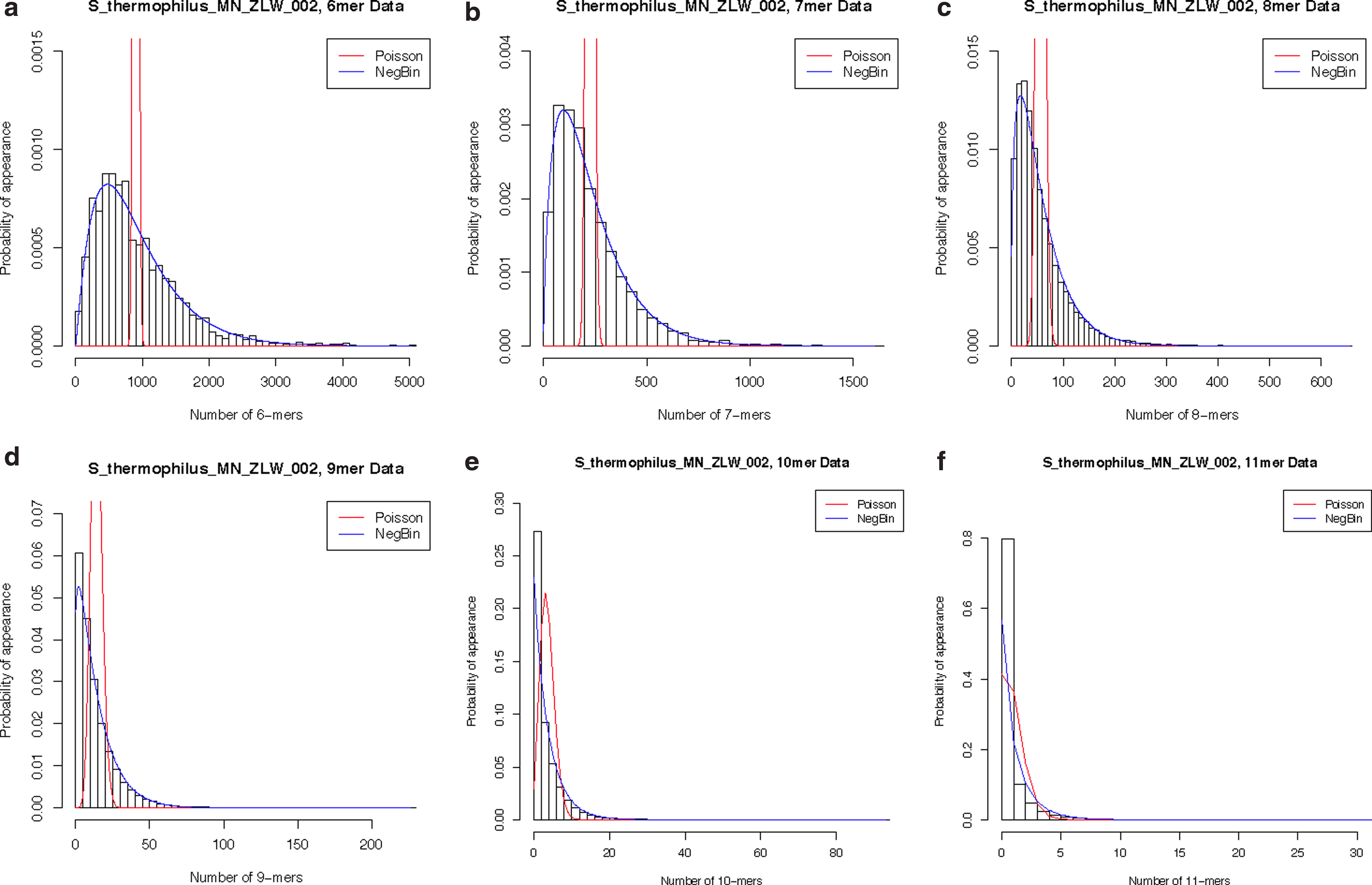
Empirical frequencies. Empirical frequency of S. thermophilus for (a) 6-mers, (b) 7-mers, (c) 8-mers, (d) 9-mers, (e) 10-mers, and (f ) 11-mers. The x-axis describes the abundance of n-mers, and the y-axis describes the probability of appearance with that abundance.

Table 1 shows the distribution of nullomers for each n-mer in the 2,199 genomes considered. The numbers of genomes with nullomers present are 150, 602, and 2,012 in the 6-, 7-, and 8-mers, respectively. All of the 2,199 genomes have nullomers present in the 9-, 10-, and 11-mers, indicating a strong presence of these absent words in these higher order n-mers. The percentage of nullomers in each n-mer is also presented with its corresponding range, where the percentage increases from 0.30 (6-mers) to 49.96 (11-mers). Table 2 shows the AIC results when comparing the various distributions for the n-mers in the 2,199 genomes. More specifically, the table displays the number of times each genome distribution's AIC value was lowest when comparing across the four different models. Overall, the negative binomial distribution has the best fit in all but 8 of the 6-mers, over 98% of the 7-mers, roughly 93% of the 8- and 9-mers, and over 99% of the 10- and 11-mers. There is a small percentage of 9-mers (<7%) and an even smaller percentage of 10-mers (0.73%) and 11-mers (0.09%) where the ZINB has a better fit. The Poisson distribution and its zero-inflated counterpart do not fit this data well across the various n-mers in any of the 2,199 genomes.

Table 1.

Distribution of Nullomers

Nullomers	6-mer	7-mer	8-mer	9-mer	10-mer	11-mer
N (out of 2,199 genomes)	150	602	2,012	2,199	2,199	2,199
Mean (%)	0.30	0.76	1.48	6.28	21.57	49.96
Range (%)	(0.02, 6.27)	(0.01, 27.83)	(0.002, 55.54)	(0.01, 78.31)	(0.90, 91.15)	(12.27, 96.85)

Count (N), mean (%), and range (%) of nullomers for each n-mer in 2,199 genomes.

Table 2.

Summary of Akaike Information Criterion Statistics

	6-mer		7-mer		8-mer		9-mer		10-mer		11-mer
Distribution	Frequency	Percent	Frequency	Percent	Frequency	Percent	Frequency	Percent	Frequency	Percent	Frequency	Percent
NB	2,191	99.64	2,161	98.27	2,046	93.04	2,046	93.04	2,183	99.27	2,197	99.91
ZINB	8	0.36	38	1.73	153	6.96	153	6.96	16	0.73	2	0.09
Poisson	0	0	0	0	0	0	0	0	0	0	0	0
ZIP	0	0	0	0	0	0	0	0	0	0	0	0
Total	2,199	100	2,199	100	2,199	100	2,199	100	2,199	100	2,199	100

Count and percentage of lowest AIC statistic when comparing the Poisson, negative binomial, ZIP, and ZINB distributions for each n-mer in 2,199 genomes. AIC, Akaike information criterion; NB, negative binomial; ZINB, zero-inflated negative binomial; ZIP, zero-inflated Poisson.

4. Conclusions

The purpose of this study was to characterize the distribution of several n-mers in an effort to model prokaryotic genomes with a more flexible and accurate distribution. Initially, we used graphical approaches in determining how to characterize each distribution. Our histograms show that each n-mer has a unimodal distribution with an extreme right tail. The histograms for 9-, 10-, and 11-mers for the randomly chosen genomes all showed a spike at zero, indicating the possibility of an increase in the frequency of nullomers. These absent words create a layer of complexity when describing the distribution of any DNA sequence; therefore, probabilistic models assuming the Poisson distribution may not be the appropriate choice to fully describe the behavior of a given genome.

Moving beyond the graphical approaches, which are more subjective, we chose to use a more objective method, such as the AIC statistic. Using this statistic showed that, for all 2,199 n-mers considered, at least 93% of the genomes preferred the negative binomial distribution, in comparison to the other three distributions. There were a few genomes that preferred the ZINB, but this percentage was small. The Poisson and ZIP distributions were not the best fit in any of the 2,199 genomes considered.

Interestingly, the preference for the ZINB did not increase with n-mer size and, in fact, 7% of the genomes were best fit with the ZINB in the 8- and 9-mer range. Upon further investigation, as shown in Supplementary Data File 5, there were interesting results. For the 9-mers, every Escherichia coli and many of the Salmonella strains have a better fit with the ZINB. For 8-mers, a significant amount of E. coli and Salmonella are better fit with ZINB over the negative binomial, but the correlation is less clear. However, Shigella, which is sometimes treated as a subgenus of E. coli, is best fit with negative binomial at both of these n-mer sizes (i.e., 8 and 9). Such analysis is revealing particular structures that are phylogenetically independent. Another interesting result is that at the 11-mer level, the only genomes that are better fit by the ZINB are the Candidatus Tremblaya genomes, which have the smallest genomes and have a higher noncoding portion (27%) than most prokaryotes (McCutcheon and Moran, 2012). However, this is not the case for the 10-mers. We hypothesized that the modeling is highlighting particular genomes' n-mer usage at different sizes of n and may be related to “coding” structure, in the case of E. coli and Salmonella, and noncoding structure, in the case of Trembalaya. While it is difficult to make concrete biological conclusions from the n-mer distribution modeling, it provides novel opportunities for further analysis into genome structure.

Our study was able to move beyond examining the characteristics of the common Poisson process, which is often used to illustrate the distribution of prokaryotic genomes. Although the Poisson distribution was not preferred in any of the genomes considered, the advantage of having only one parameter to estimate for this distribution remains. If there are excessive zeros present, the ZIP is often used, but its corresponding parameter estimates can be severely biased if the nonzero counts are overdispersed in relation to the Poisson distribution. The negative binomial and ZINB extend the traditional Poisson setting and are more flexible in handling overdispersion that can be caused by an increase in nullomers as well as outliers. Although these models are more complex and contain extra parameters in need of estimation, they tend to have a better model fit than a Poisson distribution. In an effort to characterize the distribution of the frequency of n-mers, researchers should also consider other discrete distributions that are more flexible and adjust for possible overdispersion. Such models can improve prokaryotic sequence classification and provide insights into genome organization.

Footnotes

Acknowledgments

This work was supported by the National Science Foundation Award No. DMS-1120622. All work was initiated when W.Z. and J.H. were affiliated with Drexel University.

Author Disclosure Statement

No competing financial interests exist.

References

Acquisti

, Poste

, Curtiss

, and Kumar

2007. Nullomers: really a matter of natural selection?. PloS ONE, 2, e1022.

Agresti

2002. Categorical Data Analysis (2nd ed.). John Wiley & Sons, Hoboken, NJ.

Akaike

1974. A new look at the statistical model identification. IEEE Trans. Automatic Control, 19, 716–723.

Benson

D.A.

, Karsch-Mizrachi

, Clark

, et al. 2012. GenBank. Nucleic Acids Res., 40, D48–D53.

Burnham

K.P.

, and Anderson

D.R.

2004. Multimodel inference understanding AIC and BIC in model selection. Soc. Methods Res., 33, 261–304.

Casella

, and Berger

R.L.

1990. Statistical Inference (Vol. 70): Duxbury Press, Belmont, CA.

Chen

S.F.

, and Goodman

1996. An empirical study of smoothing techniques for language modeling. Presented at the Proceedings of the 34th Annual Meeting on Association for Computational Linguistics.

Chor

, Horn

, Goldman

, et al. 2009. Genomic DNA k-mer spectra: models and modalities. Genome Biol., 10, R108.

Cohen

A.C.

1963. Estimation in Mixtures of Discrete Distributions. Statistical Pub. Society.

10.

Feller

2008. An Introduction to Probability Theory and Its Applications (Vol. 2). John Wiley & Sons, Hoboken, NJ.

11.

Fofanov

, Luo

, Katili

, et al. 2004. How independent are the appearances of n-mers in different genomes?. Bioinformatics, 20, 2421–2428.

12.

Hampikian

, and Andersen

2006. Absent sequences: nullomers and primes. Presented at the Proceedings of the Pacific Symposium on Biocomputing.

13.

Johnson

N.L.

, and Kotz

1969. Distribution in Statistics: Discrete Distribution: Wiley, New York.

14.

Kidwell

M.G.

2002. Transposable elements and the evolution of genome size in eukaryotes. Genetica, 115, 49–63.

15.

Lambert

1992. Zero-inflated Poisson regression, with an application to defects in manufacturing. Technometrics, 34, 1–14.

16.

McCutcheon

J.P.

, and Moran

N.A.

2012. Extreme genome reduction in symbotic bacteria. Nat. Rev. Microbiol., 10, 13–26.

17.

Mullahy

1986. Specification and testing of some modified count data models. J. Econometrics, 33, 341–365.

18.

R Core Team. 2012. R: A Language and Environment for Statistical Computing. R Foundation for Statistical Computing, Vienna, Austria. Available at: www.R-project.org/

19.

Reinert

, Schbath

, and Waterman

M.S.

2000. Probabilistic and statistical properties of words: an overview. J Comput. Biol., 7, 1–46.

20.

Robin

2002. A compound Poisson model for word occurrences in DNA sequences. J. R. Stat. Soc. C, 51, 437–451.

21.

Robin

, and Schbath

2001. Numerical comparison of several approximations of the word count distribution in random sequences. J. Comput. Biol., 8, 349–359.

22.

Rosen

, Garbarine

, Caseiro

, et al. 2008. Metagenome fragment classification using n-mer frequency profiles. Adv. Bioinformatics, 2008, 205969.

23.

SAS Institute Inc.. 2012. SAS Software, Version 9.3. Cary, NC.

24.

Yau

K.K.W.

, Wang

, and Lee

A.H.

2003. Zero-inflated negative binomial mixed regression modeling of over-dispersed count data with extra zeros. Biometrical J., 45, 437–452.

Supplementary Material

Please find the following supplemental material available below.

For Open Access articles published under a Creative Commons License, all supplemental material carries the same license as the article it is associated with.

For non-Open Access articles published, all supplemental material carries a non-exclusive license, and permission requests for re-use of supplemental material or any part of supplemental material shall be sent directly to the copyright owner as specified in the copyright notice associated with the article.

0.22 MB

1.06 MB

0.00 MB