Bayesian Blind Source Separation for Data with Network Structure

2.1. A stationary Gaussian model

Let G=(V, E) be a directed acyclic graph, with \documentclass{aastex}\usepackage{amsbsy}\usepackage{amsfonts}\usepackage{amssymb}\usepackage{bm}\usepackage{mathrsfs}\usepackage{pifont}\usepackage{stmaryrd}\usepackage{textcomp}\usepackage{portland, xspace}\usepackage{amsmath, amsxtra}\pagestyle{empty}\DeclareMathSizes{10}{9}{7}{6}\begin{document} $$V = \{ v_i \, \mid \, i = 1 , \ldots , N \} $$ \end{document} the set of nodes and \documentclass{aastex}\usepackage{amsbsy}\usepackage{amsfonts}\usepackage{amssymb}\usepackage{bm}\usepackage{mathrsfs}\usepackage{pifont}\usepackage{stmaryrd}\usepackage{textcomp}\usepackage{portland, xspace}\usepackage{amsmath, amsxtra}\pagestyle{empty}\DeclareMathSizes{10}{9}{7}{6}\begin{document} $$E \subset V \times V$$ \end{document} the set of edges. The nodes are ordered in a way such that for each node v_i all parent nodes have indices lower than i. Let \documentclass{aastex}\usepackage{amsbsy}\usepackage{amsfonts}\usepackage{amssymb}\usepackage{bm}\usepackage{mathrsfs}\usepackage{pifont}\usepackage{stmaryrd}\usepackage{textcomp}\usepackage{portland, xspace}\usepackage{amsmath, amsxtra}\pagestyle{empty}\DeclareMathSizes{10}{9}{7}{6}\begin{document} $$pa_i = ( j_1 < \ldots < j_{n_i} )$$ \end{document} index all parent nodes of v_i, and we assume that \documentclass{aastex}\usepackage{amsbsy}\usepackage{amsfonts}\usepackage{amssymb}\usepackage{bm}\usepackage{mathrsfs}\usepackage{pifont}\usepackage{stmaryrd}\usepackage{textcomp}\usepackage{portland, xspace}\usepackage{amsmath, amsxtra}\pagestyle{empty}\DeclareMathSizes{10}{9}{7}{6}\begin{document} $$v_1 , \ldots , v_{n_0 - 1}$$ \end{document} are the root nodes of the graph, that is, \documentclass{aastex}\usepackage{amsbsy}\usepackage{amsfonts}\usepackage{amssymb}\usepackage{bm}\usepackage{mathrsfs}\usepackage{pifont}\usepackage{stmaryrd}\usepackage{textcomp}\usepackage{portland, xspace}\usepackage{amsmath, amsxtra}\pagestyle{empty}\DeclareMathSizes{10}{9}{7}{6}\begin{document} $$pa_i = \emptyset \ { \rm for} \ i < n_0$$ \end{document} .

The associated Bayesian network (Lauritzen, 1996) is then given by a set of random variables \documentclass{aastex}\usepackage{amsbsy}\usepackage{amsfonts}\usepackage{amssymb}\usepackage{bm}\usepackage{mathrsfs}\usepackage{pifont}\usepackage{stmaryrd}\usepackage{textcomp}\usepackage{portland, xspace}\usepackage{amsmath, amsxtra}\pagestyle{empty}\DeclareMathSizes{10}{9}{7}{6}\begin{document} $$\textbf{\textit{S}} = ( \textbf{\textit{s}} ( i ) ) _{i = 1}^N$$ \end{document} such that the joint distribution decomposes as \documentclass{aastex}\usepackage{amsbsy}\usepackage{amsfonts}\usepackage{amssymb}\usepackage{bm}\usepackage{mathrsfs}\usepackage{pifont}\usepackage{stmaryrd}\usepackage{textcomp}\usepackage{portland, xspace}\usepackage{amsmath, amsxtra}\pagestyle{empty}\DeclareMathSizes{10}{9}{7}{6}\begin{document} \begin{align*}{ \rm p} ( \textbf{\textit{S}} ) = \prod_{i = n_0}^N { \rm p} ( \textbf{\textit{s}} ( i ) \, \mid \, { \bf Pa} ( i ) ) \prod_{i = 1}^{n_0 - 1} { \rm p} ( \textbf{\textit{s}} ( i ) ) . \tag{1}\end{align*} \end{document}

Here, \documentclass{aastex}\usepackage{amsbsy}\usepackage{amsfonts}\usepackage{amssymb}\usepackage{bm}\usepackage{mathrsfs}\usepackage{pifont}\usepackage{stmaryrd}\usepackage{textcomp}\usepackage{portland, xspace}\usepackage{amsmath, amsxtra}\pagestyle{empty}\DeclareMathSizes{10}{9}{7}{6}\begin{document} $${ \bf Pa} ( i ) = ( \textbf{\textit{s}} ( j_1 ) ^{ \prime} , \ldots , \textbf{\textit{s}} ( j_{n_i} ) ^{ \prime} ) ^{ \prime}$$ \end{document} with \documentclass{aastex}\usepackage{amsbsy}\usepackage{amsfonts}\usepackage{amssymb}\usepackage{bm}\usepackage{mathrsfs}\usepackage{pifont}\usepackage{stmaryrd}\usepackage{textcomp}\usepackage{portland, xspace}\usepackage{amsmath, amsxtra}\pagestyle{empty}\DeclareMathSizes{10}{9}{7}{6}\begin{document} $$j_1 < \ldots < j_{n_i}$$ \end{document} denotes the vector of all random variables associated with the parent nodes of v_i.

From now we assume Gaussian random variables \documentclass{aastex}\usepackage{amsbsy}\usepackage{amsfonts}\usepackage{amssymb}\usepackage{bm}\usepackage{mathrsfs}\usepackage{pifont}\usepackage{stmaryrd}\usepackage{textcomp}\usepackage{portland, xspace}\usepackage{amsmath, amsxtra}\pagestyle{empty}\DeclareMathSizes{10}{9}{7}{6}\begin{document} $$( \textbf{\textit{s}} ( i ) ) _{i = 1}^N$$ \end{document} with state space \documentclass{aastex}\usepackage{amsbsy}\usepackage{amsfonts}\usepackage{amssymb}\usepackage{bm}\usepackage{mathrsfs}\usepackage{pifont}\usepackage{stmaryrd}\usepackage{textcomp}\usepackage{portland, xspace}\usepackage{amsmath, amsxtra}\pagestyle{empty}\DeclareMathSizes{10}{9}{7}{6}\begin{document} $${\mathbb R}^q$$ \end{document} . We further assign edge weights \documentclass{aastex}\usepackage{amsbsy}\usepackage{amsfonts}\usepackage{amssymb}\usepackage{bm}\usepackage{mathrsfs}\usepackage{pifont}\usepackage{stmaryrd}\usepackage{textcomp}\usepackage{portland, xspace}\usepackage{amsmath, amsxtra}\pagestyle{empty}\DeclareMathSizes{10}{9}{7}{6}\begin{document} $$\lambda_{ij} \in{\mathbb R}$$ \end{document} to all edges \documentclass{aastex}\usepackage{amsbsy}\usepackage{amsfonts}\usepackage{amssymb}\usepackage{bm}\usepackage{mathrsfs}\usepackage{pifont}\usepackage{stmaryrd}\usepackage{textcomp}\usepackage{portland, xspace}\usepackage{amsmath, amsxtra}\pagestyle{empty}\DeclareMathSizes{10}{9}{7}{6}\begin{document} $$e_{ij} \in E$$ \end{document} , and we denote the resulting weighted graph by \documentclass{aastex}\usepackage{amsbsy}\usepackage{amsfonts}\usepackage{amssymb}\usepackage{bm}\usepackage{mathrsfs}\usepackage{pifont}\usepackage{stmaryrd}\usepackage{textcomp}\usepackage{portland, xspace}\usepackage{amsmath, amsxtra}\pagestyle{empty}\DeclareMathSizes{10}{9}{7}{6}\begin{document} $$G_{ \Lambda} = ( V , E , \Lambda )$$ \end{document} . Let s (i) and s (j) be random variables associated with adjacent nodes of the graph. We make the following stationarity (and scaling) assumptions: \documentclass{aastex}\usepackage{amsbsy}\usepackage{amsfonts}\usepackage{amssymb}\usepackage{bm}\usepackage{mathrsfs}\usepackage{pifont}\usepackage{stmaryrd}\usepackage{textcomp}\usepackage{portland, xspace}\usepackage{amsmath, amsxtra}\pagestyle{empty}\DeclareMathSizes{10}{9}{7}{6}\begin{document} \begin{align*} & ( { \rm A}1 ) \ {\mathbb E} [ \textbf{\textit{s}} ( i ) ] = 0_q , \\ & ( { \rm A}2 ) \ { \rm Cov} ( \textbf{\textit{s}} ( i ) , \textbf{\textit{s}} ( i ) ) = I_q , \\ & ( { \rm A}3 ) \ { \rm Cov} ( \textbf{\textit{s}} ( i ) , \textbf{\textit{s}} ( j ) ) = \lambda_{ij}D.\end{align*} \end{document}

The parameter D is constant over the network, and we call it the graph-delayed covariance of the stationary Gaussian model. According to our actual purpose of source separation, we assume that \documentclass{aastex}\usepackage{amsbsy}\usepackage{amsfonts}\usepackage{amssymb}\usepackage{bm}\usepackage{mathrsfs}\usepackage{pifont}\usepackage{stmaryrd}\usepackage{textcomp}\usepackage{portland, xspace}\usepackage{amsmath, amsxtra}\pagestyle{empty}\DeclareMathSizes{10}{9}{7}{6}\begin{document} $$D = { \rm diag} ( d_1 , \ldots , d_q )$$ \end{document} is a diagonal matrix. The larger an entry d_i the larger is the (absolute) value of the covariance between two adjacent random variables in the ith component.

With (A1)–(A3) and the decomposition of p( S ) in Equation (1), all conditional distributions are uniquely defined, and we get \documentclass{aastex}\usepackage{amsbsy}\usepackage{amsfonts}\usepackage{amssymb}\usepackage{bm}\usepackage{mathrsfs}\usepackage{pifont}\usepackage{stmaryrd}\usepackage{textcomp}\usepackage{portland, xspace}\usepackage{amsmath, amsxtra}\pagestyle{empty}\DeclareMathSizes{10}{9}{7}{6}\begin{document} \begin{align*}\textbf{\textit{s}} ( i ) \,\mid\, {\bf Pa} ( i ) \,\sim \,\begin{cases}{\cal N} ( 0_q , I_q ) \qquad \qquad \qquad \quad if \ {\bf Pa}( i ) = \emptyset , \\ { \cal N} ( \omega_D ( i ) { \bf Pa} ( i ) , \Sigma_D ( i ) ) \qquad\, otherwise , \end{cases} \tag{2}\end{align*} \end{document}

where \documentclass{aastex}\usepackage{amsbsy}\usepackage{amsfonts}\usepackage{amssymb}\usepackage{bm}\usepackage{mathrsfs}\usepackage{pifont}\usepackage{stmaryrd}\usepackage{textcomp}\usepackage{portland, xspace}\usepackage{amsmath, amsxtra}\pagestyle{empty}\DeclareMathSizes{10}{9}{7}{6}\begin{document} $$\omega_D ( i ) \in {\mathbb R}^{q \times q \ n_i}$$ \end{document} and \documentclass{aastex}\usepackage{amsbsy}\usepackage{amsfonts}\usepackage{amssymb}\usepackage{bm}\usepackage{mathrsfs}\usepackage{pifont}\usepackage{stmaryrd}\usepackage{textcomp}\usepackage{portland, xspace}\usepackage{amsmath, amsxtra}\pagestyle{empty}\DeclareMathSizes{10}{9}{7}{6}\begin{document} $$\Sigma_D ( i ) \in {\mathbb R}^{q \times q}$$ \end{document} depend only on the graph-delayed covariance D. If D is diagonal we have that Σ _D (i) is also diagonal and ω_D (i) consists of blocks of diagonal matrices. Dependent on the weighted graph G_Λ one can determine an interval \documentclass{aastex}\usepackage{amsbsy}\usepackage{amsfonts}\usepackage{amssymb}\usepackage{bm}\usepackage{mathrsfs}\usepackage{pifont}\usepackage{stmaryrd}\usepackage{textcomp}\usepackage{portland, xspace}\usepackage{amsmath, amsxtra}\pagestyle{empty}\DeclareMathSizes{10}{9}{7}{6}\begin{document} $$I^G \subseteq {\mathbb R}$$ \end{document} such that all covariance matrices Σ _D (i) are positive definite for diagonal D with components in I^G. We refer to the Gaussian distribution p( S ) defined (1) in Equations and (2) as source model \documentclass{aastex}\usepackage{amsbsy}\usepackage{amsfonts}\usepackage{amssymb}\usepackage{bm}\usepackage{mathrsfs}\usepackage{pifont}\usepackage{stmaryrd}\usepackage{textcomp}\usepackage{portland, xspace}\usepackage{amsmath, amsxtra}\pagestyle{empty}\DeclareMathSizes{10}{9}{7}{6}\begin{document} $${ \cal M} ( G_{ \Lambda} , q )$$ \end{document} , where q is the dimension of the random variables. The distribution is parameterized by the graph-delayed covariance D, and if samples from \documentclass{aastex}\usepackage{amsbsy}\usepackage{amsfonts}\usepackage{amssymb}\usepackage{bm}\usepackage{mathrsfs}\usepackage{pifont}\usepackage{stmaryrd}\usepackage{textcomp}\usepackage{portland, xspace}\usepackage{amsmath, amsxtra}\pagestyle{empty}\DeclareMathSizes{10}{9}{7}{6}\begin{document} $${ \cal M} ( G_{ \Lambda} , q )$$ \end{document} are given, the maximum likelihood approach naturally yields an estimate \documentclass{aastex}\usepackage{amsbsy}\usepackage{amsfonts}\usepackage{amssymb}\usepackage{bm}\usepackage{mathrsfs}\usepackage{pifont}\usepackage{stmaryrd}\usepackage{textcomp}\usepackage{portland, xspace}\usepackage{amsmath, amsxtra}\pagestyle{empty}\DeclareMathSizes{10}{9}{7}{6}\begin{document} $${\hat D}^{ \rm ML}$$ \end{document} .

The concept of a graph-delayed covariance was originally introduced by Kowarsch et al. (2010). We now shortly review their definition. For a weighted directed graph \documentclass{aastex}\usepackage{amsbsy}\usepackage{amsfonts}\usepackage{amssymb}\usepackage{bm}\usepackage{mathrsfs}\usepackage{pifont}\usepackage{stmaryrd}\usepackage{textcomp}\usepackage{portland, xspace}\usepackage{amsmath, amsxtra}\pagestyle{empty}\DeclareMathSizes{10}{9}{7}{6}\begin{document} $$G_{ \cal K} = ( V , E , { \cal K} )$$ \end{document} with weights \documentclass{aastex}\usepackage{amsbsy}\usepackage{amsfonts}\usepackage{amssymb}\usepackage{bm}\usepackage{mathrsfs}\usepackage{pifont}\usepackage{stmaryrd}\usepackage{textcomp}\usepackage{portland, xspace}\usepackage{amsmath, amsxtra}\pagestyle{empty}\DeclareMathSizes{10}{9}{7}{6}\begin{document} $$\kappa_{ij} \in {\mathbb R}$$ \end{document} and associated random variables \documentclass{aastex}\usepackage{amsbsy}\usepackage{amsfonts}\usepackage{amssymb}\usepackage{bm}\usepackage{mathrsfs}\usepackage{pifont}\usepackage{stmaryrd}\usepackage{textcomp}\usepackage{portland, xspace}\usepackage{amsmath, amsxtra}\pagestyle{empty}\DeclareMathSizes{10}{9}{7}{6}\begin{document} $$\textbf{\textit{S}} = \left( \textbf{\textit{s}} ( i ) \right) _{i = 1}^N$$ \end{document} , they considered the covariance between a node and the weighted sum of its parent nodes as \documentclass{aastex}\usepackage{amsbsy}\usepackage{amsfonts}\usepackage{amssymb}\usepackage{bm}\usepackage{mathrsfs}\usepackage{pifont}\usepackage{stmaryrd}\usepackage{textcomp}\usepackage{portland, xspace}\usepackage{amsmath, amsxtra}\pagestyle{empty}\DeclareMathSizes{10}{9}{7}{6}\begin{document} \begin{align*}D^{ \rm Pa} = { \rm Cov} \left( \sum_{i \in pa_j} \kappa_{ij} \textbf{\textit{s}} ( i ) , \textbf{\textit{s}} ( j ) \right) , \tag{3}\end{align*} \end{document}

and they assumed that it is independent of the index j. For \documentclass{aastex}\usepackage{amsbsy}\usepackage{amsfonts}\usepackage{amssymb}\usepackage{bm}\usepackage{mathrsfs}\usepackage{pifont}\usepackage{stmaryrd}\usepackage{textcomp}\usepackage{portland, xspace}\usepackage{amsmath, amsxtra}\pagestyle{empty}\DeclareMathSizes{10}{9}{7}{6}\begin{document} $$\kappa_{ij} = ( \mid { \bf Pa} ( j ) \mid \lambda_{ij} ) ^{ - 1}$$ \end{document} with λ _ij from above we have D^Pa=D, where D is the graph-delayed covariance in the stationary Gaussian model. To estimate D^Pa from samples \documentclass{aastex}\usepackage{amsbsy}\usepackage{amsfonts}\usepackage{amssymb}\usepackage{bm}\usepackage{mathrsfs}\usepackage{pifont}\usepackage{stmaryrd}\usepackage{textcomp}\usepackage{portland, xspace}\usepackage{amsmath, amsxtra}\pagestyle{empty}\DeclareMathSizes{10}{9}{7}{6}\begin{document} $$s ( 1 ) , \ldots , s ( N )$$ \end{document} they introduced \documentclass{aastex}\usepackage{amsbsy}\usepackage{amsfonts}\usepackage{amssymb}\usepackage{bm}\usepackage{mathrsfs}\usepackage{pifont}\usepackage{stmaryrd}\usepackage{textcomp}\usepackage{portland, xspace}\usepackage{amsmath, amsxtra}\pagestyle{empty}\DeclareMathSizes{10}{9}{7}{6}\begin{document} \begin{align*}\hat { D } ^ { \rm Pa } = \frac { 1 } { N - n_0 - 1 } \sum_ { j = n_0 } ^N \sum_ { i \in pa_j } \kappa_ { ij } s ( i ) \ s ( j ) ^ { \prime } , \tag { 4 } \end{align*} \end{document}

where \documentclass{aastex}\usepackage{amsbsy}\usepackage{amsfonts}\usepackage{amssymb}\usepackage{bm}\usepackage{mathrsfs}\usepackage{pifont}\usepackage{stmaryrd}\usepackage{textcomp}\usepackage{portland, xspace}\usepackage{amsmath, amsxtra}\pagestyle{empty}\DeclareMathSizes{10}{9}{7}{6}\begin{document} $$n_0 , \ldots , N$$ \end{document} are all indices of nonroot nodes. According to assumption (A3), we actually have more detailed information about the covariance between adjacent variables. We therefore additionally consider the following refined edge-based estimate: \documentclass{aastex}\usepackage{amsbsy}\usepackage{amsfonts}\usepackage{amssymb}\usepackage{bm}\usepackage{mathrsfs}\usepackage{pifont}\usepackage{stmaryrd}\usepackage{textcomp}\usepackage{portland, xspace}\usepackage{amsmath, amsxtra}\pagestyle{empty}\DeclareMathSizes{10}{9}{7}{6}\begin{document} \begin{align*}\hat D^ { \rm E } = \frac { 1 } { \mid E \mid - 1 } \sum_ { ( i , j ) \in E } \frac { 1 } { \lambda_ { ij } } s ( i ) \ s ( j ) ^ { \prime } . \tag { 5 } \end{align*} \end{document}

Both estimates \documentclass{aastex}\usepackage{amsbsy}\usepackage{amsfonts}\usepackage{amssymb}\usepackage{bm}\usepackage{mathrsfs}\usepackage{pifont}\usepackage{stmaryrd}\usepackage{textcomp}\usepackage{portland, xspace}\usepackage{amsmath, amsxtra}\pagestyle{empty}\DeclareMathSizes{10}{9}{7}{6}\begin{document} $$\hat D^{ \rm Pa}$$ \end{document} and \documentclass{aastex}\usepackage{amsbsy}\usepackage{amsfonts}\usepackage{amssymb}\usepackage{bm}\usepackage{mathrsfs}\usepackage{pifont}\usepackage{stmaryrd}\usepackage{textcomp}\usepackage{portland, xspace}\usepackage{amsmath, amsxtra}\pagestyle{empty}\DeclareMathSizes{10}{9}{7}{6}\begin{document} $$\hat D^{ \rm E}$$ \end{document} yield nonprobabilistic algorithms to separate network data—Grade(Pa) and Grade(E). The former is the original method from Kowarsch et al. (2010), and in section 4.2 we shortly introduce both algorithms for estimation comparison.

2.2. Graph models for simulations

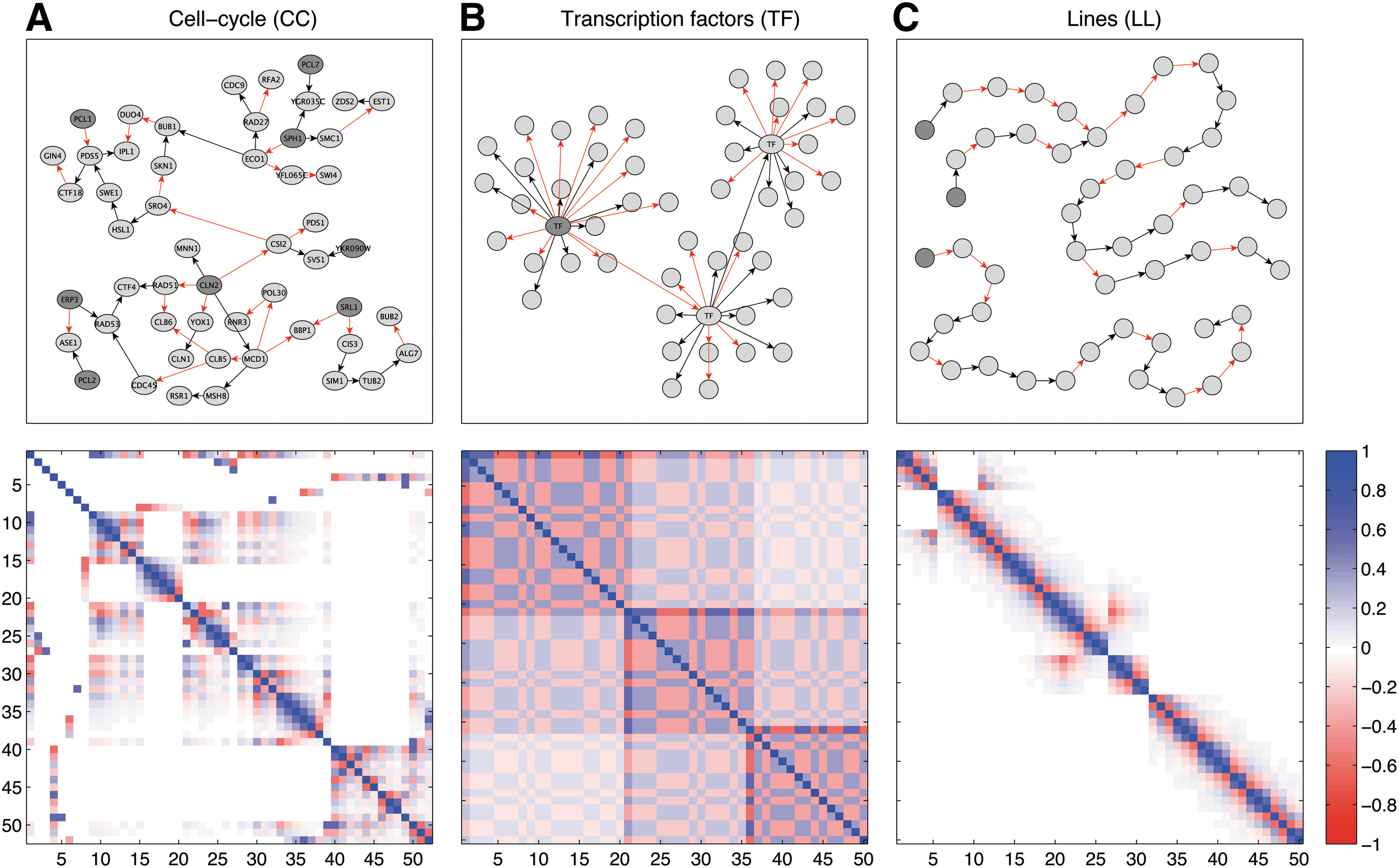
To illustrate the covariance structure of the stationary Gaussian model we introduce three graph models. All graphs are related to biological networks, or to time-series for comparison. In section 4 we again consider these graph models in our simulations about source separation.

(CC) Cell-cycle: The estimated network for the cell-cycle pathway based on gene expression data (Imoto et al., 2002). The network consists of 81 nodes and 84 edges.

(TF) Transcription factors: Three hub nodes and each directly signals on a subset of nodes.

(LL) Line signals: Similar to time-series, we define a network that consists of two line signals sharing the middle part, and one separated line signal.

Figure 1 illustrates these networks together with the associated covariance structure, and we randomly assigned weights ±1 to the edges. Note that one can theoretically consider any weights \documentclass{aastex}\usepackage{amsbsy}\usepackage{amsfonts}\usepackage{amssymb}\usepackage{bm}\usepackage{mathrsfs}\usepackage{pifont}\usepackage{stmaryrd}\usepackage{textcomp}\usepackage{portland, xspace}\usepackage{amsmath, amsxtra}\pagestyle{empty}\DeclareMathSizes{10}{9}{7}{6}\begin{document} $$\lambda_{ij} \in {\mathbb R}$$ \end{document} .

OPEN IN VIEWER

FIG. 1.

Graph models and covariance structure. The upper graphics illustrate a connected subnetwork of cell-cycle (CC), transcription factors (TF), and lines (LL). Darker nodes indicate root nodes, and we randomly assigned edge weights with values +1 (black) and −1 (red). The lower graphics show the covariance structure associated with each graph model for one-dimensional random variables. The graph-delayed covariance was set to D = 0.6.

3. A Blind Source Separation Model for Mixed Network Data

In blind source separation (BSS) we assume that we observe a linear mixture of the actual signals of interest. The aim is to estimate the mixing as well as the underlying signals. In the following we derive a new blind source separation method for network data and decribe the unobserved (latent) signals in terms of the source model from the last section.

3.1. Linear Mixing Model

We consider the following mixing model: \documentclass{aastex}\usepackage{amsbsy}\usepackage{amsfonts}\usepackage{amssymb}\usepackage{bm}\usepackage{mathrsfs}\usepackage{pifont}\usepackage{stmaryrd}\usepackage{textcomp}\usepackage{portland, xspace}\usepackage{amsmath, amsxtra}\pagestyle{empty}\DeclareMathSizes{10}{9}{7}{6}\begin{document} $$\textbf{\textit{X}} = \left( \textbf{\textit{x}} ( i ) \right)_{i = 1}^{N}$$ \end{document} are observed Gaussian variables with state space \documentclass{aastex}\usepackage{amsbsy}\usepackage{amsfonts}\usepackage{amssymb}\usepackage{bm}\usepackage{mathrsfs}\usepackage{pifont}\usepackage{stmaryrd}\usepackage{textcomp}\usepackage{portland, xspace}\usepackage{amsmath, amsxtra}\pagestyle{empty}\DeclareMathSizes{10}{9}{7}{6}\begin{document} $${\mathbb R}^{m}$$ \end{document} , and we assume latent Gaussian variables \documentclass{aastex}\usepackage{amsbsy}\usepackage{amsfonts}\usepackage{amssymb}\usepackage{bm}\usepackage{mathrsfs}\usepackage{pifont}\usepackage{stmaryrd}\usepackage{textcomp}\usepackage{portland, xspace}\usepackage{amsmath, amsxtra}\pagestyle{empty}\DeclareMathSizes{10}{9}{7}{6}\begin{document} $$\textbf{\textit{S}} = \left( \textbf{\textit{s}} ( i ) \right)_{i = 1}^{N}$$ \end{document} with state space \documentclass{aastex}\usepackage{amsbsy}\usepackage{amsfonts}\usepackage{amssymb}\usepackage{bm}\usepackage{mathrsfs}\usepackage{pifont}\usepackage{stmaryrd}\usepackage{textcomp}\usepackage{portland, xspace}\usepackage{amsmath, amsxtra}\pagestyle{empty}\DeclareMathSizes{10}{9}{7}{6}\begin{document} $${\mathbb R}^{q} ( q \leq m )$$ \end{document} , such that each variable x (i) is a linear mixture of the components of the latent variable s (i): \documentclass{aastex}\usepackage{amsbsy}\usepackage{amsfonts}\usepackage{amssymb}\usepackage{bm}\usepackage{mathrsfs}\usepackage{pifont}\usepackage{stmaryrd}\usepackage{textcomp}\usepackage{portland, xspace}\usepackage{amsmath, amsxtra}\pagestyle{empty}\DeclareMathSizes{10}{9}{7}{6}\begin{document} \begin{align*}\textbf{\textit{x}} ( i ) = A \ \textbf{\textit{s}} ( i ) + \mu + \varepsilon ( i ) , \quad i = 1 , \ldots , N. \tag{6}\end{align*} \end{document}

Here, \documentclass{aastex}\usepackage{amsbsy}\usepackage{amsfonts}\usepackage{amssymb}\usepackage{bm}\usepackage{mathrsfs}\usepackage{pifont}\usepackage{stmaryrd}\usepackage{textcomp}\usepackage{portland, xspace}\usepackage{amsmath, amsxtra}\pagestyle{empty}\DeclareMathSizes{10}{9}{7}{6}\begin{document} $$\varepsilon ( i )$$ \end{document} is additive noise distributed as \documentclass{aastex}\usepackage{amsbsy}\usepackage{amsfonts}\usepackage{amssymb}\usepackage{bm}\usepackage{mathrsfs}\usepackage{pifont}\usepackage{stmaryrd}\usepackage{textcomp}\usepackage{portland, xspace}\usepackage{amsmath, amsxtra}\pagestyle{empty}\DeclareMathSizes{10}{9}{7}{6}\begin{document} $$\varepsilon ( i ) \ \sim \ { \cal N} ( 0 , \sigma^2 I_m )$$ \end{document} and independent of the latent variables. \documentclass{aastex}\usepackage{amsbsy}\usepackage{amsfonts}\usepackage{amssymb}\usepackage{bm}\usepackage{mathrsfs}\usepackage{pifont}\usepackage{stmaryrd}\usepackage{textcomp}\usepackage{portland, xspace}\usepackage{amsmath, amsxtra}\pagestyle{empty}\DeclareMathSizes{10}{9}{7}{6}\begin{document} $$A \in {\mathbb R}^{m \times q}$$ \end{document} denotes the mixing matrix and \documentclass{aastex}\usepackage{amsbsy}\usepackage{amsfonts}\usepackage{amssymb}\usepackage{bm}\usepackage{mathrsfs}\usepackage{pifont}\usepackage{stmaryrd}\usepackage{textcomp}\usepackage{portland, xspace}\usepackage{amsmath, amsxtra}\pagestyle{empty}\DeclareMathSizes{10}{9}{7}{6}\begin{document} $$\mu \in {\mathbb R}^m$$ \end{document} is a constant mean vector for all x (i). We refer to the components of the latent variables as sources, that is, for \documentclass{aastex}\usepackage{amsbsy}\usepackage{amsfonts}\usepackage{amssymb}\usepackage{bm}\usepackage{mathrsfs}\usepackage{pifont}\usepackage{stmaryrd}\usepackage{textcomp}\usepackage{portland, xspace}\usepackage{amsmath, amsxtra}\pagestyle{empty}\DeclareMathSizes{10}{9}{7}{6}\begin{document} $$k = 1 , \ldots , q$$ \end{document} we have a source \documentclass{aastex}\usepackage{amsbsy}\usepackage{amsfonts}\usepackage{amssymb}\usepackage{bm}\usepackage{mathrsfs}\usepackage{pifont}\usepackage{stmaryrd}\usepackage{textcomp}\usepackage{portland, xspace}\usepackage{amsmath, amsxtra}\pagestyle{empty}\DeclareMathSizes{10}{9}{7}{6}\begin{document} $$\textbf{\textit{s}}_{k} = \left( \textbf{\textit{s}}_{k} ( i ) \right)_{i = 1}^{N}$$ \end{document} .

We now extend the Bayesian network from section 2.1. Let S be latent variables, and the dependence is given by a weighted graph \documentclass{aastex}\usepackage{amsbsy}\usepackage{amsfonts}\usepackage{amssymb}\usepackage{bm}\usepackage{mathrsfs}\usepackage{pifont}\usepackage{stmaryrd}\usepackage{textcomp}\usepackage{portland, xspace}\usepackage{amsmath, amsxtra}\pagestyle{empty}\DeclareMathSizes{10}{9}{7}{6}\begin{document} $$G_{ \Lambda} = ( V , E , \Lambda )$$ \end{document} as before. We additionally introduce observed variables X , where \documentclass{aastex}\usepackage{amsbsy}\usepackage{amsfonts}\usepackage{amssymb}\usepackage{bm}\usepackage{mathrsfs}\usepackage{pifont}\usepackage{stmaryrd}\usepackage{textcomp}\usepackage{portland, xspace}\usepackage{amsmath, amsxtra}\pagestyle{empty}\DeclareMathSizes{10}{9}{7}{6}\begin{document} $$\textbf{\textit{x}} ( i ) = A \textbf{\textit{s}} ( i ) + \mu + \varepsilon ( i )$$ \end{document} for all i. The joint distribution of X and S then decomposes as \documentclass{aastex}\usepackage{amsbsy}\usepackage{amsfonts}\usepackage{amssymb}\usepackage{bm}\usepackage{mathrsfs}\usepackage{pifont}\usepackage{stmaryrd}\usepackage{textcomp}\usepackage{portland, xspace}\usepackage{amsmath, amsxtra}\pagestyle{empty}\DeclareMathSizes{10}{9}{7}{6}\begin{document} \begin{align*}{\rm p} ( \textbf{\textit{X}} , \textbf{\textit{S}} ) = \prod_{i = 1}^N { \rm p} ( \textbf{\textit{x}} ( i ) \, \mid \, \textbf{\textit{s}} ( i ) ) \prod_{i = n_0}^N { \rm p} ( \textbf{\textit{s}} ( i ) \, \mid \, { \bf Pa} ( i ) ) \prod_{i = 1}^{n_0 - 1}{ \rm p} ( \textbf{\textit{s}} ( i ) ) , \tag{7}\end{align*} \end{document}

where \documentclass{aastex}\usepackage{amsbsy}\usepackage{amsfonts}\usepackage{amssymb}\usepackage{bm}\usepackage{mathrsfs}\usepackage{pifont}\usepackage{stmaryrd}\usepackage{textcomp}\usepackage{portland, xspace}\usepackage{amsmath, amsxtra}\pagestyle{empty}\DeclareMathSizes{10}{9}{7}{6}\begin{document} $$\textbf{\textit{x}} ( i ) \, \mid \, \textbf{\textit{s}} ( i ) \ \sim \ { \cal N} ( A\textbf{\textit{s}} ( i ) + \mu , \sigma^2 I_m )$$ \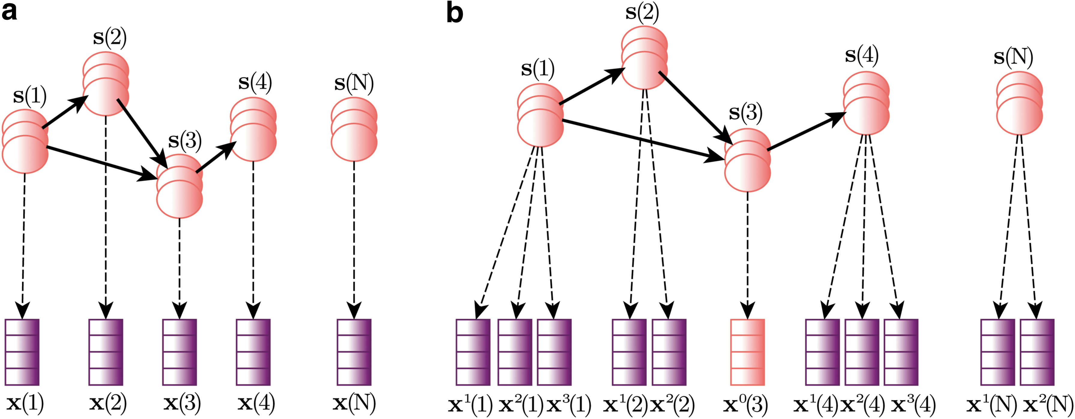end{document} directly follows from the linear mixing. A graphical representation of this latent variable model is given in Figure 2a.

OPEN IN VIEWER

FIG. 2.

Graphical representation of emGrade. Panel (a) shows the basic model with one observed variable x (i)=A s (i)+μ+ɛ(i) for all indices i. In Panel (b) we take into account multiple and/or missing observations. For all indices i we either have multiple observed variables x ^r (i) = A s (i)+μ+ɛ^r (i) with \documentclass{aastex}\usepackage{amsbsy}\usepackage{amsfonts}\usepackage{amssymb}\usepackage{bm}\usepackage{mathrsfs}\usepackage{pifont}\usepackage{stmaryrd}\usepackage{textcomp}\usepackage{portland, xspace}\usepackage{amsmath, amsxtra}\pagestyle{empty}\DeclareMathSizes{10}{9}{7}{6}\begin{document} $$r = 1 , \ldots , r_i$$ \end{document} , or a latent variable x ⁰(i) = A s (i)+μ+ɛ⁰(i) when the observation for index i is missing. In both figures the observed part is shown in purple and the latent part in red.

3.2. Parameter inference using expectation maximization

The unknown components of our model are the parameters θ=(A, μ, σ, D) and the latent variables S , and we are interested in both. A widely used approach for latent variable models is expectation maximization (McLachlan and Krishnan, 2007); that is, parameters and latent variables are updated alternately and each update improves the data log-likelihood \documentclass{aastex}\usepackage{amsbsy}\usepackage{amsfonts}\usepackage{amssymb}\usepackage{bm}\usepackage{mathrsfs}\usepackage{pifont}\usepackage{stmaryrd}\usepackage{textcomp}\usepackage{portland, xspace}\usepackage{amsmath, amsxtra}\pagestyle{empty}\DeclareMathSizes{10}{9}{7}{6}\begin{document} $$\ell ( \theta; \ \textbf{\textit{X}} ) = \ln { \rm p} ( \textbf{\textit{X}} \,\mid \,\theta )$$ \end{document} .

For expectation maximization we need to consider the complete data log-likelihood \documentclass{aastex}\usepackage{amsbsy}\usepackage{amsfonts}\usepackage{amssymb}\usepackage{bm}\usepackage{mathrsfs}\usepackage{pifont}\usepackage{stmaryrd}\usepackage{textcomp}\usepackage{portland, xspace}\usepackage{amsmath, amsxtra}\pagestyle{empty}\DeclareMathSizes{10}{9}{7}{6}\begin{document} $$\ell_c ( \theta; \ \textbf{\textit{X}} , \textbf{\textit{S}} ) = \ln { \rm p} ( \textbf{\textit{X}} , \textbf{\textit{S}} \,\mid \, \theta )$$ \end{document} . Let \documentclass{aastex}\usepackage{amsbsy}\usepackage{amsfonts}\usepackage{amssymb}\usepackage{bm}\usepackage{mathrsfs}\usepackage{pifont}\usepackage{stmaryrd}\usepackage{textcomp}\usepackage{portland, xspace}\usepackage{amsmath, amsxtra}\pagestyle{empty}\DeclareMathSizes{10}{9}{7}{6}\begin{document} $${\mathbb E}_{S \mid X , \theta} [ . ]$$ \end{document} denote the expectation with respect to the posterior distribution S  |  X , θ of the latent variables S given the observable variables X and parameters θ. The expectation of the complete data log-likelihood is then given by \documentclass{aastex}\usepackage{amsbsy}\usepackage{amsfonts}\usepackage{amssymb}\usepackage{bm}\usepackage{mathrsfs}\usepackage{pifont}\usepackage{stmaryrd}\usepackage{textcomp}\usepackage{portland, xspace}\usepackage{amsmath, amsxtra}\pagestyle{empty}\DeclareMathSizes{10}{9}{7}{6}\begin{document} \begin{align*}{\mathbb E}_{S \mid X , \theta} [ \ln { \rm p} ( \textbf{\textit{X}} , \textbf{\textit{S}} \mid \theta ) ] = {\mathbb E}_{S \mid X , \theta} [ \ln { \rm p} ( \textbf{\textit{X}} \mid\textbf{\textit{S}} , A , \mu , \sigma^2 ) ] + {\mathbb E}_{S \mid X , \theta} [ \ln { \rm p} ( \textbf{\textit{S}} \mid D ) ] . \tag{8}\end{align*} \end{document}

For better readability we use the notations A_μ=(A, μ) and s _*(i)=( s (i)′,1)′—both enlarged by a constant component. We then have: \documentclass{aastex}\usepackage{amsbsy}\usepackage{amsfonts}\usepackage{amssymb}\usepackage{bm}\usepackage{mathrsfs}\usepackage{pifont}\usepackage{stmaryrd}\usepackage{textcomp}\usepackage{portland, xspace}\usepackage{amsmath, amsxtra}\pagestyle{empty}\DeclareMathSizes{10}{9}{7}{6}\begin{document} \begin{align*} { \mathbb E } _ { S \mid X , \theta } [ \ln { \rm p } ( \textbf{\textit{X}}\mid\textbf{\textit{S}} , A , \mu , \sigma^2 ) ] = & - \frac { Nm } { 2 } \ln ( 2 \pi ) - \frac { Nm } { 2 } \ln ( \sigma^2 ) \\ & - \frac { 1 } { 2 \sigma^2 } \sum_ { i = 1 } ^N [ { \rm Tr } ( { \mathbb E } _ { S \mid X , \theta } [ \textbf{\textit{x}}(i)\textbf{\textit{x}}(i) ^ { \prime } ] ) \\ & - 2 { \rm Tr } \,( { \mathbb E } _ { S \mid X , \theta } [ \textbf{\textit{s}}_*(i)\textbf{\textit{x}}(i) ^ { \prime } ] A_ \mu ) \\ & + { \rm Tr } \,( { \mathbb E } _ { S \mid X , \theta } [ \textbf{\textit{s}}_*(i)\textbf{\textit{s}}_*(i) ^ { \prime } ] A_ \mu^ { \prime } A_ \mu ) ] \tag{9} \end{align*} \end{document} \documentclass{aastex}\usepackage{amsbsy}\usepackage{amsfonts}\usepackage{amssymb}\usepackage{bm}\usepackage{mathrsfs}\usepackage{pifont}\usepackage{stmaryrd}\usepackage{textcomp}\usepackage{portland, xspace}\usepackage{amsmath, amsxtra}\pagestyle{empty}\DeclareMathSizes{10}{9}{7}{6}\begin{document} \begin{align*} { \mathbb E } _ { S \mid X , \theta } [ { \ln { \rm p } ( \textbf{\textit{S}}\mid D)} = & - \frac { Nq } { 2 } \ln ( 2 \pi ) - \sum_ { i = n_0 } ^N \ln ( { \rm det } ( \Sigma_D ( i ) ) ) \\ & - \frac { 1 } { 2 } \sum_ { i = n_0 } ^N [ { \rm Tr } \, ( { \mathbb E } _ { S \mid X , \theta } [ \textbf{\textit{s}}(i)\textbf{\textit{s}}(i) ^ { \prime } ] \Sigma_D ( i ) ^ { - 1 } ) \\ & - 2 { \rm Tr } \, ( { \mathbb E } _ { S \mid X , \theta } [ \textbf{\textit{s}}(i){ \bf Pa } ( i ) ^ { \prime } ] \Sigma_D ( i ) ^ { - 1 } \omega_D ( i ) ) \\ & + { \rm Tr } \, ( { \mathbb E } _ { S \mid X , \theta } [ { \bf Pa } ( i ) { \bf Pa } ( i ) ^ { \prime } ] \omega_D ( i ) ^ { \prime } \Sigma_D ( i ) ^ { - 1 } \omega_D ( i ) ) ] \\ & - \frac { 1 } { 2 } \sum_ { i = 1 } ^ { n_0 - 1 } { \mathbb E } _ { S \mid X , \theta } [ \textbf{\textit{s}}(i)\textbf{\textit{s}}(i) ^ { \prime } ] \tag {10} \end{align*} \end{document}

The EM-algorithm consists of two steps that are repeated alternately until convergence. In the E-step, we determine the posterior distribution of the latent variables which yields the expectations in (9) and (10). Here, we use the well-known property \documentclass{aastex}\usepackage{amsbsy}\usepackage{amsfonts}\usepackage{amssymb}\usepackage{bm}\usepackage{mathrsfs}\usepackage{pifont}\usepackage{stmaryrd}\usepackage{textcomp}\usepackage{portland, xspace}\usepackage{amsmath, amsxtra}\pagestyle{empty}\DeclareMathSizes{10}{9}{7}{6}\begin{document} $${\mathbb E} [ \textbf{\textit{z}}_1 \textbf{\textit{z}}_2^{ \prime} ] = { \rm Cov} ( \textbf{\textit{z}}_1 , \textbf{\textit{z}}_2 ) + {\mathbb E} [ \textbf{\textit{z}}_1 ] {\mathbb E} [ \textbf{\textit{z}}_2 ] ^{ \prime}$$ \end{document} for random variables z₁ and z₂. If z ₂ or both variables are observed, the l.h.s. equals \documentclass{aastex}\usepackage{amsbsy}\usepackage{amsfonts}\usepackage{amssymb}\usepackage{bm}\usepackage{mathrsfs}\usepackage{pifont}\usepackage{stmaryrd}\usepackage{textcomp}\usepackage{portland, xspace}\usepackage{amsmath, amsxtra}\pagestyle{empty}\DeclareMathSizes{10}{9}{7}{6}\begin{document} $${\mathbb E} [ \textbf{\textit{z}}_1 ] \textbf{\textit{z}}_2^{ \prime}$$ \end{document} and \documentclass{aastex}\usepackage{amsbsy}\usepackage{amsfonts}\usepackage{amssymb}\usepackage{bm}\usepackage{mathrsfs}\usepackage{pifont}\usepackage{stmaryrd}\usepackage{textcomp}\usepackage{portland, xspace}\usepackage{amsmath, amsxtra}\pagestyle{empty}\DeclareMathSizes{10}{9}{7}{6}\begin{document} $$\textbf{\textit{z}}_1 \textbf{\textit{z}}_2^{ \prime}$$ \end{document} , respectively. To get these posterior estimates we use the junction tree algorithm implemented in the Bayes net toolbox for Matlab (Murphy et al., 2001). In the M-step, we maximize \documentclass{aastex}\usepackage{amsbsy}\usepackage{amsfonts}\usepackage{amssymb}\usepackage{bm}\usepackage{mathrsfs}\usepackage{pifont}\usepackage{stmaryrd}\usepackage{textcomp}\usepackage{portland, xspace}\usepackage{amsmath, amsxtra}\pagestyle{empty}\DeclareMathSizes{10}{9}{7}{6}\begin{document} $${\mathbb E}_{S \mid X , \theta} [ \ln { \rm p} ( \textbf{\textit{X}} , \textbf{\textit{S}} ) ]$$ \end{document} with respect to the parameters. Due to our specific stationarity assumptions the toolbox is not applicable for parameter maximization. Let \documentclass{aastex}\usepackage{amsbsy}\usepackage{amsfonts}\usepackage{amssymb}\usepackage{bm}\usepackage{mathrsfs}\usepackage{pifont}\usepackage{stmaryrd}\usepackage{textcomp}\usepackage{portland, xspace}\usepackage{amsmath, amsxtra}\pagestyle{empty}\DeclareMathSizes{10}{9}{7}{6}\begin{document} $${ \rm Esx} = \sum\nolimits_{i = 1}^N \ {\mathbb E}_{S \mid X , \theta} [ \textbf{\textit{s}}_* ( i ) \textbf{\textit{x}} ( i ) ^{ \prime} ]$$ \end{document} and we define Ess and Exx accordingly. We have the following updates \documentclass{aastex}\usepackage{amsbsy}\usepackage{amsfonts}\usepackage{amssymb}\usepackage{bm}\usepackage{mathrsfs}\usepackage{pifont}\usepackage{stmaryrd}\usepackage{textcomp}\usepackage{portland, xspace}\usepackage{amsmath, amsxtra}\pagestyle{empty}\DeclareMathSizes{10}{9}{7}{6}\begin{document} \begin{align*} A_{ \mu} = ( { \rm Esx} ) ^{ \prime} ( { \rm Esx} ) ^{ - 1} \tag{11}\end{align*} \end{document} \documentclass{aastex}\usepackage{amsbsy}\usepackage{amsfonts}\usepackage{amssymb}\usepackage{bm}\usepackage{mathrsfs}\usepackage{pifont}\usepackage{stmaryrd}\usepackage{textcomp}\usepackage{portland, xspace}\usepackage{amsmath, amsxtra}\pagestyle{empty}\DeclareMathSizes{10}{9}{7}{6}\begin{document} \begin{align*}\sigma^2 = \frac { 1 } { Nm } [ { \rm Tr } ( { \rm Exx } ) - 2 { \rm Tr } ( { \rm Esx } \ A_ { \mu } ) + { \rm Tr } ( { \rm Ess } \ A_ { \mu } ^ { \prime } A_ { \mu } ) ] \tag { 12 } \end{align*} \end{document} \documentclass{aastex}\usepackage{amsbsy}\usepackage{amsfonts}\usepackage{amssymb}\usepackage{bm}\usepackage{mathrsfs}\usepackage{pifont}\usepackage{stmaryrd}\usepackage{textcomp}\usepackage{portland, xspace}\usepackage{amsmath, amsxtra}\pagestyle{empty}\DeclareMathSizes{10}{9}{7}{6}\begin{document} \begin{align*} D = \hbox{numerical maximization}\end{align*} \end{document}

The parameter updates for A, μ (in form of A_μ), and σ² can be derived directly from (9). The parameter D occurs as different rational terms in all ω _D (i) and Σ _D (i). For all source models \documentclass{aastex}\usepackage{amsbsy}\usepackage{amsfonts}\usepackage{amssymb}\usepackage{bm}\usepackage{mathrsfs}\usepackage{pifont}\usepackage{stmaryrd}\usepackage{textcomp}\usepackage{portland, xspace}\usepackage{amsmath, amsxtra}\pagestyle{empty}\DeclareMathSizes{10}{9}{7}{6}\begin{document} $${ \cal M} ( G )$$ \end{document} , with G a weighted graph, one can theoretically derive formulas for the update of D. Since we consider many different graph models in our simulations (regarding structure, number of nodes, and egde weights), we use numerical maximization and do not provide explicit update formulas for D. The search space is given by the interval I^G, and since D, as well as ω _D (i) and Σ _D (i), are (block-)diagonal we can maximize \documentclass{aastex}\usepackage{amsbsy}\usepackage{amsfonts}\usepackage{amssymb}\usepackage{bm}\usepackage{mathrsfs}\usepackage{pifont}\usepackage{stmaryrd}\usepackage{textcomp}\usepackage{portland, xspace}\usepackage{amsmath, amsxtra}\pagestyle{empty}\DeclareMathSizes{10}{9}{7}{6}\begin{document} $${\mathbb E}_{S \mid X , \theta} [ \ln { \rm p} ( \textbf{\textit{S}} ) ]$$ \end{document} with respect to each component of D separately.

The proposed expectation-maximization scheme for the linear mixing model from section 3.1 provides a method to separate network data. Similarly to the separation assumptions of Grade (graph-decorrelation algorithm) we assume a diagonal matrix D, and we therefore call the new algorithm emGrade (expectation-maximization graph-decorrelation algorithm).

3.3. Repeated and missing observations

In a Bayesian network a random variable is either latent or observed. To take into account repeated and/or missing observations we redefine the graphical structure in Figure 2a. In addition to the latent variables S we introduce a latent variable x ⁰(i)=A s (i) + μ + ɛ⁰(i) if the observation at index i is missing, and we introduce observed variables x ^r (i)=A s (i) + μ + ɛ^r(i) for \documentclass{aastex}\usepackage{amsbsy}\usepackage{amsfonts}\usepackage{amssymb}\usepackage{bm}\usepackage{mathrsfs}\usepackage{pifont}\usepackage{stmaryrd}\usepackage{textcomp}\usepackage{portland, xspace}\usepackage{amsmath, amsxtra}\pagestyle{empty}\DeclareMathSizes{10}{9}{7}{6}\begin{document} $$r = 1 , \ldots , r_i$$ \end{document} if we have r_i observations for index i (Fig. 2b): \documentclass{aastex}\usepackage{amsbsy}\usepackage{amsfonts}\usepackage{amssymb}\usepackage{bm}\usepackage{mathrsfs}\usepackage{pifont}\usepackage{stmaryrd}\usepackage{textcomp}\usepackage{portland, xspace}\usepackage{amsmath, amsxtra}\pagestyle{empty}\DeclareMathSizes{10}{9}{7}{6}\begin{document} \begin{align*}\textbf{\textit{X}}^0 = \{ \textbf{\textit{x}}^0 ( i ) \ \mid \ \hbox{no observations at index} \ i \} , \tag{13}\end{align*} \end{document} \documentclass{aastex}\usepackage{amsbsy}\usepackage{amsfonts}\usepackage{amssymb}\usepackage{bm}\usepackage{mathrsfs}\usepackage{pifont}\usepackage{stmaryrd}\usepackage{textcomp}\usepackage{portland, xspace}\usepackage{amsmath, amsxtra}\pagestyle{empty}\DeclareMathSizes{10}{9}{7}{6}\begin{document} \begin{align*}\textbf{\textit{X}} = \{ \textbf{\textit{x}}^1 ( i ) , \ldots , \textbf{\textit{x}}^{r_i} ( i ) \ \mid \ r_i \ \hbox{observations at index} \ i \} . \tag{14}\end{align*} \end{document}

In the E-step we infer S and X ⁰ from the posterior distribution S , X ⁰ | X , θ. The expectation of the complete data log-likelihood decomposes into \documentclass{aastex}\usepackage{amsbsy}\usepackage{amsfonts}\usepackage{amssymb}\usepackage{bm}\usepackage{mathrsfs}\usepackage{pifont}\usepackage{stmaryrd}\usepackage{textcomp}\usepackage{portland, xspace}\usepackage{amsmath, amsxtra}\pagestyle{empty}\DeclareMathSizes{10}{9}{7}{6}\begin{document} \begin{align*}{\mathbb E}_{S , X^0 \mid X , \theta} [ \ln { \rm p} ( \textbf{\textit{X}} , \textbf{\textit{X}}^0 , \textbf{\textit{S}} ) ] = {\mathbb E}_{S , X^0 \mid X , \theta} [ \ln { \rm p} ( \textbf{\textit{X}} , \textbf{\textit{X}}^0 \mid \textbf{\textit{S}} ) ] + {\mathbb E}_{S , X^0 \mid X , \theta} [ \ln { \rm p} ( \textbf{\textit{S}} ) ]. \tag{15}\end{align*} \end{document}

In the following we investigate the impact of repeated and/or missing observations on the predictive power of the latent variable model. We assign the true parameters θ=(A, μ, σ, D) to the model and infer source signals (E-step) from the posterior expectation \documentclass{aastex}\usepackage{amsbsy}\usepackage{amsfonts}\usepackage{amssymb}\usepackage{bm}\usepackage{mathrsfs}\usepackage{pifont}\usepackage{stmaryrd}\usepackage{textcomp}\usepackage{portland, xspace}\usepackage{amsmath, amsxtra}\pagestyle{empty}\DeclareMathSizes{10}{9}{7}{6}\begin{document} $${\mathbb E}_{S \mid X , \theta} [ \ln \,{ \rm p} ( \textbf{\textit{X}} , \textbf{\textit{S}} \, \mid \, \theta ) ]$$ \end{document} . We then compare estimated and true source signals dependent on the number of repeated and/or missing observation values and dependent on the variance of the observation noise. As a distance measure we use \documentclass{aastex}\usepackage{amsbsy}\usepackage{amsfonts}\usepackage{amssymb}\usepackage{bm}\usepackage{mathrsfs}\usepackage{pifont}\usepackage{stmaryrd}\usepackage{textcomp}\usepackage{portland, xspace}\usepackage{amsmath, amsxtra}\pagestyle{empty}\DeclareMathSizes{10}{9}{7}{6}\begin{document} \begin{align*} { \rm dist } ( \hat { S } , S ) = \frac { 1 } { \sqrt { qN } } \parallel \, \hat { S } - S \parallel_F , \tag { 16 } \end{align*} \end{document}

where ||.|| _F denotes the Frobenius norm of a matrix. In Figure 3 we generated data from model (CC) with weights +1 and random parameters θ=(A, μ, σ² D). Expectedly, we find a better source recovery if we have many repeated and no missing observations as well as a low noise level. The performance also increases if the dimension of the latent variables is smaller than the dimension of the observed variables (A-B), and disregarding the graph structure of the observations yields a worse performance (C). For the other graph models, (TF) and (LL), the results are similar.

OPEN IN VIEWER

FIG. 3.

Source recovery from repeated observations with missing values and observation noise. We generate repeated data from model (CC). In the upper plots we then ignore up to 20 observed variables (missing values), and in the bottom plots we add noise from \documentclass{aastex}\usepackage{amsbsy}\usepackage{amsfonts}\usepackage{amssymb}\usepackage{bm}\usepackage{mathrsfs}\usepackage{pifont}\usepackage{stmaryrd}\usepackage{textcomp}\usepackage{portland, xspace}\usepackage{amsmath, amsxtra}\pagestyle{empty}\DeclareMathSizes{10}{9}{7}{6}\begin{document} $${ \cal N} ( 0 , \sigma^2 )$$ \end{document} for \documentclass{aastex}\usepackage{amsbsy}\usepackage{amsfonts}\usepackage{amssymb}\usepackage{bm}\usepackage{mathrsfs}\usepackage{pifont}\usepackage{stmaryrd}\usepackage{textcomp}\usepackage{portland, xspace}\usepackage{amsmath, amsxtra}\pagestyle{empty}\DeclareMathSizes{10}{9}{7}{6}\begin{document} $$\sigma^2 = 0.1 , 0.3 , 0.5 , \ldots , 1.0$$ \end{document} to all entries. We infer the source signals from the posterior distribution, where the data and the true parameters are given. The plots show the mean difference over 100 runs between the original source signals and the estimates. In (A) we fix the dimensions at m=4 (observed variables) and q=2 (latent variables), in (B) we have m=q=3. In (C) for comparison, we disregard the structure of the data and consider a network without edges for source estimation.

3.4. Separation of subnetworks

Until now we assumed one q-dimensional source model \documentclass{aastex}\usepackage{amsbsy}\usepackage{amsfonts}\usepackage{amssymb}\usepackage{bm}\usepackage{mathrsfs}\usepackage{pifont}\usepackage{stmaryrd}\usepackage{textcomp}\usepackage{portland, xspace}\usepackage{amsmath, amsxtra}\pagestyle{empty}\DeclareMathSizes{10}{9}{7}{6}\begin{document} $${ \cal M} ( G , q )$$ \end{document} to jointly model all source signals \documentclass{aastex}\usepackage{amsbsy}\usepackage{amsfonts}\usepackage{amssymb}\usepackage{bm}\usepackage{mathrsfs}\usepackage{pifont}\usepackage{stmaryrd}\usepackage{textcomp}\usepackage{portland, xspace}\usepackage{amsmath, amsxtra}\pagestyle{empty}\DeclareMathSizes{10}{9}{7}{6}\begin{document} $$\textbf{\textit{s}}_k = \left( \textbf{\textit{s}}_k ( i ) \right)_{i = 1}^{N}$$ \end{document} for \documentclass{aastex}\usepackage{amsbsy}\usepackage{amsfonts}\usepackage{amssymb}\usepackage{bm}\usepackage{mathrsfs}\usepackage{pifont}\usepackage{stmaryrd}\usepackage{textcomp}\usepackage{portland, xspace}\usepackage{amsmath, amsxtra}\pagestyle{empty}\DeclareMathSizes{10}{9}{7}{6}\begin{document} $$k = 1 , \ldots , q$$ \end{document} . If we have more detailed information about single components (pathways) of a larger network, and we want to separate the data according to these subnetworks, we can model the distribution of each source signal separately. Let therefore \documentclass{aastex}\usepackage{amsbsy}\usepackage{amsfonts}\usepackage{amssymb}\usepackage{bm}\usepackage{mathrsfs}\usepackage{pifont}\usepackage{stmaryrd}\usepackage{textcomp}\usepackage{portland, xspace}\usepackage{amsmath, amsxtra}\pagestyle{empty}\DeclareMathSizes{10}{9}{7}{6}\begin{document} $$P_1 , \ldots , P_q$$ \end{document} be weighted graphs on the same set of nodes. For each source we consider the one-dimensional source model \documentclass{aastex}\usepackage{amsbsy}\usepackage{amsfonts}\usepackage{amssymb}\usepackage{bm}\usepackage{mathrsfs}\usepackage{pifont}\usepackage{stmaryrd}\usepackage{textcomp}\usepackage{portland, xspace}\usepackage{amsmath, amsxtra}\pagestyle{empty}\DeclareMathSizes{10}{9}{7}{6}\begin{document} $${ \cal M} ( P_i , 1 )$$ \end{document} with graph-delayed covariance \documentclass{aastex}\usepackage{amsbsy}\usepackage{amsfonts}\usepackage{amssymb}\usepackage{bm}\usepackage{mathrsfs}\usepackage{pifont}\usepackage{stmaryrd}\usepackage{textcomp}\usepackage{portland, xspace}\usepackage{amsmath, amsxtra}\pagestyle{empty}\DeclareMathSizes{10}{9}{7}{6}\begin{document} $$d_i \in {\mathbb R}$$ \end{document} . We then assume that the joint distribution of S decomposes as \documentclass{aastex}\usepackage{amsbsy}\usepackage{amsfonts}\usepackage{amssymb}\usepackage{bm}\usepackage{mathrsfs}\usepackage{pifont}\usepackage{stmaryrd}\usepackage{textcomp}\usepackage{portland, xspace}\usepackage{amsmath, amsxtra}\pagestyle{empty}\DeclareMathSizes{10}{9}{7}{6}\begin{document} \begin{align*}{ \rm p} ( \textbf{\textit{S}} ) = \prod_{k = 1}^q { \rm p} ( \textbf{\textit{s}}_k ) = \prod_{k = 1}^q \prod_{i = 1}^N { \rm p} ( \textbf{\textit{s}}_k ( i ) \, \mid \, { \bf Pa}_k ( i ) ) . \tag{17}\end{align*} \end{document}

We denote this source model based on q different pathways as \documentclass{aastex}\usepackage{amsbsy}\usepackage{amsfonts}\usepackage{amssymb}\usepackage{bm}\usepackage{mathrsfs}\usepackage{pifont}\usepackage{stmaryrd}\usepackage{textcomp}\usepackage{portland, xspace}\usepackage{amsmath, amsxtra}\pagestyle{empty}\DeclareMathSizes{10}{9}{7}{6}\begin{document} $${ \cal M} ( P_1 , \ldots , P_q )$$ \end{document} . If all pathways are identical (i.e., P_i=G for all i), the above definition yields the original source model \documentclass{aastex}\usepackage{amsbsy}\usepackage{amsfonts}\usepackage{amssymb}\usepackage{bm}\usepackage{mathrsfs}\usepackage{pifont}\usepackage{stmaryrd}\usepackage{textcomp}\usepackage{portland, xspace}\usepackage{amsmath, amsxtra}\pagestyle{empty}\DeclareMathSizes{10}{9}{7}{6}\begin{document} $${ \cal M} ( G , q )$$ \end{document} with diagonal graph-delayed covariance \documentclass{aastex}\usepackage{amsbsy}\usepackage{amsfonts}\usepackage{amssymb}\usepackage{bm}\usepackage{mathrsfs}\usepackage{pifont}\usepackage{stmaryrd}\usepackage{textcomp}\usepackage{portland, xspace}\usepackage{amsmath, amsxtra}\pagestyle{empty}\DeclareMathSizes{10}{9}{7}{6}\begin{document} $$D \in {\mathbb R}^{q \times q}$$ \end{document} . The new definition only effects the expectation step; in the graphical representation we split the node for s (i) into q nodes representing the one-dimensional random variables \documentclass{aastex}\usepackage{amsbsy}\usepackage{amsfonts}\usepackage{amssymb}\usepackage{bm}\usepackage{mathrsfs}\usepackage{pifont}\usepackage{stmaryrd}\usepackage{textcomp}\usepackage{portland, xspace}\usepackage{amsmath, amsxtra}\pagestyle{empty}\DeclareMathSizes{10}{9}{7}{6}\begin{document} $$\textbf{\textit{s}}_1 ( i ) , \ldots , \textbf{\textit{s}}_q ( i )$$ \end{document} for \documentclass{aastex}\usepackage{amsbsy}\usepackage{amsfonts}\usepackage{amssymb}\usepackage{bm}\usepackage{mathrsfs}\usepackage{pifont}\usepackage{stmaryrd}\usepackage{textcomp}\usepackage{portland, xspace}\usepackage{amsmath, amsxtra}\pagestyle{empty}\DeclareMathSizes{10}{9}{7}{6}\begin{document} $$i = 1 , \ldots , N$$ \end{document} . Again, the junction tree algorithm provides posterior estimates of the latent variables S . In the last section we use this proper source modeling to identify pathways that are most likely present in the data.

4.1. Convergence of emGrade

We define convergence in terms of changes in the single parameter estimates rather than changes in the log-likelihood function. This approach was suggested in Abbi et al. (2008), since convergence of the single parameters usually requires more EM-iterations (when the same threshold is considered). We say that emGrade has converged if \documentclass{aastex}\usepackage{amsbsy}\usepackage{amsfonts}\usepackage{amssymb}\usepackage{bm}\usepackage{mathrsfs}\usepackage{pifont}\usepackage{stmaryrd}\usepackage{textcomp}\usepackage{portland, xspace}\usepackage{amsmath, amsxtra}\pagestyle{empty}\DeclareMathSizes{10}{9}{7}{6}\begin{document} \begin{align*}\forall i \ \mid \theta_i - \theta_i^{ ( new ) } \mid < 10^{ - 8} , \tag{18}\end{align*} \end{document}

with parameters θ=(A, μ, σ², D). The current parameter values are then the estimation result, and we call a run nonconvergent if there is no convergence after 10,000 EM-iterations. To get an impression of the convergence behavior of emGrade we generated data from model (CC), and we considered different combinations of \documentclass{aastex}\usepackage{amsbsy}\usepackage{amsfonts}\usepackage{amssymb}\usepackage{bm}\usepackage{mathrsfs}\usepackage{pifont}\usepackage{stmaryrd}\usepackage{textcomp}\usepackage{portland, xspace}\usepackage{amsmath, amsxtra}\pagestyle{empty}\DeclareMathSizes{10}{9}{7}{6}\begin{document} $$m , q = 1 , \ldots , 5$$ \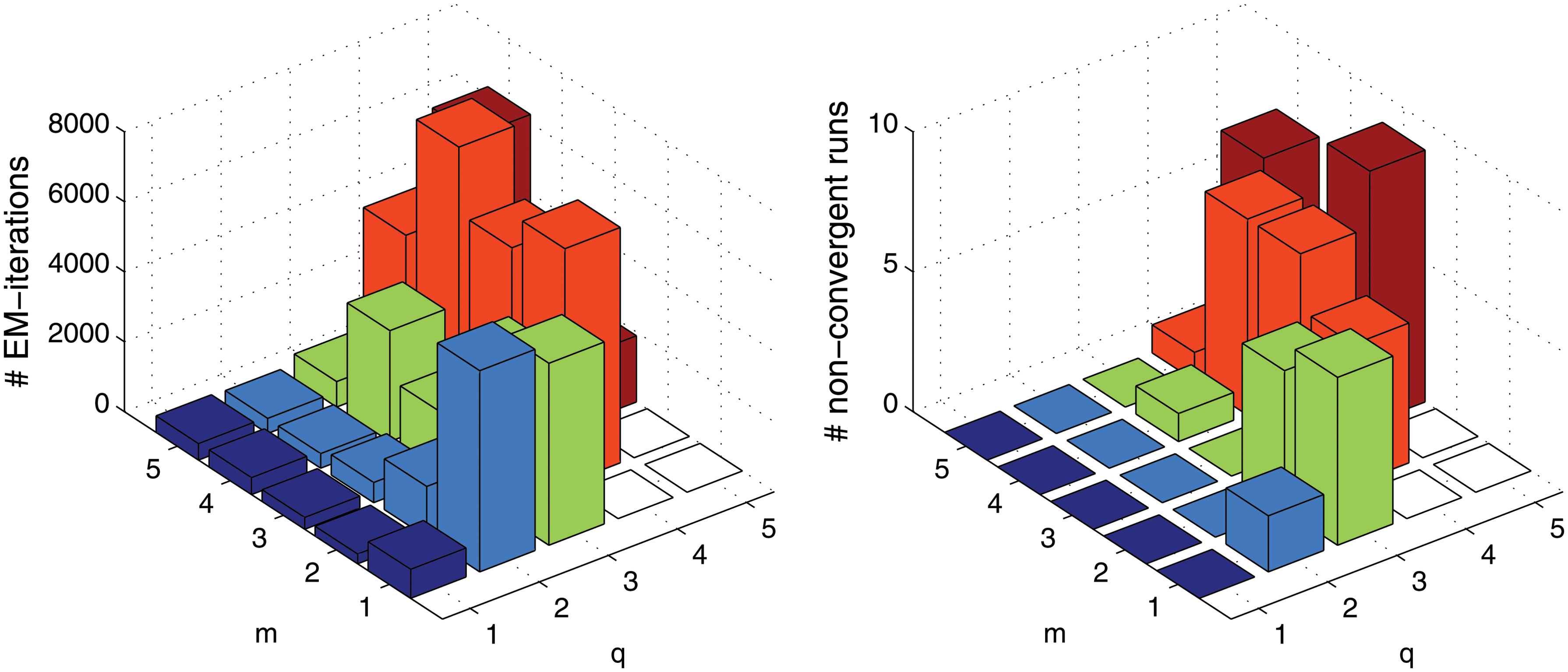end{document} (dimension of latent/observed variables). Figure 4 shows that for q<m the mean number of EM-steps is small, and for q>m or large dimensions q=m the number of EM-steps explodes and many runs do not converge at all. In blind source separation applications we usually assume q≤m, and we limit ourselves to such cases in the following.

OPEN IN VIEWER

FIG. 4.

Number of EM-iterations. We generate data from model (CC) and consider different combinations of \documentclass{aastex}\usepackage{amsbsy}\usepackage{amsfonts}\usepackage{amssymb}\usepackage{bm}\usepackage{mathrsfs}\usepackage{pifont}\usepackage{stmaryrd}\usepackage{textcomp}\usepackage{portland, xspace}\usepackage{amsmath, amsxtra}\pagestyle{empty}\DeclareMathSizes{10}{9}{7}{6}\begin{document} $$m , q = 1 , \ldots , 5$$ \end{document} (dimension of observed/latent variables). The plots show the mean number of EM-iterations among all convergent runs (left) and the number of nonconvergent runs (right). For all m/q-combinations with q≥m+2 we performed 10 runs of emGrade.

4.2. Algorithm comparison

We now compare emGrade to other blind source separation algorithms. The most similar algorithm regarding model assumptions is Grade, which diagonalizes the sample graph-delayed covariance using singular value decomposition. We distinguish between two versions—Grade(Pa) and Grade(E), where the graph-delayed covariance is estimated as \documentclass{aastex}\usepackage{amsbsy}\usepackage{amsfonts}\usepackage{amssymb}\usepackage{bm}\usepackage{mathrsfs}\usepackage{pifont}\usepackage{stmaryrd}\usepackage{textcomp}\usepackage{portland, xspace}\usepackage{amsmath, amsxtra}\pagestyle{empty}\DeclareMathSizes{10}{9}{7}{6}\begin{document} $$\hat{D}^{{\rm Pa}}$$ \end{document} and \documentclass{aastex}\usepackage{amsbsy}\usepackage{amsfonts}\usepackage{amssymb}\usepackage{bm}\usepackage{mathrsfs}\usepackage{pifont}\usepackage{stmaryrd}\usepackage{textcomp}\usepackage{portland, xspace}\usepackage{amsmath, amsxtra}\pagestyle{empty}\DeclareMathSizes{10}{9}{7}{6}\begin{document} $$\hat{D}^{\rm E}$$ \end{document} (section 2.1). We further consider algorithms for time-series data and simply resume the order of the random variables. AMUSE (Tong et al., 1990) and SOBI (Belouchrani et al., 1997) both assume stationarity (of the time-series), i.e. the autocovariance Cov ( x (i), x (i + τ)) is independent of the index i at any lag \documentclass{aastex}\usepackage{amsbsy}\usepackage{amsfonts}\usepackage{amssymb}\usepackage{bm}\usepackage{mathrsfs}\usepackage{pifont}\usepackage{stmaryrd}\usepackage{textcomp}\usepackage{portland, xspace}\usepackage{amsmath, amsxtra}\pagestyle{empty}\DeclareMathSizes{10}{9}{7}{6}\begin{document} $$\tau \in {\mathbb Z}$$ \end{document} . The algorithms then diagonalize sample autocovariances at one or multiple lags, respectively. Finally, we compare our results to PCA and fastICA (Hyvärinen and Oja, 2000), both act independently of the structure of the random variables.

All algorithms provide estimates of the mixing matrix and the source signals—but unlike emGrade they do not estimate the full parameter vector. θ=(A, μ, σ², D). Instead of a likelihood-based evaluation of the performance we use the distance of estimated and true mixing matrix as performance measure: \documentclass{aastex}\usepackage{amsbsy}\usepackage{amsfonts}\usepackage{amssymb}\usepackage{bm}\usepackage{mathrsfs}\usepackage{pifont}\usepackage{stmaryrd}\usepackage{textcomp}\usepackage{portland, xspace}\usepackage{amsmath, amsxtra}\pagestyle{empty}\DeclareMathSizes{10}{9}{7}{6}\begin{document} \begin{align*} { \rm dist } ( \hat { A } , A ) = \min_ { p \in { \cal P } } \frac { 1 } { \sqrt { mq } } \parallel \hat { A } P - A \parallel_F. \tag { 19 } \end{align*} \end{document}

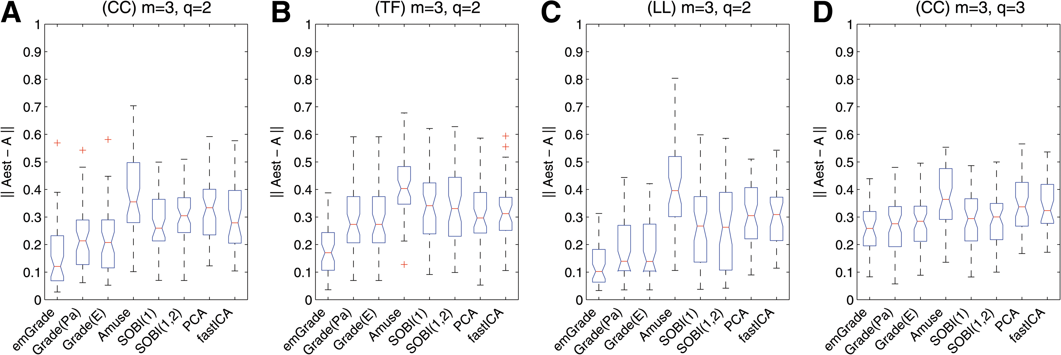
Let \documentclass{aastex}\usepackage{amsbsy}\usepackage{amsfonts}\usepackage{amssymb}\usepackage{bm}\usepackage{mathrsfs}\usepackage{pifont}\usepackage{stmaryrd}\usepackage{textcomp}\usepackage{portland, xspace}\usepackage{amsmath, amsxtra}\pagestyle{empty}\DeclareMathSizes{10}{9}{7}{6}\begin{document} $${ \cal P} \subseteq M \ at \, ( q , q )$$ \end{document} be the set of all q×q matrices with one nonzero entry per row and column and this entry has value ± 1. With this we correct for possible permutation and sign-changing of the mixing columns. If m-dimensional data is given all algorithms—except emGrade—estimate a mixing matrix in Mat(m,m). In case of q<m we only use the first q columns of the mixing estimates. In Figure 5 we compare the estimation performance of all algorithms, and we fix the dimensions at m=3 and q=2. For all proposed graph models emGrade outperforms the other algorithms in terms of correctness of the estimates, the drawback is a much higher run-time. In the case of m=q the improvement of the estimates is less apparent.

OPEN IN VIEWER

FIG. 5.

Algorithm comparison. The plots show the mean performance over 50 runs of the algorithms emGrade, Grade(G), Grade(E), AMUSE, SOBI (at lag 1 and at lags 1,2), PCA, and fastICA. In (A)–(C) we generated data from models (CC), (TF), and (LL) with m=3 and q=2. In this case (m>q) emGrade yields the best estimation performance for all graph models. In (C) where m=q=3 the improvement compared to the other algorithms is smaller.

4.3. Pathway identification and number of source signals

We now take full advantage of the probabilistic modeling and use model selection criteria to determine the correct number of source signals and to identify active pathways in the network. Let \documentclass{aastex}\usepackage{amsbsy}\usepackage{amsfonts}\usepackage{amssymb}\usepackage{bm}\usepackage{mathrsfs}\usepackage{pifont}\usepackage{stmaryrd}\usepackage{textcomp}\usepackage{portland, xspace}\usepackage{amsmath, amsxtra}\pagestyle{empty}\DeclareMathSizes{10}{9}{7}{6}\begin{document} $${ \cal M} ( G , q )$$ \end{document} denote the source model with q source signals, and the joint distribution is based on a weighted graph G. We then consider the following information criterion: \documentclass{aastex}\usepackage{amsbsy}\usepackage{amsfonts}\usepackage{amssymb}\usepackage{bm}\usepackage{mathrsfs}\usepackage{pifont}\usepackage{stmaryrd}\usepackage{textcomp}\usepackage{portland, xspace}\usepackage{amsmath, amsxtra}\pagestyle{empty}\DeclareMathSizes{10}{9}{7}{6}\begin{document} \begin{align*}{ \rm IC} ( { \cal M} ( G , q ) ) = - 2 \ell ( \theta;X , { \cal M} ( G , q ) ) + kc , \tag{20}\end{align*} \end{document}

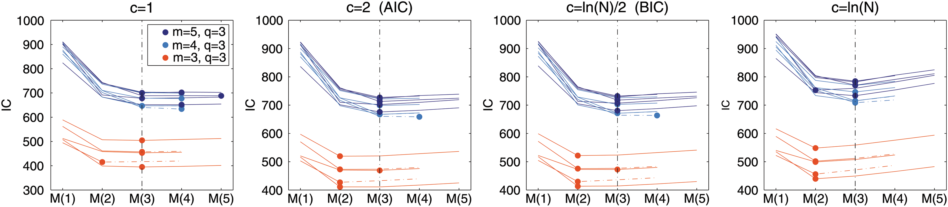
where k denotes the number of model parameters, and c is some constant. For c=2 the above equation yields the Akaike information criterion (AIC) (Akaike, 1974) and for c=ln(N) the equation yields the Bayesian information criterion (BIC) (Schwarz, 1978) with N the number of observed variables. To determine the true number of source signals we fix the graph G and search for the lowest IC value among different source models. Since the comparison is based on the log-likelihood value of the emGrade estimates we use \documentclass{aastex}\usepackage{amsbsy}\usepackage{amsfonts}\usepackage{amssymb}\usepackage{bm}\usepackage{mathrsfs}\usepackage{pifont}\usepackage{stmaryrd}\usepackage{textcomp}\usepackage{portland, xspace}\usepackage{amsmath, amsxtra}\pagestyle{empty}\DeclareMathSizes{10}{9}{7}{6}\begin{document} $$\mid \ell ( \theta; \ \textbf{\textit{X}} ) - \ell ( \theta^{ ( new ) }; \ \textbf{\textit{X}} ) \mid < $$ \end{document} 10⁻⁶ as convergence criterion. In Figure 6 we generated data from model (CC) with q=3 the true number of source signals (dimension of the latent variables) and m=3, 4, 5 observations (dimension of the observed variables). We then compare the IC values of \documentclass{aastex}\usepackage{amsbsy}\usepackage{amsfonts}\usepackage{amssymb}\usepackage{bm}\usepackage{mathrsfs}\usepackage{pifont}\usepackage{stmaryrd}\usepackage{textcomp}\usepackage{portland, xspace}\usepackage{amsmath, amsxtra}\pagestyle{empty}\DeclareMathSizes{10}{9}{7}{6}\begin{document} $$M ( \hat{q} ) = { \cal M} ( ( CC ) , \hat{q} )$$ \end{document} for \documentclass{aastex}\usepackage{amsbsy}\usepackage{amsfonts}\usepackage{amssymb}\usepackage{bm}\usepackage{mathrsfs}\usepackage{pifont}\usepackage{stmaryrd}\usepackage{textcomp}\usepackage{portland, xspace}\usepackage{amsmath, amsxtra}\pagestyle{empty}\DeclareMathSizes{10}{9}{7}{6}\begin{document} $$\hat{q} = 1 , \ldots , 5$$ \end{document} , where we consider different constant values c. In case of m > q we find a nearly perfect estimation of the true number of source signals for c=2 (AIC) and c=ln(N) (BIC).

OPEN IN VIEWER

FIG. 6.

Estimation of the number of source signals. We generate data from model (CC) with q=3 source signals (dimension of the latent variables) and m-dimensional observations for m=5,4,3 in different colors. For the graph-delayed covariance we consider D=[0.7,−0.49,0.3]. The plots show the IC values of all source models \documentclass{aastex}\usepackage{amsbsy}\usepackage{amsfonts}\usepackage{amssymb}\usepackage{bm}\usepackage{mathrsfs}\usepackage{pifont}\usepackage{stmaryrd}\usepackage{textcomp}\usepackage{portland, xspace}\usepackage{amsmath, amsxtra}\pagestyle{empty}\DeclareMathSizes{10}{9}{7}{6}\begin{document} $$M ( \hat{q} ) = { \cal M} ( ( { \rm CC} ) , \hat{q} )$$ \end{document} for increasing \documentclass{aastex}\usepackage{amsbsy}\usepackage{amsfonts}\usepackage{amssymb}\usepackage{bm}\usepackage{mathrsfs}\usepackage{pifont}\usepackage{stmaryrd}\usepackage{textcomp}\usepackage{portland, xspace}\usepackage{amsmath, amsxtra}\pagestyle{empty}\DeclareMathSizes{10}{9}{7}{6}\begin{document} $$\hat{q} = 1 , \ldots , 5$$ \end{document} . In each plot we consider a different constant c. The black vertical lines show the true number of source signals and the dots indicate the selected source model in each comparison, that is, the model with the lowest IC value. Dashed lines lead to IC values of nonconvergent runs (using the log-likelihood value after 10,000 iterations), and some IC values are +∞. IC, information criterion.

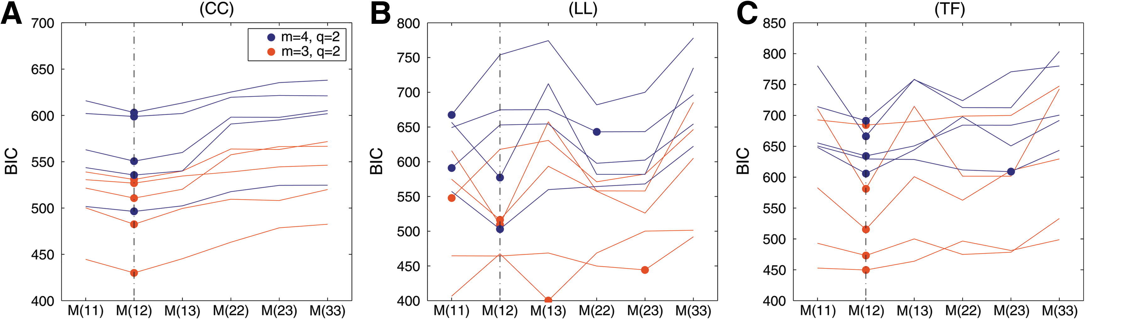
For pathway identification we divide each network from section 2.2 into three pathways (subnetworks) P₁, P₂, and P₃. For (CC) we define the pathways as the three connected components of the complete cell-cycle network, for (TF) we consider the single hub-nodes together with their target nodes as pathways, and for (LL) we consider the two overlapping lines and the additional line as pathways. We then generate data from the pathway source model \documentclass{aastex}\usepackage{amsbsy}\usepackage{amsfonts}\usepackage{amssymb}\usepackage{bm}\usepackage{mathrsfs}\usepackage{pifont}\usepackage{stmaryrd}\usepackage{textcomp}\usepackage{portland, xspace}\usepackage{amsmath, amsxtra}\pagestyle{empty}\DeclareMathSizes{10}{9}{7}{6}\begin{document} $${ \cal M} ( P_i , P_j )$$ \end{document} introduced in section 3.4, and we determine the lowest IC value among all source models \documentclass{aastex}\usepackage{amsbsy}\usepackage{amsfonts}\usepackage{amssymb}\usepackage{bm}\usepackage{mathrsfs}\usepackage{pifont}\usepackage{stmaryrd}\usepackage{textcomp}\usepackage{portland, xspace}\usepackage{amsmath, amsxtra}\pagestyle{empty}\DeclareMathSizes{10}{9}{7}{6}\begin{document} $$M ( i , j ) = { \cal M} ( P_i , P_j )$$ \end{document} for i,j=1,2,3. If the edges of the pathways are nonoverlapping [models (CC) and (TF)] we observe a good pathway identification; for model (LL) often only one pathway is identified correctly (Fig. 7).

OPEN IN VIEWER

FIG. 7.

Pathway identification. We generate q=2 source signals from the respective pathways P₁ and P₂ of the models (CC), (LL), and (TF). From observations of dimension m=4,3 (in different colors) we calculate the BIC of all pathway source models \documentclass{aastex}\usepackage{amsbsy}\usepackage{amsfonts}\usepackage{amssymb}\usepackage{bm}\usepackage{mathrsfs}\usepackage{pifont}\usepackage{stmaryrd}\usepackage{textcomp}\usepackage{portland, xspace}\usepackage{amsmath, amsxtra}\pagestyle{empty}\DeclareMathSizes{10}{9}{7}{6}\begin{document} $$M ( i , j ) = { \cal M} ( P_i , P_j )$$ \end{document} , where we assume source signals from pathways P_i and P_j (i,j=1,2,3). The black vertical lines show the true pathway combination, and the dots indicate the selected source model in each comparison, that is, the model with the lowest BIC value. BIC, Bayesian information criterion.