The Worst Case Complexity of Maximum Parsimony

1. Introduction

Phylogenetics is the study of evolutionary relationships among groups of organisms (e.g., species, populations), which are discovered through molecular sequencing data and morphological data matrices. A phylogeny (also called a dendogram) is a graphlike structure whose topology describes the inferred evolutionary history among a set of biological entities, such as species or DNA sequences.

Phylogenies are classically modeled as either rooted or unrooted labeled binary trees, where the input entities are assigned to the leaf vertices. An unrooted phylogeny is an acyclic connected labeled graph in which every vertex has a degree of either three or one. Each vertex of degree one has a distinct label. A rooted phylogeny, on the other hand, is similar to an unrooted phylogeny, except that it has one internal vertex of degree two, which is designated as the root. In a rooted phylogeny the edges are directed from the root toward the leaves.

The decision of whether to model phylogenies as rooted versus unrooted trees depends either on the availability of a molecular clock, or on the nucleotide or amino acid substitution scoring matrix representing the evolutionary mutation events. Modeling phylogenies as unrooted trees requires the assumption of symmetric scoring matrices. However, when the symmetry restriction on scoring matrices is removed, the tree rooting becomes meaningful. A simple literature review of current biological research shows that the symmetric scoring matrices, though computationally convenient, do not yield a biologically reliable model (Rodriguez et al., 1990; Takahata and Kimura, 1981; Gojobori et al., 1982; Tajima and Nei, 1984). Various recent biological publications apply asymmetric scoring matrices to the alignment of genomic sequences, and many articles can nowadays be found on the construction of asymmetric scoring matrices consisting of nucleotides (Tamura, 1992; Tamura and Nei, 1993; Blouin et al., 1998) and amino acids (Müller et al., 2001; Bastien et al., 2005). Thus, in this work we do not assume symmetric scoring matrices and therefore construct rooted phylogenies.

Methods for phylogeny reconstruction can be classified into distance-based versus character-based methods. Given a set of input sequences, a distance-based method, such as UPGMA and neighbor joining (NJ), first computes pairwise distances according to some measure (Felsenstein and Felenstein, 2004). Then, the actual data is discarded and the fixed distances are used in the derivation of trees. In contrast, in character-based methods (such as maximum parsimony and maximum likelihood) the inference depends upon models describing the evolutionary changes of characters (e.g., nucleotides or amino acids) that led from an original sequence in some common ancestor to the evolution of the observed input sequences. The great advantage of character-based algorithms for phylogenetic reconstruction is that, given a good multiple alignment of input sequences, they can exploit the potential phylogenetic inferences with great sensitivity. Their weakness, however, is in their computational intensity. In this article we focus on the classical maximum parsimony character-based phylogenetic approach.

1.1. Phylogentic reconstruction based on parsimony maximization

Parsimony maximization (i.e., preferring the simpler of two otherwise equally adequate theorizations) is one of the classical approaches to computationally reconstruct a phylogeny for a given set of biologically related sequences. When applied to computational phylogenetics, the parsimony maximization approach seeks the phylogenetic tree that supposes the least amount of evolutionary change explaining the observed data (Cavalli-Sforza and Edwards, 1967). There are two classical problems inferred from phylogenetic parsimony maximization: small parsimony (SP) and maximum parsimony (MP), as explained below.

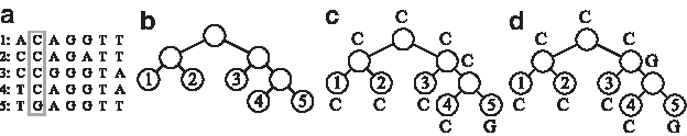
Problem 1: Small parsimony (SP) The small parsimony problem is to compute, for a proposed phylogeny, a reconstruction of events leading to the input data with as few changes as possible over the whole tree (Fig. 1). The input to this problem is a multiple alignment of n input sequences of length m each, and a topology in the form of a rooted phylogenetic tree over n leaves, where each leaf is associated with a distinct sequence from the input set. Based on this input, the objective is to compute a labeling of the internal vertices of the input phylogeny that optimizes some predefined scoring scheme.

OPEN IN VIEWER

FIG. 1.

An example of an instance with Hamming distance–based parsimony score. The input to the problem consists of five species and a multiple alignment of their corresponding sequences (a) and a given phylogeny (b). Note that the phylogeny specification consists of both the tree topology and the assignments of species to its leaves. In this example, n = 5 and m = 7; (c) and (d) show two examples of internal vertices assignments corresponding to the second state (column) of the exemplified SP instance [highlighted in (a) via a gray rectangle]. A binary substitution scoring matrix is assumed in this scoring scheme, where two identical characters are given a score of 0, and two distinct characters a score of 1. Assignment (c) provides the minimal number of mutations, 1, whereas assignment (d) yields two character mutations.

The most basic algorithms for solving SP are Fitch's algorithm (Fitch, 1971) and Sankoff's algorithm (Sankoff, 1975). In its simplest variant (solved by Fitch's algorithm and exemplified in Fig. 1c and d), the scoring scheme is Hamming distance, and the optimal labeling is one that minimizes the number of mutations. It is standard to assume position-independence between the states (columns of characters in the multiple alignment). Thus, the total SP score for an input multiple sequence alignment is computed as the sum of the SP scores of each state assignment.

Problem 2: Maximum parsimony (MP) The maximum parsimony (MP) problem is to seek, among all possible phylogenies over a given set of leaves, the phylogeny that yields the best SP score. Similarly to SP, the input to this problem is a multiple alignment of n input sequences of length m each. However, here the topology is not given. The MP problem is NP-hard (Day and Sankoff, 1986; Foulds and Graham, 1982). A straightforward approach for solving MP is to enumerate all possible phylogenies over the set of leaves and then employ an SP algorithm on each phylogeny. This approach was used by Cavalli-Sforza and Edwards (1967), who showed that the number of phylogenies over n leaves is \documentclass{aastex}\usepackage{amsbsy}\usepackage{amsfonts}\usepackage{amssymb}\usepackage{bm}\usepackage{mathrsfs}\usepackage{pifont}\usepackage{stmaryrd}\usepackage{textcomp}\usepackage{portland, xspace}\usepackage{amsmath, amsxtra}\pagestyle{empty}\DeclareMathSizes{10}{9}{7}{6}\begin{document} $$( 2n - 3 ) !! = 1 \times 3 \times 5 \times \cdots \times ( 2n - 3 )$$ \end{document} . Several constrained variants of MP were studied over the years (Felsenstein and Felenstein, 2004). The most famous among them is the perfect phylogeny problem, which is also NP-hard (Bodlaender et al., 1992) and for which FPT algorithms were proposed (Agarwala and Fernández-Baca, 1994; McMorris et al., 1993).

Measuring SP and MP complexity in terms of basic operations. SP and MP algorithms work by computing some information for every internal vertex of the input phylogeny. This information, as well as the complexity of its computation, depend on the scoring scheme employed by the parsimony algorithm. Thus, in what follows, we will use the term basic operation to denote the work invested in the computation of the information of a single vertex of a considered phylogeny for a specific scoring scheme. For example, in the Fitch SP algorithm (Fitch, 1971), which computes a minimal Hamming distance SP score, an O(m)-time basic operation is applied, while in the Sankoff algorithm (Sankoff, 1975), which optimizes an SP score of minimal weighted edit distance, an O(mΣ²)-time basic operation is applied, where Σ denotes the size of the alphabet spelling the input sequences.

Our Contribution In this work, we examine the complexity of MP in terms of the total number of basic operations executed throughout the run of the algorithm. Using this measure, we analyze the worst case complexity of three approaches to MP. The first, basic approach, is the one proposed by Cavalli-Sforza and Edwards (1967), which performs (n−1) · (2n−3)!! basic operations. The second approach is based on the Hendy and Penny (1982) MP search space, which interleaves the SP computations within the tree-space development flow. This search space was originally proposed for the purpose of a branch-and-bound MP search, and its theoretical worst-case bound was not previously properly bounded. Our first result is Theorem 2.2 in section 2, in which we analyze the basic operations complexity of the Hendy and Penny approach and show that it is faster than the Cavalli-Sforza and Edwards approach by a factor of \documentclass{aastex}\usepackage{amsbsy}\usepackage{amsfonts}\usepackage{amssymb}\usepackage{bm}\usepackage{mathrsfs}\usepackage{pifont}\usepackage{stmaryrd}\usepackage{textcomp}\usepackage{portland, xspace}\usepackage{amsmath, amsxtra}\pagestyle{empty}\DeclareMathSizes{10}{9}{7}{6}\begin{document} $$\Theta ( \sqrt{n} )$$ \end{document} .

Both Hendy and Penny's work as well as the follow-up exact branch and bound extensions (Felsenstein and Felenstein, 2004) still kept the same traditional order of search space development, based on the Cavalli-Sforza and Edwards tree enumeration order. In order to further improve MP efficiency, we propose to turn the state development order of the classical MP search tree “upside down,” that is, from the classical top down incremental tree extension by a single edge per each new state, to a bottom-up agglomerative approach that merges two previous subtrees per each state. This idea is based on the observation that the “top down” approach to MP search goes “against the grain” of the update operations applied by the Hendy and Penny SP subroutines per each new search space node.

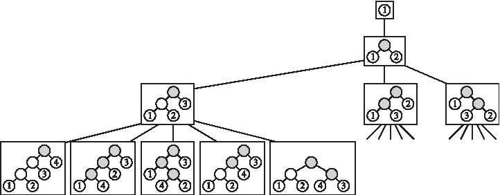
Due to this, the savings by the Hendy and Penny approach in avoiding overlapping redundant SP computations across subtrees shared by distinct phylogenies at level n is weakened by the work applied for the sake of search-space information maintenance. Such maintenance requires, per each new node in the search space, the traversal and updates of all vertices along the path from the newly added leaf up to the root of the phylogeny represented by the new node (Fig. 2).

OPEN IN VIEWER

FIG. 2.

An example of the search space tree \documentclass{aastex}\usepackage{amsbsy}\usepackage{amsfonts}\usepackage{amssymb}\usepackage{bm}\usepackage{mathrsfs}\usepackage{pifont}\usepackage{stmaryrd}\usepackage{textcomp}\usepackage{portland, xspace}\usepackage{amsmath, amsxtra}\pagestyle{empty}\DeclareMathSizes{10}{9}{7}{6}\begin{document} $${ \cal T}_4^{{ \rm CSE}}$$ \end{document} . Only some of the nodes of the search space tree are shown. Highlighted in gray within the phylogenies in each node of the search tree are the vertices updated by basic operations when applying Hendy and Penny's MP approach on \documentclass{aastex}\usepackage{amsbsy}\usepackage{amsfonts}\usepackage{amssymb}\usepackage{bm}\usepackage{mathrsfs}\usepackage{pifont}\usepackage{stmaryrd}\usepackage{textcomp}\usepackage{portland, xspace}\usepackage{amsmath, amsxtra}\pagestyle{empty}\DeclareMathSizes{10}{9}{7}{6}\begin{document} $${ \cal T}_4^{{ \rm CSE}}$$ \end{document} .

In order to avoid this inefficiency, we suggest a “bottom up” directed MP search, based on subtree merging, which flows along with the natural “bottom up” direction of small parsimony. By design, traversing the search space according to our proposed search tree requires performing exactly one basic operation per node of the search tree (the basic operation is applied on the new root of the two merged trees in the agglomerative step). Thus, the complexity of our new MP algorithm is equal to the size of our proposed search space tree. We show that this size is approximately e · (2n – 3)!!, where e is the base of the natural logarithm. Thus, our new approach yields a basic operations complexity that is smaller by a factor of \documentclass{aastex}\usepackage{amsbsy}\usepackage{amsfonts}\usepackage{amssymb}\usepackage{bm}\usepackage{mathrsfs}\usepackage{pifont}\usepackage{stmaryrd}\usepackage{textcomp}\usepackage{portland, xspace}\usepackage{amsmath, amsxtra}\pagestyle{empty}\DeclareMathSizes{10}{9}{7}{6}\begin{document} $$\Theta ( \sqrt{n} )$$ \end{document} than the complexity of the Hendy and Penny approach (Theorem 3 in section 4). We note that the bound obtained by our proposed algorithm is on the same order of the number of topologies considered by MP, and therefore any approach to exact MP that must enumerate all topologies will not improve our result.

We note that the original work of Hendy and Penny assumed a symmetric scoring matrix. Under the assumption of symmetric scoring matrices, it can be shown that rooted MP can be solved via the simpler unrooted MP. However, such is not the case in practice, when the restriction to symmetrical scoring matrices is removed (Rodriguez et al., 1990; Takahata and Kimura, 1981; Gojobori et al., 1982; Tajima and Nei, 1984), and the tree rooting becomes meaningful. The algorithms we propose and analyze in this article generalize the previous most efficient exact solutions to this problem and do not assume the use of symmetrical scoring matrices.

The rest of the article proceeds as follows. First, in section 2 we analyze the basic operations complexity of the algorithm of Cavalli-Sforza and Edwards and the algorithm of Hendy and Penny. In section 3 we describe our new approach to search space construction, and in section 4 we analyze the basic operations complexity of our search space. Finally, we give our concluding remarks in section 5.

2. Analysis of Previous Approaches

Throughout the article, a phylogeny is a rooted binary labeled tree. Each leaf in the tree has a distinct label from \documentclass{aastex}\usepackage{amsbsy}\usepackage{amsfonts}\usepackage{amssymb}\usepackage{bm}\usepackage{mathrsfs}\usepackage{pifont}\usepackage{stmaryrd}\usepackage{textcomp}\usepackage{portland, xspace}\usepackage{amsmath, amsxtra}\pagestyle{empty}\DeclareMathSizes{10}{9}{7}{6}\begin{document} $$\{ 1 , \ldots , n \} $$ \end{document} , where n is the number of leaves. We also define a forest to be a collection of rooted binary labeled trees. Each leaf in the forest has a distinct label from \documentclass{aastex}\usepackage{amsbsy}\usepackage{amsfonts}\usepackage{amssymb}\usepackage{bm}\usepackage{mathrsfs}\usepackage{pifont}\usepackage{stmaryrd}\usepackage{textcomp}\usepackage{portland, xspace}\usepackage{amsmath, amsxtra}\pagestyle{empty}\DeclareMathSizes{10}{9}{7}{6}\begin{document} $$\{ 1 , \ldots , n \} $$ \end{document} , where n is the number of leaves in all the trees.

We will later define another type of trees called search space trees. In order to make the text more clear, we will use different terminology for the two types of trees; we will use vertex for phylogenies and node for search space trees.

2.2. The algorithm of Hendy and Penny

Hendy and Penny (1982) interleaved the small parsimony operations within search space tree traversal. Their algorithm traverses the tree \documentclass{aastex}\usepackage{amsbsy}\usepackage{amsfonts}\usepackage{amssymb}\usepackage{bm}\usepackage{mathrsfs}\usepackage{pifont}\usepackage{stmaryrd}\usepackage{textcomp}\usepackage{portland, xspace}\usepackage{amsmath, amsxtra}\pagestyle{empty}\DeclareMathSizes{10}{9}{7}{6}\begin{document} $${ \cal T}_n^{{ \rm CSE}}$$ \end{document} , and when reaching a node v, it solves the small parsimony problem for the phylogeny F_v. However, the small parsimony algorithm does not need to compute the required information for all internal vertices of F_v since the information computed for the phylogeny of v's parent can be used. More precisely, let u be the parent of v, and let x be the newly added leaf in F_v. If y is an internal vertex of F_v that is not an ancestor of x, then the information for the vertex y in F_v is identical to the information for the vertex y in F_u. Since the latter was already computed, in order to solve the small parsimony problem on F_v, only vertex information for the ancestors of x needs to be computed. For a vertex v in \documentclass{aastex}\usepackage{amsbsy}\usepackage{amsfonts}\usepackage{amssymb}\usepackage{bm}\usepackage{mathrsfs}\usepackage{pifont}\usepackage{stmaryrd}\usepackage{textcomp}\usepackage{portland, xspace}\usepackage{amsmath, amsxtra}\pagestyle{empty}\DeclareMathSizes{10}{9}{7}{6}\begin{document} $${ \cal T}_n^{{ \rm CSE}}$$ \end{document} , let NumAnc(v) denote the number of ancestors of x in F_v, where x is the newly added leaf in F_v. Therefore, the basic operations complexity of the algorithm of Hendy and Penny is \documentclass{aastex}\usepackage{amsbsy}\usepackage{amsfonts}\usepackage{amssymb}\usepackage{bm}\usepackage{mathrsfs}\usepackage{pifont}\usepackage{stmaryrd}\usepackage{textcomp}\usepackage{portland, xspace}\usepackage{amsmath, amsxtra}\pagestyle{empty}\DeclareMathSizes{10}{9}{7}{6}\begin{document} $$\sum\nolimits_{v \in { \cal T}_n^{{ \rm CSE}}}$$ \end{document} NumAnc(v) (the summation is performed over nodes from all levels of the search tree). We next give a formula for the summation above.

Definition 1. Let H_i be the sum of NumAnc(v) for all nodes v in level i+1 of \documentclass{aastex}\usepackage{amsbsy}\usepackage{amsfonts}\usepackage{amssymb}\usepackage{bm}\usepackage{mathrsfs}\usepackage{pifont}\usepackage{stmaryrd}\usepackage{textcomp}\usepackage{portland, xspace}\usepackage{amsmath, amsxtra}\pagestyle{empty}\DeclareMathSizes{10}{9}{7}{6}\begin{document} $${ \cal T}_n^{{ \rm CSE}}$$ \end{document} .

By definition, \documentclass{aastex}\usepackage{amsbsy}\usepackage{amsfonts}\usepackage{amssymb}\usepackage{bm}\usepackage{mathrsfs}\usepackage{pifont}\usepackage{stmaryrd}\usepackage{textcomp}\usepackage{portland, xspace}\usepackage{amsmath, amsxtra}\pagestyle{empty}\DeclareMathSizes{10}{9}{7}{6}\begin{document} $$\sum \nolimits_{v \in { \cal T}_n^{{ \rm CSE}}}{ \rm NumAnc} ( v ) = \sum \nolimits_{i = 1}^{n - 1} H_i$$ \end{document} .

Lemma 1. H_i=(2i)!!−(2i−1)!!.

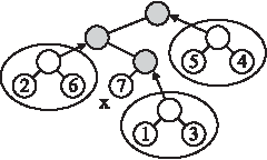
Proof. Let v be a node at level i+1 in \documentclass{aastex}\usepackage{amsbsy}\usepackage{amsfonts}\usepackage{amssymb}\usepackage{bm}\usepackage{mathrsfs}\usepackage{pifont}\usepackage{stmaryrd}\usepackage{textcomp}\usepackage{portland, xspace}\usepackage{amsmath, amsxtra}\pagestyle{empty}\DeclareMathSizes{10}{9}{7}{6}\begin{document} $${ \cal T}_n^{{ \rm CSE}}$$ \end{document} , and let x be the newly added leaf in F_v. Let F′ be the forest obtained from F_v by removing x and its ancestors, and removing all the edges incident on these vertices. Note that every tree in F′ is a subtree of a distinct ancestor of x in F_v, and every ancestor of x corresponds to exactly one tree in F′. Therefore, NumAnc(v) is equal to the number of trees in F′ (see Fig. 3 for an example). The latter number is called the cover number for \documentclass{aastex}\usepackage{amsbsy}\usepackage{amsfonts}\usepackage{amssymb}\usepackage{bm}\usepackage{mathrsfs}\usepackage{pifont}\usepackage{stmaryrd}\usepackage{textcomp}\usepackage{portland, xspace}\usepackage{amsmath, amsxtra}\pagestyle{empty}\DeclareMathSizes{10}{9}{7}{6}\begin{document} $$\{ 1 , \ldots , i \} $$ \end{document} in F_v in Ochiumi et al. (2011). It is shown in Ochiumi et al. (2011) that the sum of the cover number for \documentclass{aastex}\usepackage{amsbsy}\usepackage{amsfonts}\usepackage{amssymb}\usepackage{bm}\usepackage{mathrsfs}\usepackage{pifont}\usepackage{stmaryrd}\usepackage{textcomp}\usepackage{portland, xspace}\usepackage{amsmath, amsxtra}\pagestyle{empty}\DeclareMathSizes{10}{9}{7}{6}\begin{document} $$\{ 1 , \ldots , i \} $$ \end{document} in all phylogenies with i+1 leaves is (2i)!!−(2i−1)!!.   ■

OPEN IN VIEWER

FIG. 3.

An example for the proof of Lemma 1. The leaf x has three ancestors, which is equal to the number of trees in the forest obtained by removing x and its ancestors.

Theorem 2. The basic operations complexity of the algorithm of Hendy and Penny is \documentclass{aastex}\usepackage{amsbsy}\usepackage{amsfonts}\usepackage{amssymb}\usepackage{bm}\usepackage{mathrsfs}\usepackage{pifont}\usepackage{stmaryrd}\usepackage{textcomp}\usepackage{portland, xspace}\usepackage{amsmath, amsxtra}\pagestyle{empty}\DeclareMathSizes{10}{9}{7}{6}\begin{document} $$\Theta ( \sqrt{n} ( 2n - 3 ) !! )$$ \end{document} .

Proof. By Lemma 1, the complexity is \documentclass{aastex}\usepackage{amsbsy}\usepackage{amsfonts}\usepackage{amssymb}\usepackage{bm}\usepackage{mathrsfs}\usepackage{pifont}\usepackage{stmaryrd}\usepackage{textcomp}\usepackage{portland, xspace}\usepackage{amsmath, amsxtra}\pagestyle{empty}\DeclareMathSizes{10}{9}{7}{6}\begin{document} $$\sum \nolimits_{i = 1}^{n - 1} ( ( 2i ) !! - ( 2i - 1 ) !! )$$ \end{document} . We have \documentclass{aastex}\usepackage{amsbsy}\usepackage{amsfonts}\usepackage{amssymb}\usepackage{bm}\usepackage{mathrsfs}\usepackage{pifont}\usepackage{stmaryrd}\usepackage{textcomp}\usepackage{portland, xspace}\usepackage{amsmath, amsxtra}\pagestyle{empty}\DeclareMathSizes{10}{9}{7}{6}\begin{document} \begin{align*} \lim_{n \rightarrow \infty} & \frac {\sum_{i = 1}^{n - 1} ((2i) !! - (2i - 1) !!)} {\sqrt {n} (2n - 3) !!} \\ = & \lim_ { n \rightarrow \infty } \left( \frac {\sum\limits_{i = 1}^{n - 2} ((2i ) !! - ( 2i - 1 ) !! ) } { \sqrt { n } ( 2n - 3 ) !! } + \frac { ( 2n - 2 ) !! - ( 2n - 3 ) !! } { \sqrt { n } ( 2n - 3 ) !! } \right) \\ & \mathop=^ { ( 1 ) } \lim_ { n \rightarrow \infty } \frac { ( 2n - 2 ) !! - ( 2n - 3 ) !! } { \sqrt { n } ( 2n - 3 ) !! } = \lim_ { n \rightarrow \infty } \frac { ( 2n - 2 ) !! } { \sqrt { n } ( 2n - 3 ) !! } \\ & \qquad = \lim_ { n \rightarrow \infty } \frac {(2n) !!} {\sqrt {n} (2n - 1) !!} \mathop=^{(2)} \lim_ { n \rightarrow \infty } \frac { ( 2n ) ! } { \sqrt { n } ( ( 2n - 1 ) !! ) ^2 } \\ & \mathop=^ { ( 3 ) } \lim_ { n \rightarrow \infty } \frac { ( 2n ) ! } { \sqrt { n } \left( \frac { ( 2n ) ! } { 2^ { n } \cdot n! } \right) ^2 } = \lim_ { n \rightarrow \infty } \frac { ( 2^nn! ) ^2 } { \sqrt { n } ( 2n ) ! } \mathop=^ { ( 4 ) } \lim_ { n \rightarrow \infty } \frac { 2 \pi n ( \frac { 2n } { e } ) ^ { 2n } } {\sqrt{n} \sqrt {4 \pi n} (\frac {2n} {e})^{2n}} = \sqrt {\pi} . \end{align*} \end{document}

Equality (1) is true since \documentclass{aastex}\usepackage{amsbsy}\usepackage{amsfonts}\usepackage{amssymb}\usepackage{bm}\usepackage{mathrsfs}\usepackage{pifont}\usepackage{stmaryrd}\usepackage{textcomp}\usepackage{portland, xspace}\usepackage{amsmath, amsxtra}\pagestyle{empty}\DeclareMathSizes{10}{9}{7}{6}\begin{document} \begin{align*}\sum\limits_{i = 1}^{n - 2} ( ( 2i ) !! - ( 2i - 1 ) !! ) = ( 2n - 4 ) !! - 1!! + \left( \sum\limits_{i = 2}^{n - 2} ( 2i - 2 ) !! - ( 2i - 1 ) !! \right) \leq ( 2n - 4 ) !!.\end{align*} \end{document}

Therefore, the limit of the summation above divided by \documentclass{aastex}\usepackage{amsbsy}\usepackage{amsfonts}\usepackage{amssymb}\usepackage{bm}\usepackage{mathrsfs}\usepackage{pifont}\usepackage{stmaryrd}\usepackage{textcomp}\usepackage{portland, xspace}\usepackage{amsmath, amsxtra}\pagestyle{empty}\DeclareMathSizes{10}{9}{7}{6}\begin{document} $$\sqrt{n} ( 2n - 3 ) !!$$ \end{document} is 0. Equality (2) follows from the equality (2n)!=(2n)!!(2n−1)!!. Equality (3) follows from the equalities (2n)!!=2 ⁿ ·n! and (2n)!=(2n)!!(2n−1)!!. Finally, Equality (4) follows from Stirling's formula.   ■

3. A New, More Efficient Search Space Tree

In this section we present a new, “bottom up” search space enumerating MP. In order to define our new search space tree, we first build a directed acyclic graph \documentclass{aastex}\usepackage{amsbsy}\usepackage{amsfonts}\usepackage{amssymb}\usepackage{bm}\usepackage{mathrsfs}\usepackage{pifont}\usepackage{stmaryrd}\usepackage{textcomp}\usepackage{portland, xspace}\usepackage{amsmath, amsxtra}\pagestyle{empty}\DeclareMathSizes{10}{9}{7}{6}\begin{document} $${ \cal G}_n$$ \end{document} . We will later transform \documentclass{aastex}\usepackage{amsbsy}\usepackage{amsfonts}\usepackage{amssymb}\usepackage{bm}\usepackage{mathrsfs}\usepackage{pifont}\usepackage{stmaryrd}\usepackage{textcomp}\usepackage{portland, xspace}\usepackage{amsmath, amsxtra}\pagestyle{empty}\DeclareMathSizes{10}{9}{7}{6}\begin{document} $${ \cal G}_n$$ \end{document} into a tree \documentclass{aastex}\usepackage{amsbsy}\usepackage{amsfonts}\usepackage{amssymb}\usepackage{bm}\usepackage{mathrsfs}\usepackage{pifont}\usepackage{stmaryrd}\usepackage{textcomp}\usepackage{portland, xspace}\usepackage{amsmath, amsxtra}\pagestyle{empty}\DeclareMathSizes{10}{9}{7}{6}\begin{document} $${ \cal T}_n$$ \end{document} by removing some of the edges.

We define a merge operation on a forest F to be an operation that generates a new forest F′ by adding a new vertex to the forest and hanging two trees of F on this vertex. In the graph \documentclass{aastex}\usepackage{amsbsy}\usepackage{amsfonts}\usepackage{amssymb}\usepackage{bm}\usepackage{mathrsfs}\usepackage{pifont}\usepackage{stmaryrd}\usepackage{textcomp}\usepackage{portland, xspace}\usepackage{amsmath, amsxtra}\pagestyle{empty}\DeclareMathSizes{10}{9}{7}{6}\begin{document} $${ \cal G}_n$$ \end{document} , every node v corresponds to a forest with n leaves. The graph contains a single node at level 0 whose corresponding forest consists of n singletons. The nodes of level i in the graph correspond to all the forests that can be obtained from the forests that correspond to the nodes of level i−1 by single merge operations. There is an edge (u, v) in the graph if and only if F_v is obtained from F_u by a merge operation.

Note that a node in \documentclass{aastex}\usepackage{amsbsy}\usepackage{amsfonts}\usepackage{amssymb}\usepackage{bm}\usepackage{mathrsfs}\usepackage{pifont}\usepackage{stmaryrd}\usepackage{textcomp}\usepackage{portland, xspace}\usepackage{amsmath, amsxtra}\pagestyle{empty}\DeclareMathSizes{10}{9}{7}{6}\begin{document} $${ \cal G}_n$$ \end{document} can have several incoming edges. We next transform n into a tree \documentclass{aastex}\usepackage{amsbsy}\usepackage{amsfonts}\usepackage{amssymb}\usepackage{bm}\usepackage{mathrsfs}\usepackage{pifont}\usepackage{stmaryrd}\usepackage{textcomp}\usepackage{portland, xspace}\usepackage{amsmath, amsxtra}\pagestyle{empty}\DeclareMathSizes{10}{9}{7}{6}\begin{document} $${ \cal T}_n$$ \end{document} by selecting exactly one edge from the edges entering a node and removing all other edges.

For a tree T in a forest define the label of T to be \documentclass{aastex}\usepackage{amsbsy}\usepackage{amsfonts}\usepackage{amssymb}\usepackage{bm}\usepackage{mathrsfs}\usepackage{pifont}\usepackage{stmaryrd}\usepackage{textcomp}\usepackage{portland, xspace}\usepackage{amsmath, amsxtra}\pagestyle{empty}\DeclareMathSizes{10}{9}{7}{6}\begin{document} \begin{align*}{ \rm label} ( T ) = \min \{ { \rm label} ( v ) :v \ \hbox{is a leaf in} \ T \} .\end{align*} \end{document}

The label of a forest F is \documentclass{aastex}\usepackage{amsbsy}\usepackage{amsfonts}\usepackage{amssymb}\usepackage{bm}\usepackage{mathrsfs}\usepackage{pifont}\usepackage{stmaryrd}\usepackage{textcomp}\usepackage{portland, xspace}\usepackage{amsmath, amsxtra}\pagestyle{empty}\DeclareMathSizes{10}{9}{7}{6}\begin{document} \begin{align*}{\rm label} ( F ) = \min \{ {\rm label} ( T ) : T \ {\rm is \ a \ non-singleton \ tree \ in} \ F \} .\end{align*} \end{document}

For a node u in the graph \documentclass{aastex}\usepackage{amsbsy}\usepackage{amsfonts}\usepackage{amssymb}\usepackage{bm}\usepackage{mathrsfs}\usepackage{pifont}\usepackage{stmaryrd}\usepackage{textcomp}\usepackage{portland, xspace}\usepackage{amsmath, amsxtra}\pagestyle{empty}\DeclareMathSizes{10}{9}{7}{6}\begin{document} $${ \cal G}_n$$ \end{document} , let T_u denote the tree in F_u for which label(T_u)=label(F_u). 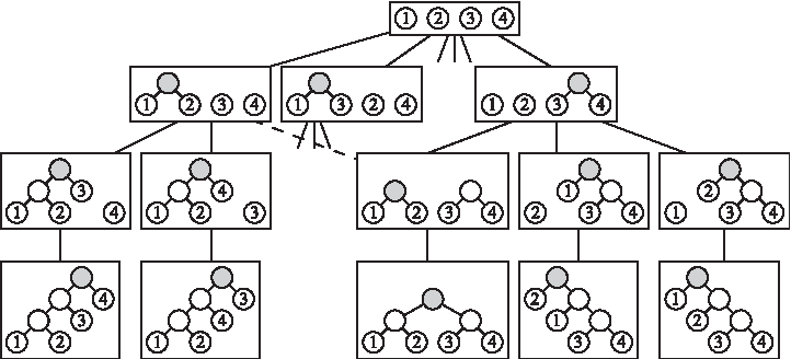Using the definitions above we can define the search space tree \documentclass{aastex}\usepackage{amsbsy}\usepackage{amsfonts}\usepackage{amssymb}\usepackage{bm}\usepackage{mathrsfs}\usepackage{pifont}\usepackage{stmaryrd}\usepackage{textcomp}\usepackage{portland, xspace}\usepackage{amsmath, amsxtra}\pagestyle{empty}\DeclareMathSizes{10}{9}{7}{6}\begin{document} $${ \cal T}_n$$ \end{document} (Fig. 4).

OPEN IN VIEWER

FIG. 4.

An example of the search space tree \documentclass{aastex}\usepackage{amsbsy}\usepackage{amsfonts}\usepackage{amssymb}\usepackage{bm}\usepackage{mathrsfs}\usepackage{pifont}\usepackage{stmaryrd}\usepackage{textcomp}\usepackage{portland, xspace}\usepackage{amsmath, amsxtra}\pagestyle{empty}\DeclareMathSizes{10}{9}{7}{6}\begin{document} $${ \cal T}_4$$ \end{document} . Only some of the nodes of the tree are shown. The dashed line is an edge of \documentclass{aastex}\usepackage{amsbsy}\usepackage{amsfonts}\usepackage{amssymb}\usepackage{bm}\usepackage{mathrsfs}\usepackage{pifont}\usepackage{stmaryrd}\usepackage{textcomp}\usepackage{portland, xspace}\usepackage{amsmath, amsxtra}\pagestyle{empty}\DeclareMathSizes{10}{9}{7}{6}\begin{document} $${ \cal G}_4$$ \end{document} that is not an edge of \documentclass{aastex}\usepackage{amsbsy}\usepackage{amsfonts}\usepackage{amssymb}\usepackage{bm}\usepackage{mathrsfs}\usepackage{pifont}\usepackage{stmaryrd}\usepackage{textcomp}\usepackage{portland, xspace}\usepackage{amsmath, amsxtra}\pagestyle{empty}\DeclareMathSizes{10}{9}{7}{6}\begin{document} $${ \cal T}_4$$ \end{document} . Highlighted in gray within the phylogenies in each node of the search tree are the vertices updated by basic operations when applying our MP approach on \documentclass{aastex}\usepackage{amsbsy}\usepackage{amsfonts}\usepackage{amssymb}\usepackage{bm}\usepackage{mathrsfs}\usepackage{pifont}\usepackage{stmaryrd}\usepackage{textcomp}\usepackage{portland, xspace}\usepackage{amsmath, amsxtra}\pagestyle{empty}\DeclareMathSizes{10}{9}{7}{6}\begin{document} $${ \cal T}_4$$ \end{document} .

Definition 2. The search space tree \documentclass{aastex}\usepackage{amsbsy}\usepackage{amsfonts}\usepackage{amssymb}\usepackage{bm}\usepackage{mathrsfs}\usepackage{pifont}\usepackage{stmaryrd}\usepackage{textcomp}\usepackage{portland, xspace}\usepackage{amsmath, amsxtra}\pagestyle{empty}\DeclareMathSizes{10}{9}{7}{6}\begin{document} $${ \cal T}_n$$ \end{document} is a tree whose nodes are the nodes of \documentclass{aastex}\usepackage{amsbsy}\usepackage{amsfonts}\usepackage{amssymb}\usepackage{bm}\usepackage{mathrsfs}\usepackage{pifont}\usepackage{stmaryrd}\usepackage{textcomp}\usepackage{portland, xspace}\usepackage{amsmath, amsxtra}\pagestyle{empty}\DeclareMathSizes{10}{9}{7}{6}\begin{document} $${ \cal G}_n$$ \end{document} . A node v is the parent of a node u in \documentclass{aastex}\usepackage{amsbsy}\usepackage{amsfonts}\usepackage{amssymb}\usepackage{bm}\usepackage{mathrsfs}\usepackage{pifont}\usepackage{stmaryrd}\usepackage{textcomp}\usepackage{portland, xspace}\usepackage{amsmath, amsxtra}\pagestyle{empty}\DeclareMathSizes{10}{9}{7}{6}\begin{document} $${ \cal T}_n$$ \end{document} if F_v is obtained from F_u by deleting the root of T_u.

The definition above gives an implicit characterization for the children of a node. We now show explicit characterization.

Lemma 2. A node u is a child of a node v in \documentclass{aastex}\usepackage{amsbsy}\usepackage{amsfonts}\usepackage{amssymb}\usepackage{bm}\usepackage{mathrsfs}\usepackage{pifont}\usepackage{stmaryrd}\usepackage{textcomp}\usepackage{portland, xspace}\usepackage{amsmath, amsxtra}\pagestyle{empty}\DeclareMathSizes{10}{9}{7}{6}\begin{document} $${ \cal T}_n$$ \end{document} if and only if F_u is obtained from F_v by merging two trees T₁ and T₂ from F_v with label(T₁) < label(T₂) and either

Proof. (⇒) Let u be a child of v in \documentclass{aastex}\usepackage{amsbsy}\usepackage{amsfonts}\usepackage{amssymb}\usepackage{bm}\usepackage{mathrsfs}\usepackage{pifont}\usepackage{stmaryrd}\usepackage{textcomp}\usepackage{portland, xspace}\usepackage{amsmath, amsxtra}\pagestyle{empty}\DeclareMathSizes{10}{9}{7}{6}\begin{document} $${ \cal T}_n$$ \end{document} . By definition, deleting the root of T_u gives the forest F_v. In other words, if we denote by T₁ and T₂ the two trees formed from T_u by removing its root, then F_u is obtained from F_v by merging T₁ and T₂. Without loss of generality, assume label(T₁) < label(T₂). By definition, label(T_u)=min(label(T₁), label(T₂))=label(T₁). The tree T_u is the non-singleton tree of F_u with minimum label. It follows that in F_u, the leaves with labels \documentclass{aastex}\usepackage{amsbsy}\usepackage{amsfonts}\usepackage{amssymb}\usepackage{bm}\usepackage{mathrsfs}\usepackage{pifont}\usepackage{stmaryrd}\usepackage{textcomp}\usepackage{portland, xspace}\usepackage{amsmath, amsxtra}\pagestyle{empty}\DeclareMathSizes{10}{9}{7}{6}\begin{document} $$1 , \ldots , { \rm label} \ ( T_1 ) - 1$$ \end{document} are each inside a singleton. Since F_u is obtained from F_v by a single merge operation, these leaves are also in singletons in F_v. If T₁ is non-singleton then it is the non-singleton tree in F_v with minimum label(·) value. Thus, T₁=T_v, namely case 1 of the lemma occurs. If T₁ is a singleton then, since the leaves with labels \documentclass{aastex}\usepackage{amsbsy}\usepackage{amsfonts}\usepackage{amssymb}\usepackage{bm}\usepackage{mathrsfs}\usepackage{pifont}\usepackage{stmaryrd}\usepackage{textcomp}\usepackage{portland, xspace}\usepackage{amsmath, amsxtra}\pagestyle{empty}\DeclareMathSizes{10}{9}{7}{6}\begin{document} $$1 , \ldots , { \rm label} \ ( T_1 )$$ \end{document} are in singletons in F_v, we obtain that label(T_v) > label(T₁) and case 2 of the lemma occurs.

(⇐) Suppose F_u is obtained by merging two trees T₁ and T₂ from F_v, and let T′ denote the tree obtained by this merge. In both cases of the lemma we have that the leaves with labels \documentclass{aastex}\usepackage{amsbsy}\usepackage{amsfonts}\usepackage{amssymb}\usepackage{bm}\usepackage{mathrsfs}\usepackage{pifont}\usepackage{stmaryrd}\usepackage{textcomp}\usepackage{portland, xspace}\usepackage{amsmath, amsxtra}\pagestyle{empty}\DeclareMathSizes{10}{9}{7}{6}\begin{document} $$1 , \ldots , { \rm label} \ ( T_1 ) - 1$$ \end{document} are each inside a singleton in F_v, and therefore these leaves are also in singletons in F_u. Therefore, T′ is the non-singleton tree in F_u with minimum label, namely T′=T_u. Thus, v is the parent of u in \documentclass{aastex}\usepackage{amsbsy}\usepackage{amsfonts}\usepackage{amssymb}\usepackage{bm}\usepackage{mathrsfs}\usepackage{pifont}\usepackage{stmaryrd}\usepackage{textcomp}\usepackage{portland, xspace}\usepackage{amsmath, amsxtra}\pagestyle{empty}\DeclareMathSizes{10}{9}{7}{6}\begin{document} $${ \cal T}_n$$ \end{document} .   ■

4. Complexity of the New Search Space

We have proposed a new search method for MP. We now wish to bound the basic operations complexity of our approach. By design, traversing the search space according to our search tree requires performing exactly one basic operation per node; for a node v, the basic operation is applied on the new root of the two merged trees in F_v. Thus, the basic operations complexity is equal to the size of \documentclass{aastex}\usepackage{amsbsy}\usepackage{amsfonts}\usepackage{amssymb}\usepackage{bm}\usepackage{mathrsfs}\usepackage{pifont}\usepackage{stmaryrd}\usepackage{textcomp}\usepackage{portland, xspace}\usepackage{amsmath, amsxtra}\pagestyle{empty}\DeclareMathSizes{10}{9}{7}{6}\begin{document} $${ \cal T}_n$$ \end{document} . We will next show that the size of \documentclass{aastex}\usepackage{amsbsy}\usepackage{amsfonts}\usepackage{amssymb}\usepackage{bm}\usepackage{mathrsfs}\usepackage{pifont}\usepackage{stmaryrd}\usepackage{textcomp}\usepackage{portland, xspace}\usepackage{amsmath, amsxtra}\pagestyle{empty}\DeclareMathSizes{10}{9}{7}{6}\begin{document} $${ \cal T}_n$$ \end{document} is approximately e · (2n−3)!!

Definition 3. Let \documentclass{aastex}\usepackage{amsbsy}\usepackage{amsfonts}\usepackage{amssymb}\usepackage{bm}\usepackage{mathrsfs}\usepackage{pifont}\usepackage{stmaryrd}\usepackage{textcomp}\usepackage{portland, xspace}\usepackage{amsmath, amsxtra}\pagestyle{empty}\DeclareMathSizes{10}{9}{7}{6}\begin{document} $$A_i^n$$ \end{document} denote the number of nodes in level i of \documentclass{aastex}\usepackage{amsbsy}\usepackage{amsfonts}\usepackage{amssymb}\usepackage{bm}\usepackage{mathrsfs}\usepackage{pifont}\usepackage{stmaryrd}\usepackage{textcomp}\usepackage{portland, xspace}\usepackage{amsmath, amsxtra}\pagestyle{empty}\DeclareMathSizes{10}{9}{7}{6}\begin{document} $${ \cal T}_n$$ \end{document} , and let \documentclass{aastex}\usepackage{amsbsy}\usepackage{amsfonts}\usepackage{amssymb}\usepackage{bm}\usepackage{mathrsfs}\usepackage{pifont}\usepackage{stmaryrd}\usepackage{textcomp}\usepackage{portland, xspace}\usepackage{amsmath, amsxtra}\pagestyle{empty}\DeclareMathSizes{10}{9}{7}{6}\begin{document} $$L_{i , k}^n$$ \end{document} denote the number of nodes v in level i for which label(F_v)=k.

Example 1. \documentclass{aastex}\usepackage{amsbsy}\usepackage{amsfonts}\usepackage{amssymb}\usepackage{bm}\usepackage{mathrsfs}\usepackage{pifont}\usepackage{stmaryrd}\usepackage{textcomp}\usepackage{portland, xspace}\usepackage{amsmath, amsxtra}\pagestyle{empty}\DeclareMathSizes{10}{9}{7}{6}\begin{document} $$A_0^n = 1 , \ A_1^n = {n \choose 2}$$ \end{document} , and \documentclass{aastex}\usepackage{amsbsy}\usepackage{amsfonts}\usepackage{amssymb}\usepackage{bm}\usepackage{mathrsfs}\usepackage{pifont}\usepackage{stmaryrd}\usepackage{textcomp}\usepackage{portland, xspace}\usepackage{amsmath, amsxtra}\pagestyle{empty}\DeclareMathSizes{10}{9}{7}{6}\begin{document} $$A_{n - 1}^n = ( 2n - 3 ) !!$$ \end{document} .

Note that for a node v in level i of \documentclass{aastex}\usepackage{amsbsy}\usepackage{amsfonts}\usepackage{amssymb}\usepackage{bm}\usepackage{mathrsfs}\usepackage{pifont}\usepackage{stmaryrd}\usepackage{textcomp}\usepackage{portland, xspace}\usepackage{amsmath, amsxtra}\pagestyle{empty}\DeclareMathSizes{10}{9}{7}{6}\begin{document} $${ \cal T}_n$$ \end{document} , the forest F_v contains n−i trees.

Observation 1 If v is a node in level i then label(F_v) ≤ n−i.

Proof. The forest F_v is obtained from the forest of n singletons by a sequence of i merge operations. At least one merge operation must involve a tree containing a leaf with label at most n−i. Thus, the label of the resulting tree is at most n−i. This tree can participate in other merge operations, which either decrease or do not change the label of the tree. At the end of the merge operations the label of the tree is at most n−i and thus label (F_v) ≤ n−i.   ■

Observation 2  \documentclass{aastex}\usepackage{amsbsy}\usepackage{amsfonts}\usepackage{amssymb}\usepackage{bm}\usepackage{mathrsfs}\usepackage{pifont}\usepackage{stmaryrd}\usepackage{textcomp}\usepackage{portland, xspace}\usepackage{amsmath, amsxtra}\pagestyle{empty}\DeclareMathSizes{10}{9}{7}{6}\begin{document} $$A_i^n = \sum \nolimits_{k = 1}^{n - i} \ L^n_{i , k}$$ \end{document} .

Lemma 3.  \documentclass{aastex}\usepackage{amsbsy}\usepackage{amsfonts}\usepackage{amssymb}\usepackage{bm}\usepackage{mathrsfs}\usepackage{pifont}\usepackage{stmaryrd}\usepackage{textcomp}\usepackage{portland, xspace}\usepackage{amsmath, amsxtra}\pagestyle{empty}\DeclareMathSizes{10}{9}{7}{6}\begin{document} $$L_{i + 1 , k}^n = ( n - i - k ) \sum \nolimits_{l = k}^{n - i} \ L_{i , l}^n$$ \end{document} .

Proof. First, we count the number of children with label k for a node in level i with label l (we will soon show that this number does not depend on the topology of the corresponding forest). Let v be some node in level i with label l. Note that the forests corresponding to the children of v have labels at most l. For a child u of v for which label(F_u)=k, the forest F_u is obtained by merging two trees T₁ and T₂ from F_v such that label(T₁)=k and label(T₂) > k (note that T₁=T_v if k=l, and otherwise T₁ is a singleton). It follows that the number of children of v with label k is the number of trees T in F_v with label(T) > k. Since k ≤ l and the leaves with labels \documentclass{aastex}\usepackage{amsbsy}\usepackage{amsfonts}\usepackage{amssymb}\usepackage{bm}\usepackage{mathrsfs}\usepackage{pifont}\usepackage{stmaryrd}\usepackage{textcomp}\usepackage{portland, xspace}\usepackage{amsmath, amsxtra}\pagestyle{empty}\DeclareMathSizes{10}{9}{7}{6}\begin{document} $$1 , \ldots , l - 1$$ \end{document} are in singletons, it follows that there are exactly k trees with label at most k. The total number of trees in F_v is n−i and therefore F_v contains n−i−k trees with label greater than k. Thus, the number of children of v with label k is n−i−k (not depending on the topology nor on l).

From the above we can deduce a recursive formula for \documentclass{aastex}\usepackage{amsbsy}\usepackage{amsfonts}\usepackage{amssymb}\usepackage{bm}\usepackage{mathrsfs}\usepackage{pifont}\usepackage{stmaryrd}\usepackage{textcomp}\usepackage{portland, xspace}\usepackage{amsmath, amsxtra}\pagestyle{empty}\DeclareMathSizes{10}{9}{7}{6}\begin{document} $$L_{i + 1 , k}^n$$ \end{document} . A node in level i+1 with label k is the child of a node in level i with label l ≥ k The lemma follows.   ■

Lemma 4.  \documentclass{aastex}\usepackage{amsbsy}\usepackage{amsfonts}\usepackage{amssymb}\usepackage{bm}\usepackage{mathrsfs}\usepackage{pifont}\usepackage{stmaryrd}\usepackage{textcomp}\usepackage{portland, xspace}\usepackage{amsmath, amsxtra}\pagestyle{empty}\DeclareMathSizes{10}{9}{7}{6}\begin{document} $$L_{i , k}^n = ( 2i - 1 ) !! \ {n - k + i - 1 \choose 2i - 1}$$ \end{document} .

Proof. We prove the lemma using induction on i. For the base of the induction we need to show that \documentclass{aastex}\usepackage{amsbsy}\usepackage{amsfonts}\usepackage{amssymb}\usepackage{bm}\usepackage{mathrsfs}\usepackage{pifont}\usepackage{stmaryrd}\usepackage{textcomp}\usepackage{portland, xspace}\usepackage{amsmath, amsxtra}\pagestyle{empty}\DeclareMathSizes{10}{9}{7}{6}\begin{document} $$L_{1 , k}^n = n - k$$ \end{document} for all \documentclass{aastex}\usepackage{amsbsy}\usepackage{amsfonts}\usepackage{amssymb}\usepackage{bm}\usepackage{mathrsfs}\usepackage{pifont}\usepackage{stmaryrd}\usepackage{textcomp}\usepackage{portland, xspace}\usepackage{amsmath, amsxtra}\pagestyle{empty}\DeclareMathSizes{10}{9}{7}{6}\begin{document} $$k = 1 , \ldots , n - 1$$ \end{document} . Fix some k. The forest corresponding to a node in level 1 with label k is obtained from the forest of n singletons by merging a singleton with label k with a singleton with label larger than k. Therefore, \documentclass{aastex}\usepackage{amsbsy}\usepackage{amsfonts}\usepackage{amssymb}\usepackage{bm}\usepackage{mathrsfs}\usepackage{pifont}\usepackage{stmaryrd}\usepackage{textcomp}\usepackage{portland, xspace}\usepackage{amsmath, amsxtra}\pagestyle{empty}\DeclareMathSizes{10}{9}{7}{6}\begin{document} $$L^n_{1 , k} = n - k$$ \end{document} .

We now prove the induction step. Assume that the lemma holds for i′ < i. By the induction hypothesis and Lemma 3, \documentclass{aastex}\usepackage{amsbsy}\usepackage{amsfonts}\usepackage{amssymb}\usepackage{bm}\usepackage{mathrsfs}\usepackage{pifont}\usepackage{stmaryrd}\usepackage{textcomp}\usepackage{portland, xspace}\usepackage{amsmath, amsxtra}\pagestyle{empty}\DeclareMathSizes{10}{9}{7}{6}\begin{document} \begin{align*}L^n_{i , k} = ( n - i - k + 1 ) \sum\limits_{l = k}^{n - i + 1}L^n_{i - 1 , l} & = ( n - i - k + 1 ) \sum\limits_{l = k}^{n - i + 1} ( 2i - 3 ) !!{n - l + i - 2 \choose 2i - 3} \\ & = ( n - i - k + 1 ) ( 2i - 3 ) !! \sum\limits_{m = 0}^{n - i - k + 1}{2i - 3 + m \choose 2i - 3}.\end{align*} \end{document}

Using the equality \documentclass{aastex}\usepackage{amsbsy}\usepackage{amsfonts}\usepackage{amssymb}\usepackage{bm}\usepackage{mathrsfs}\usepackage{pifont}\usepackage{stmaryrd}\usepackage{textcomp}\usepackage{portland, xspace}\usepackage{amsmath, amsxtra}\pagestyle{empty}\DeclareMathSizes{10}{9}{7}{6}\begin{document} $$\sum \nolimits_{m = 0}^{n - k} \ {k + m \choose k} = {n + 1 \choose k + 1}$$ \end{document} we obtain \documentclass{aastex}\usepackage{amsbsy}\usepackage{amsfonts}\usepackage{amssymb}\usepackage{bm}\usepackage{mathrsfs}\usepackage{pifont}\usepackage{stmaryrd}\usepackage{textcomp}\usepackage{portland, xspace}\usepackage{amsmath, amsxtra}\pagestyle{empty}\DeclareMathSizes{10}{9}{7}{6}\begin{document} \begin{align*}L^n_{i , k} = ( n - i - k + 1 ) ( 2i - 3 ) !!{n + i - k - 1 \choose 2i - 2} = ( 2i - 1 ) !!{n + i - k - 1 \choose 2i - 1}.\end{align*} \end{document}    ■

Lemma 5.  \documentclass{aastex}\usepackage{amsbsy}\usepackage{amsfonts}\usepackage{amssymb}\usepackage{bm}\usepackage{mathrsfs}\usepackage{pifont}\usepackage{stmaryrd}\usepackage{textcomp}\usepackage{portland, xspace}\usepackage{amsmath, amsxtra}\pagestyle{empty}\DeclareMathSizes{10}{9}{7}{6}\begin{document} $$A_i^n = ( 2i - 1 ) !!{n + i - 1 \choose 2i}$$ \end{document} .

Proof. From Lemma 3 and Observation 2 we have \documentclass{aastex}\usepackage{amsbsy}\usepackage{amsfonts}\usepackage{amssymb}\usepackage{bm}\usepackage{mathrsfs}\usepackage{pifont}\usepackage{stmaryrd}\usepackage{textcomp}\usepackage{portland, xspace}\usepackage{amsmath, amsxtra}\pagestyle{empty}\DeclareMathSizes{10}{9}{7}{6}\begin{document} $$L_{i , 1}^n = ( n - i ) \sum \nolimits_{l = 1}^{n - i + 1} \ L_{i - 1 , l}^n = ( n - i ) A^n_{i - 1}$$ \end{document} . Therefore, \documentclass{aastex}\usepackage{amsbsy}\usepackage{amsfonts}\usepackage{amssymb}\usepackage{bm}\usepackage{mathrsfs}\usepackage{pifont}\usepackage{stmaryrd}\usepackage{textcomp}\usepackage{portland, xspace}\usepackage{amsmath, amsxtra}\pagestyle{empty}\DeclareMathSizes{10}{9}{7}{6}\begin{document} $$A_i^n = \frac { L^n_ { i + 1 , 1 } } { n - i - 1 } $$ \end{document} . By Lemma 4, \documentclass{aastex}\usepackage{amsbsy}\usepackage{amsfonts}\usepackage{amssymb}\usepackage{bm}\usepackage{mathrsfs}\usepackage{pifont}\usepackage{stmaryrd}\usepackage{textcomp}\usepackage{portland, xspace}\usepackage{amsmath, amsxtra}\pagestyle{empty}\DeclareMathSizes{10}{9}{7}{6}\begin{document} $$A_i^n = \frac { ( 2i + 1 ) !! { n + i - 1 \choose 2i + 1 } } { n - i - 1 } = ( 2i - 1 ) !! { n + i - 1 \choose 2i } $$ \end{document} .   ■

Let μ_n be the number of nodes in a search space tree \documentclass{aastex}\usepackage{amsbsy}\usepackage{amsfonts}\usepackage{amssymb}\usepackage{bm}\usepackage{mathrsfs}\usepackage{pifont}\usepackage{stmaryrd}\usepackage{textcomp}\usepackage{portland, xspace}\usepackage{amsmath, amsxtra}\pagestyle{empty}\DeclareMathSizes{10}{9}{7}{6}\begin{document} $${ \cal T}_n$$ \end{document} . Then, \documentclass{aastex}\usepackage{amsbsy}\usepackage{amsfonts}\usepackage{amssymb}\usepackage{bm}\usepackage{mathrsfs}\usepackage{pifont}\usepackage{stmaryrd}\usepackage{textcomp}\usepackage{portland, xspace}\usepackage{amsmath, amsxtra}\pagestyle{empty}\DeclareMathSizes{10}{9}{7}{6}\begin{document} $$\mu_n = \sum \nolimits_{i = 0}^{n - 1} \ A_i^n = \sum \nolimits_{i = 0}^{n - 1} ( 2i - 1 ) !!{n + i - 1 \choose 2i}$$ \end{document} . The series (μ_n) has already been studied, and the following result was obtained (Grosswald, 1978). \documentclass{aastex}\usepackage{amsbsy}\usepackage{amsfonts}\usepackage{amssymb}\usepackage{bm}\usepackage{mathrsfs}\usepackage{pifont}\usepackage{stmaryrd}\usepackage{textcomp}\usepackage{portland, xspace}\usepackage{amsmath, amsxtra}\pagestyle{empty}\DeclareMathSizes{10}{9}{7}{6}\begin{document} \begin{align*}\lim_ { n \to \infty } \frac { \mu_n } { e ( 2n - 3 ) !! } = 1 \tag { 1 } \end{align*} \end{document}

We now compare the size of our search tree to the size of the search tree \documentclass{aastex}\usepackage{amsbsy}\usepackage{amsfonts}\usepackage{amssymb}\usepackage{bm}\usepackage{mathrsfs}\usepackage{pifont}\usepackage{stmaryrd}\usepackage{textcomp}\usepackage{portland, xspace}\usepackage{amsmath, amsxtra}\pagestyle{empty}\DeclareMathSizes{10}{9}{7}{6}\begin{document} $${ \cal T}_n^{{ \rm CSE}}$$ \end{document} . Let η_n be the number of nodes in \documentclass{aastex}\usepackage{amsbsy}\usepackage{amsfonts}\usepackage{amssymb}\usepackage{bm}\usepackage{mathrsfs}\usepackage{pifont}\usepackage{stmaryrd}\usepackage{textcomp}\usepackage{portland, xspace}\usepackage{amsmath, amsxtra}\pagestyle{empty}\DeclareMathSizes{10}{9}{7}{6}\begin{document} $${ \cal T}_n^{{ \rm CSE}}$$ \end{document} . Then, \documentclass{aastex}\usepackage{amsbsy}\usepackage{amsfonts}\usepackage{amssymb}\usepackage{bm}\usepackage{mathrsfs}\usepackage{pifont}\usepackage{stmaryrd}\usepackage{textcomp}\usepackage{portland, xspace}\usepackage{amsmath, amsxtra}\pagestyle{empty}\DeclareMathSizes{10}{9}{7}{6}\begin{document} $$\eta_n = \sum \nolimits_{i = 1}^n ( 2i - 3 ) !!$$ \end{document} . It is easy to verify that \documentclass{aastex}\usepackage{amsbsy}\usepackage{amsfonts}\usepackage{amssymb}\usepackage{bm}\usepackage{mathrsfs}\usepackage{pifont}\usepackage{stmaryrd}\usepackage{textcomp}\usepackage{portland, xspace}\usepackage{amsmath, amsxtra}\pagestyle{empty}\DeclareMathSizes{10}{9}{7}{6}\begin{document} \begin{align*}\lim_ { n \rightarrow \infty } \frac { \eta_n } { ( 2n - 3 ) !! } = 1 \tag { 2 } \end{align*} \end{document}

From Equations (1) and (2) we obtain that \documentclass{aastex}\usepackage{amsbsy}\usepackage{amsfonts}\usepackage{amssymb}\usepackage{bm}\usepackage{mathrsfs}\usepackage{pifont}\usepackage{stmaryrd}\usepackage{textcomp}\usepackage{portland, xspace}\usepackage{amsmath, amsxtra}\pagestyle{empty}\DeclareMathSizes{10}{9}{7}{6}\begin{document} $$\lim_ { n \rightarrow \infty } \ \frac { \mu_n } { \eta_n } = e$$ \end{document} .

Finally, since solving MP using our search tree requires performing exactly one basic operation per node of the search tree, we obtain the following theorem.

Theorem 3. The basic operations complexity for solving MP using the new search space is (1+o(1))·e·(2n−3)!!. Moreover, this complexity is \documentclass{aastex}\usepackage{amsbsy}\usepackage{amsfonts}\usepackage{amssymb}\usepackage{bm}\usepackage{mathrsfs}\usepackage{pifont}\usepackage{stmaryrd}\usepackage{textcomp}\usepackage{portland, xspace}\usepackage{amsmath, amsxtra}\pagestyle{empty}\DeclareMathSizes{10}{9}{7}{6}\begin{document} $$\Theta ( \sqrt{n} )$$ \end{document} times smaller than the complexity of the algorithm of Hendy and Penny.

Proof. The theorem follows from Theorem 2 and Equation (1).   ■

5. Conclusions

We studied the classical problem of exact maximum parsimony (when, in the worst case, all phylogenies need to be enumerated), focusing on the worst case time complexity of various algorithms for the problem.

The first approach we analyzed, proposed by Cavalli-Sforza and Edwards (1967), yields a basic operations complexity of (n−1) · (2n−3)!!. The second approach we analyzed was proposed by Hendy and Penny (1982). Its theoretical worst-case complexity has not been previously analyzed. We showed that the basic operations complexity of this approach is smaller by a factor of \documentclass{aastex}\usepackage{amsbsy}\usepackage{amsfonts}\usepackage{amssymb}\usepackage{bm}\usepackage{mathrsfs}\usepackage{pifont}\usepackage{stmaryrd}\usepackage{textcomp}\usepackage{portland, xspace}\usepackage{amsmath, amsxtra}\pagestyle{empty}\DeclareMathSizes{10}{9}{7}{6}\begin{document} $$\Theta ( \sqrt{n} )$$ \end{document} than the complexity of the Cavalli-Sforza and Edwards approach.

We also proposed a new, faster MP approach, whose basic operations complexity is smaller by a factor of \documentclass{aastex}\usepackage{amsbsy}\usepackage{amsfonts}\usepackage{amssymb}\usepackage{bm}\usepackage{mathrsfs}\usepackage{pifont}\usepackage{stmaryrd}\usepackage{textcomp}\usepackage{portland, xspace}\usepackage{amsmath, amsxtra}\pagestyle{empty}\DeclareMathSizes{10}{9}{7}{6}\begin{document} $$\Theta ( \sqrt{n} )$$ \end{document} than the complexity of the Hendy and Penny approach, and by a factor of Θ(n) than the complexity of the Cavalli-Sforza and Edwards approach. We note that the bound obtained by our proposed algorithm is on the same order of the number of topologies considered by MP, and therefore any approach to exact MP that must enumerate all topologies will not improve our result.

Note that our analysis is done for asymmetrical scoring matrices. When the matrices are symmetrical, the algorithm of Hendy and Penny also achieves a running time of Θ((2n−3)!!) as the traversal to the root is no longer necessary. We emphasize again that this is not the case in practice, and asymmetrical matrices are often used today in various applications of phylogenetics.

Further note that, due to the complexity of MP, when the input data is big it is common in practice to apply either heuristic search or exact optimization methods (such as, for example, branch and bound or intelligent search), in combination with tree-scoring functions, in order to identify a reasonably good tree that fits the data. However, the theoretical questions we ask in this article, even though focused on a linear factor within the complexity of an NP-hard problem, are at the core of the analysis of phylogenetic search. Thus we believe that our results could also be reflected, after further study of appropriate heuristics and search optimizations, to the practical, sparsified search-space solutions applied by current state-of-the-art character-based phylogenetic reconstruction tools.