Fast Flux Module Detection Using Matroid Theory

Abstract

Flux balance analysis (FBA) is one of the most often applied methods on genome-scale metabolic networks. Although FBA uniquely determines the optimal yield, the pathway that achieves this is usually not unique. The analysis of the optimal-yield flux space has been an open challenge. Flux variability analysis is only capturing some properties of the flux space, while elementary mode analysis is intractable due to the enormous number of elementary modes. However, it has been found by Kelk et al. (2012) that the space of optimal-yield fluxes decomposes into flux modules. These decompositions allow a much easier but still comprehensive analysis of the optimal-yield flux space.

Using the mathematical definition of module introduced by Müller and Bockmayr (2013b), we discovered useful connections to matroid theory, through which efficient algorithms enable us to compute the decomposition into modules in a few seconds for genome-scale networks. Using that every module can be represented by one reaction that represents its function, in this article, we also present a method that uses this decomposition to visualize the interplay of modules. We expect the new method to replace flux variability analysis in the pipelines for metabolic networks.

1. Introduction

The metabolic capabilities and behaviors of biological cells are often modeled using metabolic networks. A metabolic network is constituted of a set of chemical compounds and a set of reactions describing the possible transformations of compounds. In the last years it became possible to reconstruct such networks on the genome-scale. This means that on one hand nearly all the reactions that can happen in a biological cell are included. On the other hand such networks consist of thousands of reactions.

Constraint-based methods have proven to be very successful in the analysis of metabolic networks (Papin et al., 2004; Price et al., 2004). In constraint-based methods no detailed information on reaction kinetics is needed. Often, the knowledge of reaction stoichiometries is sufficient. Rows of the stoichiometric matrix correspond to metabolites and columns to reactions: s_ij the i,j-th entry of S is the number of molecules of compound i consumed (s_ij < 0), produced (s_ij > 0), or not involved (s_ij = 0) in reaction j. In steady state this results in linear constraints that express flow conservation on all internal metabolites, with possibly lower and upper bound on fluxes, yielding a polyhedron of feasible flux-vectors P = {v : Sv = 0,ℓ ≤ v ≤ u}.

Among the most prominent analysis methods is flux balance analysis (FBA) (Varma and Palsson, 1994; Orth et al., 2010; Santos et al., 2011). It is, for example, used to compute the optimal biomass yield that can be achieved by a cell under some growth medium (Feist and Palsson, 2010). This amounts to solving a linear programming problem of the form max{cv : v ∈ P}, where cv is the linear function expressing the (weighted) amount of biomass. In general such optimal flows are not unique (Mahadevan and Schilling, 2003). If this is ignored, it can lead to wrong predictions of byproduct flux rates (Khannapho et al., 2008).

Kelk et al. (2012) showed that many reactions have fixed flux rate in all optimal solutions. These are determined by flux variability analysis (FVA) (Burgard et al., 2001; Mahadevan and Schilling, 2003). The remaining variability is due to variability of the fluxes on a number of relatively small subnetworks, which we call flux modules. As an example, we use here an artificial network similar to the one presented by Müller and Bockmayr (2013b) in Figure 1.

FIG. 1.

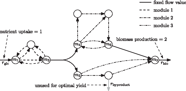
Toy example network. All stoichiometric coefficients are +1, −1, or 0. We assume a fixed nutrient uptake rate of one through r_glc. For optimal biomass production (flux through r_bio) this implies that no side product is produced (flux through r_byproduct is fixed to zero) and an optimal biomass production of two is achieved. The continuous hyperarcs represent reactions carrying fixed flux in all optimal solutions. The modules of the network are marked with different dash styles. Since the reaction r_byproduct carries no flux in any optimal solution, it is grayed out.

In the example, all stoichiometric coefficients are supposed to be +1, −1, or 0. Assuming an input flux rate 1 of the nutrient, any optimum outputs rate 2 of biomass. The continuous hyperarcs represent the reactions that carry fixed flux in any optimal solution. The various dashed sub-hypernetworks indicate the variability present in various optimal solutions. However, for any of the dashed, dash-dotted, or dash-dot-dotted, hypernetworks, we notice that the net influx and the net outflux is the same in every optimal solution: for example in every optimal solution, the dash-dotted subnetwork consumes one unit of metabolite m₄ and produces one unit of metabolite m₆, but there is flexibility in which route this unit flow goes through the dash-dotted network. This allows for seeing a module as one sort of aggregated reaction (see Fig. 2).

FIG. 2.

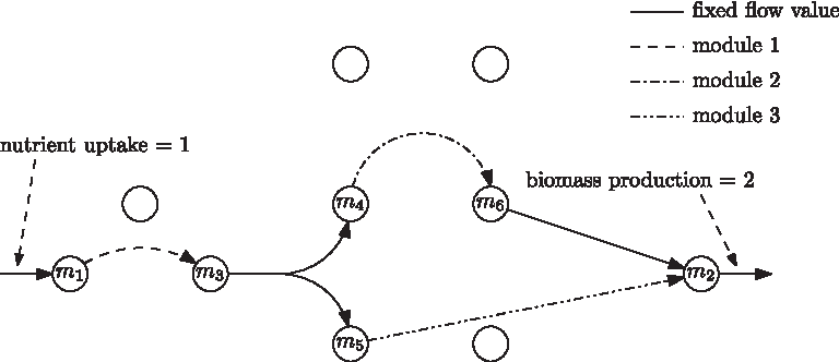
The modules replaced by aggregated reactions.

The fixed input and output compounds of a subnetwork characterizes the notion of flux-module (Müller and Bockmayr, 2013b) in a mathematically rigorous way. Müller and Bockmayr (2013b) showed that every optimal yield elementary flux mode (EFM) (Schuster and Hilgetag, 1994) is a concatenation of reactions with fixed flux and an elementary mode of each of the flux modules. This is illustrated in Figure 3. There are two ways to go through the dashed module, three ways to go through the dash-dotted module, and two ways to go through the dash-dot-dotted module. Hence, 7 subpaths suffice to define the 12 elementary optimal flux modes. Clearly in large networks this combinatorial explosion can be much more dramatic.

FIG. 3.

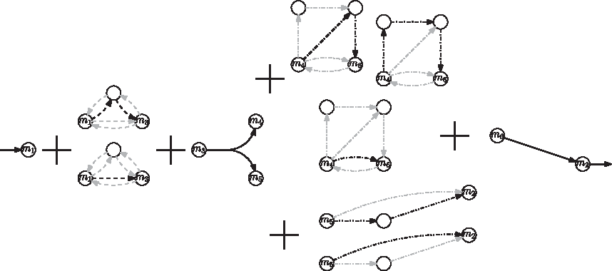
Visualization of all 12 optimal-yield EFMs of the toy network (Fig. 2). By taking one EFM through each module, together with the reactions of fixed nonzero flux, we obtain an optimal yield EFM of the original network. Furthermore, all optimal yield EFMs of the original network can be obtained this way. For each EFM of a module, the used reactions are marked in black, while the unused are marked in gray.

While the method by Kelk et al. (2012) required the enumeration of exponentially many vertices of a flux polyhedron (which are related to the optimal yield EFMs), Müller and Bockmayr (2013b) showed a way to find the modules without needing to compute all extreme solutions. Their method however relied on many runs of FVA. Although faster than EFM enumeration, the method is very sensitive to numerical instabilities, and analyses of genome-scale networks could still take several hours.

The most important result in this article is an extremely simple method allowing to compute the flux-modules in a few seconds for genome-scale metabolic networks. The method, described in section 2, is based on the observation that the modules correspond to the separators of the linear matroid defined by the columns of the stoichiometric matrix that belong to reactions with variable optimal flux. We will explain all these technical concepts in section 2.1. The efficiency of our method is demonstrated in section 3 by application to several genome-scale metabolic networks.

Flux modularity highly depends on the growth conditions. In particular, interesting flux modules can usually only be found in the optimal flux space. Hence, it is of high importance to understand how the decomposition of modules changes under different growth conditions and objective functions. Since with our new method, module computation has become so fast, we can simply compute and compare modules under many different growth conditions and compare the results. Essential for this is a visualization method that shows the interplay of modules in the context of the whole network. In section 2.3 we present a method that automatically generates such a visualization using a clever compression based on flux modules. Results of that method applied to a set of genome-scale metabolic networks can be found in section 3.2.

2. Methods

2.1. Definitions and preliminaries

We use \documentclass{aastex}\usepackage{amsbsy}\usepackage{amsfonts}\usepackage{amssymb}\usepackage{bm}\usepackage{mathrsfs}\usepackage{pifont}\usepackage{stmaryrd}\usepackage{textcomp}\usepackage{portland, xspace}\usepackage{amsmath, amsxtra}\pagestyle{empty}\DeclareMathSizes{10}{9}{7}{6}\begin{document} $${ \cal M}$$ \end{document} to denote the set of metabolites, \documentclass{aastex}\usepackage{amsbsy}\usepackage{amsfonts}\usepackage{amssymb}\usepackage{bm}\usepackage{mathrsfs}\usepackage{pifont}\usepackage{stmaryrd}\usepackage{textcomp}\usepackage{portland, xspace}\usepackage{amsmath, amsxtra}\pagestyle{empty}\DeclareMathSizes{10}{9}{7}{6}\begin{document} $${ \cal R}$$ \end{document} to denote the set of reactions. We abuse the notation for sets also for their size. \documentclass{aastex}\usepackage{amsbsy}\usepackage{amsfonts}\usepackage{amssymb}\usepackage{bm}\usepackage{mathrsfs}\usepackage{pifont}\usepackage{stmaryrd}\usepackage{textcomp}\usepackage{portland, xspace}\usepackage{amsmath, amsxtra}\pagestyle{empty}\DeclareMathSizes{10}{9}{7}{6}\begin{document} $$S \in {\mathbb R}^{{ \cal M} \times { \cal R}}$$ \end{document} denotes the stoichiometric matrix. By appropriate remodeling, the polyhedron P introduced before can be rewritten as \documentclass{aastex}\usepackage{amsbsy}\usepackage{amsfonts}\usepackage{amssymb}\usepackage{bm}\usepackage{mathrsfs}\usepackage{pifont}\usepackage{stmaryrd}\usepackage{textcomp}\usepackage{portland, xspace}\usepackage{amsmath, amsxtra}\pagestyle{empty}\DeclareMathSizes{10}{9}{7}{6}\begin{document} $$P \subseteq \{ v \in {\mathbb R}^{ \cal R} : Sv = b \} $$ \end{document} . We observe that b = 0 leads to the standard steady-state assumption. Here, we also allow b ≠ 0 to simplify notation in the context of modules. Furthermore, the space of optimal-yield fluxes is again a polyhedron and can be written in this form, too (Müller and Bockmayr, 2013b). We will show that we can reduce the analysis of P to the analysis of flux spaces defined by the kernel of \documentclass{aastex}\usepackage{amsbsy}\usepackage{amsfonts}\usepackage{amssymb}\usepackage{bm}\usepackage{mathrsfs}\usepackage{pifont}\usepackage{stmaryrd}\usepackage{textcomp}\usepackage{portland, xspace}\usepackage{amsmath, amsxtra}\pagestyle{empty}\DeclareMathSizes{10}{9}{7}{6}\begin{document} $$S: \ { \rm ker} ( S ) : = \{ v \in {\mathbb R}^{ \cal R} : Sv = 0 \} $$ \end{document} . We use v_r to denote flux through reaction r. The support of flux-vector v is denoted by \documentclass{aastex}\usepackage{amsbsy}\usepackage{amsfonts}\usepackage{amssymb}\usepackage{bm}\usepackage{mathrsfs}\usepackage{pifont}\usepackage{stmaryrd}\usepackage{textcomp}\usepackage{portland, xspace}\usepackage{amsmath, amsxtra}\pagestyle{empty}\DeclareMathSizes{10}{9}{7}{6}\begin{document} $${ \rm supp} ( v ) : = \{ r \in { \cal R} : v_r \neq 0 \} $$ \end{document} . We will conduct FVA for each reaction r of the network by solving the following two linear optimization problems, yielding, respectively, the minimal and maximal possible flux rate: \documentclass{aastex}\usepackage{amsbsy}\usepackage{amsfonts}\usepackage{amssymb}\usepackage{bm}\usepackage{mathrsfs}\usepackage{pifont}\usepackage{stmaryrd}\usepackage{textcomp}\usepackage{portland, xspace}\usepackage{amsmath, amsxtra}\pagestyle{empty}\DeclareMathSizes{10}{9}{7}{6}\begin{document} \begin{align*}\max / \min \{ v_r : Sv = 0 , \ell \leq v \leq u \} \end{align*} \end{document}

We will also be interested in the flux through a subset of reactions \documentclass{aastex}\usepackage{amsbsy}\usepackage{amsfonts}\usepackage{amssymb}\usepackage{bm}\usepackage{mathrsfs}\usepackage{pifont}\usepackage{stmaryrd}\usepackage{textcomp}\usepackage{portland, xspace}\usepackage{amsmath, amsxtra}\pagestyle{empty}\DeclareMathSizes{10}{9}{7}{6}\begin{document} $$A \subseteq { \cal R}$$ \end{document} . Hence, we write v_A to denote the components of v corresponding to the reactions in A, and we use S_A to denote the stoichiometric matrix that only contains the columns corresponding to the reactions in A. We define the projection \documentclass{aastex}\usepackage{amsbsy}\usepackage{amsfonts}\usepackage{amssymb}\usepackage{bm}\usepackage{mathrsfs}\usepackage{pifont}\usepackage{stmaryrd}\usepackage{textcomp}\usepackage{portland, xspace}\usepackage{amsmath, amsxtra}\pagestyle{empty}\DeclareMathSizes{10}{9}{7}{6}\begin{document} $${ \rm pr}_A ( P ) : = \{ v_A : v \in P \} $$ \end{document} .

Definition 1 [flux module, Müller and Bockmayr (2013b)] \documentclass{aastex}\usepackage{amsbsy}\usepackage{amsfonts}\usepackage{amssymb}\usepackage{bm}\usepackage{mathrsfs}\usepackage{pifont}\usepackage{stmaryrd}\usepackage{textcomp}\usepackage{portland, xspace}\usepackage{amsmath, amsxtra}\pagestyle{empty}\DeclareMathSizes{10}{9}{7}{6}\begin{document} $$A \subseteq { \cal R}$$ \end{document} is a P-module if there exists a \documentclass{aastex}\usepackage{amsbsy}\usepackage{amsfonts}\usepackage{amssymb}\usepackage{bm}\usepackage{mathrsfs}\usepackage{pifont}\usepackage{stmaryrd}\usepackage{textcomp}\usepackage{portland, xspace}\usepackage{amsmath, amsxtra}\pagestyle{empty}\DeclareMathSizes{10}{9}{7}{6}\begin{document} $$d \in { \rm R}^{ \cal M}$$ \end{document} s.t. S_Av_A = d for all \documentclass{aastex}\usepackage{amsbsy}\usepackage{amsfonts}\usepackage{amssymb}\usepackage{bm}\usepackage{mathrsfs}\usepackage{pifont}\usepackage{stmaryrd}\usepackage{textcomp}\usepackage{portland, xspace}\usepackage{amsmath, amsxtra}\pagestyle{empty}\DeclareMathSizes{10}{9}{7}{6}\begin{document} $$v \in P$$ \end{document} . We call d the interface flux of the module. ■

In contrast to the definition in Müller and Bockmayr (2013b), we also allow A = ∅ to be a module, which together with \documentclass{aastex}\usepackage{amsbsy}\usepackage{amsfonts}\usepackage{amssymb}\usepackage{bm}\usepackage{mathrsfs}\usepackage{pifont}\usepackage{stmaryrd}\usepackage{textcomp}\usepackage{portland, xspace}\usepackage{amsmath, amsxtra}\pagestyle{empty}\DeclareMathSizes{10}{9}{7}{6}\begin{document} $${ \cal R}$$ \end{document} we call the trivial modules. We present here some useful properties of modules proven in Müller and Bockmayr (2013b). They may also help the reader to get some intuition on the concept of module.

Proposition 1 Properties of Modules.

(i) If disjoint sets A and B are P-modules then A ∪ B is a P-module;

(ii) If A and B are P-modules and B ⊂ A then A\B is a P-module.

The rest of this section is devoted to an introduction to the relevant concepts from Matroid Theory (Oxley, 2011), which is a generalization of graph theory and linear algebra. A matroid is defined by a universe of elements and subsets of them that have some independence structure.

Definition 2 Given a universe \documentclass{aastex}\usepackage{amsbsy}\usepackage{amsfonts}\usepackage{amssymb}\usepackage{bm}\usepackage{mathrsfs}\usepackage{pifont}\usepackage{stmaryrd}\usepackage{textcomp}\usepackage{portland, xspace}\usepackage{amsmath, amsxtra}\pagestyle{empty}\DeclareMathSizes{10}{9}{7}{6}\begin{document} $${ \cal U}$$ \end{document} and a family \documentclass{aastex}\usepackage{amsbsy}\usepackage{amsfonts}\usepackage{amssymb}\usepackage{bm}\usepackage{mathrsfs}\usepackage{pifont}\usepackage{stmaryrd}\usepackage{textcomp}\usepackage{portland, xspace}\usepackage{amsmath, amsxtra}\pagestyle{empty}\DeclareMathSizes{10}{9}{7}{6}\begin{document} $${ \cal A}$$ \end{document} of independent subsets of U, then \documentclass{aastex}\usepackage{amsbsy}\usepackage{amsfonts}\usepackage{amssymb}\usepackage{bm}\usepackage{mathrsfs}\usepackage{pifont}\usepackage{stmaryrd}\usepackage{textcomp}\usepackage{portland, xspace}\usepackage{amsmath, amsxtra}\pagestyle{empty}\DeclareMathSizes{10}{9}{7}{6}\begin{document} $$\{ { \cal U} , { \cal A} \} $$ \end{document} is a matroid if it satisfies the following conditions.

• \documentclass{aastex}\usepackage{amsbsy}\usepackage{amsfonts}\usepackage{amssymb}\usepackage{bm}\usepackage{mathrsfs}\usepackage{pifont}\usepackage{stmaryrd}\usepackage{textcomp}\usepackage{portland, xspace}\usepackage{amsmath, amsxtra}\pagestyle{empty}\DeclareMathSizes{10}{9}{7}{6}\begin{document} $$\emptyset \in { \cal A}$$ \end{document} ;

• If \documentclass{aastex}\usepackage{amsbsy}\usepackage{amsfonts}\usepackage{amssymb}\usepackage{bm}\usepackage{mathrsfs}\usepackage{pifont}\usepackage{stmaryrd}\usepackage{textcomp}\usepackage{portland, xspace}\usepackage{amsmath, amsxtra}\pagestyle{empty}\DeclareMathSizes{10}{9}{7}{6}\begin{document} $$A , A^{ \prime} \in { \cal A}$$ \end{document} , and A′ contains more elements than A, then there exists an element \documentclass{aastex}\usepackage{amsbsy}\usepackage{amsfonts}\usepackage{amssymb}\usepackage{bm}\usepackage{mathrsfs}\usepackage{pifont}\usepackage{stmaryrd}\usepackage{textcomp}\usepackage{portland, xspace}\usepackage{amsmath, amsxtra}\pagestyle{empty}\DeclareMathSizes{10}{9}{7}{6}\begin{document} $$e \in A^{ \prime} \setminus A$$ \end{document} , such that \documentclass{aastex}\usepackage{amsbsy}\usepackage{amsfonts}\usepackage{amssymb}\usepackage{bm}\usepackage{mathrsfs}\usepackage{pifont}\usepackage{stmaryrd}\usepackage{textcomp}\usepackage{portland, xspace}\usepackage{amsmath, amsxtra}\pagestyle{empty}\DeclareMathSizes{10}{9}{7}{6}\begin{document} $$A \cup \{ e \} \in { \cal A}$$ \end{document} . ■

As a very relevant example, a set of vectors in \documentclass{aastex}\usepackage{amsbsy}\usepackage{amsfonts}\usepackage{amssymb}\usepackage{bm}\usepackage{mathrsfs}\usepackage{pifont}\usepackage{stmaryrd}\usepackage{textcomp}\usepackage{portland, xspace}\usepackage{amsmath, amsxtra}\pagestyle{empty}\DeclareMathSizes{10}{9}{7}{6}\begin{document} $${\mathbb R}^{ \cal R}$$ \end{document} , together with their linearly independent subsets form a matroid; a so-called linear matroid. Matroid theory has already been used in the past to describe metabolic networks (Oliveira et al., 2001; Beard et al., 2004). Indeed, many concepts from metabolic networks also exist in matroid theory. For example, if all reactions are reversible (P = ker(S)) then flux modes in metabolic networks correspond to cycles in matroid theory, that is, dependent sets of a matroid. Elementary flux modes correspond to circuits, that is, minimal dependent sets. Notice that in matroid theory we only talk about the support: \documentclass{aastex}\usepackage{amsbsy}\usepackage{amsfonts}\usepackage{amssymb}\usepackage{bm}\usepackage{mathrsfs}\usepackage{pifont}\usepackage{stmaryrd}\usepackage{textcomp}\usepackage{portland, xspace}\usepackage{amsmath, amsxtra}\pagestyle{empty}\DeclareMathSizes{10}{9}{7}{6}\begin{document} $$A \subseteq { \cal R}$$ \end{document} is a cycle if and only if there exists a flux mode \documentclass{aastex}\usepackage{amsbsy}\usepackage{amsfonts}\usepackage{amssymb}\usepackage{bm}\usepackage{mathrsfs}\usepackage{pifont}\usepackage{stmaryrd}\usepackage{textcomp}\usepackage{portland, xspace}\usepackage{amsmath, amsxtra}\pagestyle{empty}\DeclareMathSizes{10}{9}{7}{6}\begin{document} $$v \in { \rm ker} ( S )$$ \end{document} with A = supp(v). Similarly, a circuit \documentclass{aastex}\usepackage{amsbsy}\usepackage{amsfonts}\usepackage{amssymb}\usepackage{bm}\usepackage{mathrsfs}\usepackage{pifont}\usepackage{stmaryrd}\usepackage{textcomp}\usepackage{portland, xspace}\usepackage{amsmath, amsxtra}\pagestyle{empty}\DeclareMathSizes{10}{9}{7}{6}\begin{document} $$C \subseteq { \cal R}$$ \end{document} is a cycle with minimal support.

Matroid theory inherits many powerful concepts from linear algebra like duality and rank (which is important for the proofs displayed in the Supplementary Material, available online at www.liebertpub.com/cmb). Also graph theory introduces some further useful concepts into matroid theory. Important for us is the notion of a connected component of a matroid: two elements of a matroid are in the same component if there exists a circuit that contains both. We notice that in graph theory this property characterizes a two-connected component. A separator of the matroid is now any union of connected components, that is, any of the two sides of a partition of the matroid into two parts A,B such that there exists no circuit intersecting A and B. In section 2.2 we show how the flux modules of a metabolic network correspond one-to-one to the separators of the corresponding matroid. We then use matroid theory to derive a very fast and simple algorithm for finding modules. It is based on a result by Krogdahl (1977). The runtime results on a set of genome-scale metabolic networks are presented in section 3.1.

2.2. Finding modules efficiently

We first show that it is sufficient to analyze modularity as a local property of one point in the inside of the flux space, implying that we can ignore reaction reversibilities and simply analyze a subvector space (Theorem 1). This allows us to describe modularity in terms of matroid separators (Theorem 2), which we then exploit in designing an efficient algorithm to compute modules.

To make the first step, consider a point x inside the flux space and a neighborhood of it (Fig. 4).

FIG. 4.

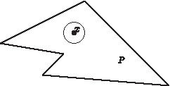
Viewed from a point x inside the flux space, the flux space looks like a linear vector space, and the bounds are not important.

This neighborhood captures all the characteristics needed to analyze modularity of the whole flux space. We only have to deal with the term “inside.” Since \documentclass{aastex}\usepackage{amsbsy}\usepackage{amsfonts}\usepackage{amssymb}\usepackage{bm}\usepackage{mathrsfs}\usepackage{pifont}\usepackage{stmaryrd}\usepackage{textcomp}\usepackage{portland, xspace}\usepackage{amsmath, amsxtra}\pagestyle{empty}\DeclareMathSizes{10}{9}{7}{6}\begin{document} $$P \subseteq \{ v \in {\mathbb R}^{ \cal R} : \, Sv = b \} $$ \end{document} , it follows that P is of lower dimension in \documentclass{aastex}\usepackage{amsbsy}\usepackage{amsfonts}\usepackage{amssymb}\usepackage{bm}\usepackage{mathrsfs}\usepackage{pifont}\usepackage{stmaryrd}\usepackage{textcomp}\usepackage{portland, xspace}\usepackage{amsmath, amsxtra}\pagestyle{empty}\DeclareMathSizes{10}{9}{7}{6}\begin{document} $${\mathbb R}^{ \cal R}$$ \end{document} . Hence, we will only consider the interior relative to ker(S). However, if we have reactions with fixed flux rate, P will also have lower dimension than ker(S). Therefore, we will restrict to reactions with variable flux rate, which we define by: \documentclass{aastex}\usepackage{amsbsy}\usepackage{amsfonts}\usepackage{amssymb}\usepackage{bm}\usepackage{mathrsfs}\usepackage{pifont}\usepackage{stmaryrd}\usepackage{textcomp}\usepackage{portland, xspace}\usepackage{amsmath, amsxtra}\pagestyle{empty}\DeclareMathSizes{10}{9}{7}{6}\begin{document} \begin{align*}V : \, & = \{ r \in { \cal R} : v_r^{ \max} \neq v_r^{ \min} \} , { \rm where} & ( 1 ) \\ v_r^{ \max} :\, & = \sup \{ v_r : v \in P \} \\ v_r^{ \min} : \, & = \inf \{ v_r : v \in P \} \end{align*} \end{document}

This restriction does not destroy the module property:

Observation 1 It holds for all A ⊆ V that A is P-module ⇔ A is pr_V (P)-module.

To guarantee that we can find an x inside the flux space after we restricted to reactions with variable flux rate, we require that P is convex. In a future work we will consider the case of nonconvex flux spaces.

Theorem 1 If \documentclass{aastex}\usepackage{amsbsy}\usepackage{amsfonts}\usepackage{amssymb}\usepackage{bm}\usepackage{mathrsfs}\usepackage{pifont}\usepackage{stmaryrd}\usepackage{textcomp}\usepackage{portland, xspace}\usepackage{amsmath, amsxtra}\pagestyle{empty}\DeclareMathSizes{10}{9}{7}{6}\begin{document} $$P \subseteq \{ v \in {\mathbb R}^{ \cal R} : \, Sv = b \} $$ \end{document} is convex, it holds for all \documentclass{aastex}\usepackage{amsbsy}\usepackage{amsfonts}\usepackage{amssymb}\usepackage{bm}\usepackage{mathrsfs}\usepackage{pifont}\usepackage{stmaryrd}\usepackage{textcomp}\usepackage{portland, xspace}\usepackage{amsmath, amsxtra}\pagestyle{empty}\DeclareMathSizes{10}{9}{7}{6}\begin{document} $$A \subseteq { \cal R}$$ \end{document}

A is P-module ⇔ A ∩ V is ker(S_V )-module.

The proof can be found in the Supplementary Material.

By Theorem 1 we can restrict our attention to the analysis of linear vector spaces. Hence, in the following we will only analyze polyhedra of the form P = ker(S). We will relate modules of ker(S) to separators of the matroid defined by the columns of S. Remember the explanation of a separator in a graph in terms of the nonexistence of a flow circulation in section 2.1 and observe that every module in ker(S) also has interface flux 0 since \documentclass{aastex}\usepackage{amsbsy}\usepackage{amsfonts}\usepackage{amssymb}\usepackage{bm}\usepackage{mathrsfs}\usepackage{pifont}\usepackage{stmaryrd}\usepackage{textcomp}\usepackage{portland, xspace}\usepackage{amsmath, amsxtra}\pagestyle{empty}\DeclareMathSizes{10}{9}{7}{6}\begin{document} $$0 \in$$ \end{document} ker (S).

Formally, we obtain the following theorem, the proof of which is deferred to the Supplementary Material.

Theorem 2 \documentclass{aastex}\usepackage{amsbsy}\usepackage{amsfonts}\usepackage{amssymb}\usepackage{bm}\usepackage{mathrsfs}\usepackage{pifont}\usepackage{stmaryrd}\usepackage{textcomp}\usepackage{portland, xspace}\usepackage{amsmath, amsxtra}\pagestyle{empty}\DeclareMathSizes{10}{9}{7}{6}\begin{document} $$A \subseteq { \cal R}$$ \end{document} is a ker(S)-module if and only if A is a separator in the matroid represented by S. ■

The characterization of modules as separators of matroids allows to compute the flux-modules of a metabolic network efficiently. Since separators and modules are closed under disjoint union, it suffices to describe the set of minimal nontrivial separators (modules).

Definition 3 (Minimal Module) A P-module \documentclass{aastex}\usepackage{amsbsy}\usepackage{amsfonts}\usepackage{amssymb}\usepackage{bm}\usepackage{mathrsfs}\usepackage{pifont}\usepackage{stmaryrd}\usepackage{textcomp}\usepackage{portland, xspace}\usepackage{amsmath, amsxtra}\pagestyle{empty}\DeclareMathSizes{10}{9}{7}{6}\begin{document} $$\emptyset \neq A \subseteq { \cal R}$$ \end{document} is called minimal if there exists no P-module B ≠ ∅ with B ⊂ A. ■

To understand the algorithm for finding the modules, we observe that the minimal nontrivial separators are the connected components of the matroid. Formulated in matroid-terminology we recall from section 2.1 the following characterization of connected components For any two elements (columns of S in the linear matroid, edges in the graph) in the same connected component there exists a circuit that contains them both. For pairs of elements of different connected components this is not true.

We can now build a graph G = (V,E), where V is the set of reactions defined in (1) and there is an edge between two reactions (columns of S_V) if and only if there exists a circuit that contains both. The connected components (in the graph-theoretic sense) of G will be the minimal separators. However, as the number of circuits explodes exponentially, it is not efficient to enumerate all circuits in order to compute the connected components of the graph G. Indeed, this is also not necessary and it suffices to look at a special set of circuits, so-called fundamental circuits (Truemper, 1984).

A set of fundamental circuits is obtained as follows: We start by finding a maximal independent set (also called basis) X of the matroid, which we compute by Algorithm 1. Notice that, starting from the empty set, the algorithm grows X by adding elements only if this keeps X independent. Since we try to add all elements to X, it follows that at the end of the algorithm, X will be a basis of the linear matroid represented by S_V.

Let Y := V \X. Clearly, for every \documentclass{aastex}\usepackage{amsbsy}\usepackage{amsfonts}\usepackage{amssymb}\usepackage{bm}\usepackage{mathrsfs}\usepackage{pifont}\usepackage{stmaryrd}\usepackage{textcomp}\usepackage{portland, xspace}\usepackage{amsmath, amsxtra}\pagestyle{empty}\DeclareMathSizes{10}{9}{7}{6}\begin{document} $$r \in Y$$ \end{document} , adding r to X will create a cycle C^r ⊆ X ∪ {r}. It is easy to see that C^r is actually a circuit, which is called fundamental circuit. In Alg. 1 the fundamental circuits are constructed simultaneously with constructing X. This gives us a so-called partial representation.

We now build, by Algorithm 2, the graph G′ = (V,E′), where two reactions are connected by an edge if there exists a fundamental circuit that contains both. Krogdahl (1977) and Cunningham (1973) showed that the connected components of G′, found by Algorithm 2, are precisely the minimal separators of the matroid.

To each circuit C there exists a flux vector v that is unique up to scaling with C = supp(v), Sv = 0. If we enter for every fundamental circuit the corresponding flux vector as a column into a matrix, we obtain a null-space matrix of S. Hence, this approach can be understood as computing a block-diagonalization of the null-space matrix. Approaches like this in the context of stoichiometric matrices have already been studied in Schuster and Schuster (1991). However, Schuster and Schuster (1991) do not use matroid theory, and it is unclear whether their method will always compute the finest block-diagonalization.

Algorithm 1:

Computes a basis X and its set of fundamental circuits of a matroid represented by S

function ComputePartialRepresentation(S)

\documentclass{aastex}\usepackage{amsbsy}\usepackage{amsfonts}\usepackage{amssymb}\usepackage{bm}\usepackage{mathrsfs}\usepackage{pifont}\usepackage{stmaryrd}\usepackage{textcomp}\usepackage{portland, xspace}\usepackage{amsmath, amsxtra}\pagestyle{empty}\DeclareMathSizes{10}{9}{7}{6}\begin{document} $${ \cal C} = \emptyset$$ \end{document}

for

check feasibility of S_Xv = −S_r

if feasible then

C := supp(v) ∪ {r}

else

X := X ∪ {r}

end if

end for

return

Algorithm 2:

Computes the modules of {v : S_V v = 0}

function ComputeModules()

= ComputePartialRepresentation(S_V)

Build Graph G = {V, E} with

iff there exists

with

= find connected components of G (e.g., using depth-first search).

return

Here we recapitulate all the steps for finding the modules of the optimal flux space of a metabolic network.

1. Determine the optimal value by LP;

2. Set the objective function equal to the optimum value and add it as a constraint;

3. For each reaction r maximize and minimize the flux through r in the optimal flux space;

4. Determine the set V of reactions for which the maximum and the minimum are not equal;

5. Select the set of columns S_V corresponding to V of the stoichiometric matrix S and neglect the non-negativity constraints, i.e., irreversibilities, directions of the reactions;

6. Apply Algorithm 2 to compute the minimal modules \documentclass{aastex}\usepackage{amsbsy}\usepackage{amsfonts}\usepackage{amssymb}\usepackage{bm}\usepackage{mathrsfs}\usepackage{pifont}\usepackage{stmaryrd}\usepackage{textcomp}\usepackage{portland, xspace}\usepackage{amsmath, amsxtra}\pagestyle{empty}\DeclareMathSizes{10}{9}{7}{6}\begin{document} $${ \cal A}$$ \end{document} of \documentclass{aastex}\usepackage{amsbsy}\usepackage{amsfonts}\usepackage{amssymb}\usepackage{bm}\usepackage{mathrsfs}\usepackage{pifont}\usepackage{stmaryrd}\usepackage{textcomp}\usepackage{portland, xspace}\usepackage{amsmath, amsxtra}\pagestyle{empty}\DeclareMathSizes{10}{9}{7}{6}\begin{document} $$\{ v \in {\mathbb R}^V : \, S_V v = 0 \} $$ \end{document} .

7. \documentclass{aastex}\usepackage{amsbsy}\usepackage{amsfonts}\usepackage{amssymb}\usepackage{bm}\usepackage{mathrsfs}\usepackage{pifont}\usepackage{stmaryrd}\usepackage{textcomp}\usepackage{portland, xspace}\usepackage{amsmath, amsxtra}\pagestyle{empty}\DeclareMathSizes{10}{9}{7}{6}\begin{document} $${ \cal A}$$ \end{document} is the set of minimal modules that contain reactions in V . The reactions with fixed flux are all minimal modules by themselves.

We notice that step 3 (and therefore 4) of the algorithm can be parallelized in a trivial way, reducing the computation times even further.

2.3. Visualization

We develop a visualization tool to help us understand how the decomposition of modules changes under different growth conditions and objective functions. By the definition of module, the reactions inside a module have together a fixed function (the interface flux). Hence, we can represent the module by a single reaction with a fixed flux in the genome-scale network. The stoichiometry of the representing reaction is precisely the interface flux of the module.

This way we can create a compressed network that contains all the reactions with fixed flux rates and artificial reactions that represent the modules. This compressed network has the following advantages:

• The number of reactions carrying flux is compressed (a module with many reactions is represented by a single reaction).

• All the reactions in the compressed network have a fixed flux rate.

Unfortunately, the number of fixed reactions is still very large. This prevents automatic visualization of the network and the role of the modules containing variable reactions is obfuscated. However, reactions that have a fixed flux rate can also be grouped together into modules by Proposition 1.

Theoretically, we could group all reactions with a fixed flux rate into one module. This would result in a compressed metabolic network consisting of k + 1 reactions, where k is the number of minimal modules containing reactions with variable flux rates. In particular, the module containing all fixed reactions will likely also contain the biomass- and nutrient-uptake reactions. If we want to understand the role of the modules for biomass production or nutrient uptake, this is not very useful. Moreover, modules of variable reactions may disconnect reactions with fixed flux rates from each other. Such disconnected reactions are important for the mediation between modules and should also be displayed separately. Hence, we decided to build a compressed network as follows:

1. Given: A collection Mod of interesting modules (selected by the user). Mod has to cover all reactions with variable flux rates. Typically Mod contains all minimal modules of variable reactions, a module containing the biomass reaction and modules containing the nutrient uptake reactions.

2. We compute the set \documentclass{aastex}\usepackage{amsbsy}\usepackage{amsfonts}\usepackage{amssymb}\usepackage{bm}\usepackage{mathrsfs}\usepackage{pifont}\usepackage{stmaryrd}\usepackage{textcomp}\usepackage{portland, xspace}\usepackage{amsmath, amsxtra}\pagestyle{empty}\DeclareMathSizes{10}{9}{7}{6}\begin{document} $${ \cal R}_{Mod} \: = \{ r \in { \cal R} : \, r \in M \ \exists \ M \in { Mod} \} $$ \end{document} of reactions in interesting modules.

3. We compute the set \documentclass{aastex}\usepackage{amsbsy}\usepackage{amsfonts}\usepackage{amssymb}\usepackage{bm}\usepackage{mathrsfs}\usepackage{pifont}\usepackage{stmaryrd}\usepackage{textcomp}\usepackage{portland, xspace}\usepackage{amsmath, amsxtra}\pagestyle{empty}\DeclareMathSizes{10}{9}{7}{6}\begin{document} $${ \cal R}_B \: = \{ r \in { \cal R} \setminus { \cal R}_{ Mod} : v_r = 0\ \forall\ v \in P \} $$ \end{document} of blocked reactions.

4. We compute the set \documentclass{aastex}\usepackage{amsbsy}\usepackage{amsfonts}\usepackage{amssymb}\usepackage{bm}\usepackage{mathrsfs}\usepackage{pifont}\usepackage{stmaryrd}\usepackage{textcomp}\usepackage{portland, xspace}\usepackage{amsmath, amsxtra}\pagestyle{empty}\DeclareMathSizes{10}{9}{7}{6}\begin{document} $${ \cal M}_{ Mod} \: = \{ m \in { \cal M} : \exists \ r \ \in { \cal R}_{ Mod} \,\,{\rm such\,\, that}\,\, m \in { \rm supp} ( S_r ) \} $$ \end{document} of metabolites involved in the interesting modules.

5. We consider the metabolic network, where \documentclass{aastex}\usepackage{amsbsy}\usepackage{amsfonts}\usepackage{amssymb}\usepackage{bm}\usepackage{mathrsfs}\usepackage{pifont}\usepackage{stmaryrd}\usepackage{textcomp}\usepackage{portland, xspace}\usepackage{amsmath, amsxtra}\pagestyle{empty}\DeclareMathSizes{10}{9}{7}{6}\begin{document} $${ \cal R}_{ Mod} , \ { \cal R}_{ \rm B}$$ \end{document} , and \documentclass{aastex}\usepackage{amsbsy}\usepackage{amsfonts}\usepackage{amssymb}\usepackage{bm}\usepackage{mathrsfs}\usepackage{pifont}\usepackage{stmaryrd}\usepackage{textcomp}\usepackage{portland, xspace}\usepackage{amsmath, amsxtra}\pagestyle{empty}\DeclareMathSizes{10}{9}{7}{6}\begin{document} $${ \cal M}_{ Mod}$$ \end{document} are removed. It is represented by the stoichiometric matrix \documentclass{aastex}\usepackage{amsbsy}\usepackage{amsfonts}\usepackage{amssymb}\usepackage{bm}\usepackage{mathrsfs}\usepackage{pifont}\usepackage{stmaryrd}\usepackage{textcomp}\usepackage{portland, xspace}\usepackage{amsmath, amsxtra}\pagestyle{empty}\DeclareMathSizes{10}{9}{7}{6}\begin{document} $$S^{ \prime} : = S_{{ \cal M} \backslash { \cal M}_{ Mod} , { \cal R} \backslash ( { \cal R}_{ Mod} \cup { \cal R}_{ B} ) }$$ \end{document} .

6. We compute the connected components Mod_F of S′. We do so by defining the incidence matrix of a bipartite graph, the nodes of which on one side of the bipartition correspond to the rows of S′, and the ones on the other side to the columns of S′, and there is an edge between row-node i and column-node j if and only if \documentclass{aastex}\usepackage{amsbsy}\usepackage{amsfonts}\usepackage{amssymb}\usepackage{bm}\usepackage{mathrsfs}\usepackage{pifont}\usepackage{stmaryrd}\usepackage{textcomp}\usepackage{portland, xspace}\usepackage{amsmath, amsxtra}\pagestyle{empty}\DeclareMathSizes{10}{9}{7}{6}\begin{document} $$S^{ \prime}_{ij} \neq 0$$ \end{document} . The column-nodes represent the reactions in \documentclass{aastex}\usepackage{amsbsy}\usepackage{amsfonts}\usepackage{amssymb}\usepackage{bm}\usepackage{mathrsfs}\usepackage{pifont}\usepackage{stmaryrd}\usepackage{textcomp}\usepackage{portland, xspace}\usepackage{amsmath, amsxtra}\pagestyle{empty}\DeclareMathSizes{10}{9}{7}{6}\begin{document} $${ \cal R} \backslash ( { \cal R}_{ Mod} \cup B )$$ \end{document} , and the corresponding reactions of the connected components of this bipartite graph, whence Mod_F, forms a partition of \documentclass{aastex}\usepackage{amsbsy}\usepackage{amsfonts}\usepackage{amssymb}\usepackage{bm}\usepackage{mathrsfs}\usepackage{pifont}\usepackage{stmaryrd}\usepackage{textcomp}\usepackage{portland, xspace}\usepackage{amsmath, amsxtra}\pagestyle{empty}\DeclareMathSizes{10}{9}{7}{6}\begin{document} $${ \cal R} \backslash ( { \cal R}_{ Mod} \cup B )$$ \end{document} . Clearly, every \documentclass{aastex}\usepackage{amsbsy}\usepackage{amsfonts}\usepackage{amssymb}\usepackage{bm}\usepackage{mathrsfs}\usepackage{pifont}\usepackage{stmaryrd}\usepackage{textcomp}\usepackage{portland, xspace}\usepackage{amsmath, amsxtra}\pagestyle{empty}\DeclareMathSizes{10}{9}{7}{6}\begin{document} $$A \in { Mod}_{{ \rm F}}$$ \end{document} is a module, since Mod_F only contains fixed reactions.

7. We represent each module in Mod, Mod_F by a single reaction with the corresponding interface flux. Let \documentclass{aastex}\usepackage{amsbsy}\usepackage{amsfonts}\usepackage{amssymb}\usepackage{bm}\usepackage{mathrsfs}\usepackage{pifont}\usepackage{stmaryrd}\usepackage{textcomp}\usepackage{portland, xspace}\usepackage{amsmath, amsxtra}\pagestyle{empty}\DeclareMathSizes{10}{9}{7}{6}\begin{document} $${ \cal M}_0$$ \end{document} be the set of metabolites that have a net interface flux of 0 in all these modules. We suppress \documentclass{aastex}\usepackage{amsbsy}\usepackage{amsfonts}\usepackage{amssymb}\usepackage{bm}\usepackage{mathrsfs}\usepackage{pifont}\usepackage{stmaryrd}\usepackage{textcomp}\usepackage{portland, xspace}\usepackage{amsmath, amsxtra}\pagestyle{empty}\DeclareMathSizes{10}{9}{7}{6}\begin{document} $${ \cal M}_0$$ \end{document} since they would just show up as isolated metabolites. We obtain a metabolic network with metabolites \documentclass{aastex}\usepackage{amsbsy}\usepackage{amsfonts}\usepackage{amssymb}\usepackage{bm}\usepackage{mathrsfs}\usepackage{pifont}\usepackage{stmaryrd}\usepackage{textcomp}\usepackage{portland, xspace}\usepackage{amsmath, amsxtra}\pagestyle{empty}\DeclareMathSizes{10}{9}{7}{6}\begin{document} $${ \cal M}^{ \prime} : = { \cal M} \, \backslash \, { \cal M}_0$$ \end{document} and reactions \documentclass{aastex}\usepackage{amsbsy}\usepackage{amsfonts}\usepackage{amssymb}\usepackage{bm}\usepackage{mathrsfs}\usepackage{pifont}\usepackage{stmaryrd}\usepackage{textcomp}\usepackage{portland, xspace}\usepackage{amsmath, amsxtra}\pagestyle{empty}\DeclareMathSizes{10}{9}{7}{6}\begin{document} $${ \cal R}^{ \prime} : =\, { Mod} \cup { Mod}_{ \rm F}$$ \end{document} .

8. We remove reactions disconnected from the network that contain the target reaction, for examples because of modules that form thermodynamically infeasible cycles or otherwise have no role in the metabolism.

In practice, this results in medium-scale networks that can automatically be visualized with graph-drawing software like GraphViz (Gansner and North, 2000).

3. Results

3.1. Runtime of module finding

With the new method we can compute all flux modules for the optimal flux space of genome scale networks in about the same time as is needed for conventional flux variability analysis. In Table 1 we see that the new method using matroid theory outperforms the previous methods in orders of magnitude. We used the metaopt toolbox (Müller and Bockmayr, 2013a) to solve the flux variability subproblems. Unfortunately, we did not have access to all the runtime data of Kelk et al. (2012), which is why some of the data is missing and the reported runtimes may be only from some steps in the pipeline. The computations for the matroid approach were obtained by computations on a four-core desktop computer.

Table 1.

Comparison of Runtimes for Computing Modules in the Optimal Flux Space of Genome Scale Networks

Network	Kelk et al. (2012)	Müller and Bockmayr (2013b)	Using matroids
E. coli iAF1260	133495 sec	755 sec	6.4 sec
E. coli iJR904	1906 sec	162 sec	1.9 sec
E. coli iJO1366			8.4 sec
H. pylori iIT341		55.5 sec	0.8 sec
H. sapiens recon. 1			153.3 sec
H. sapiens recon. 2			1131 sec
M. barkeri iAF692	1088 sec	941 sec	1.4 sec
M. tuberculosis iNJ661	9317 sec	1623 sec	4.3 sec
S. aureus iSB619		127.8 sec	1.2 sec
S. cerevisiae iND750			3.0 sec

In particular, notice that large networks like Human recon 2 can now also be analyzed. In addition, the new method is numerically much more stable. In the method introduced by Müller and Bockmayr (2013b) it often happens that error tolerances are chosen too small or too large, which causes linear programs that should be feasible to be detected as infeasible, etc. This then usually caused the algorithm to abort and the tolerance sometimes needed to be adjusted according to the problem instance.

We experienced that the new matroid-based method is much more robust in this respect. Our initial tolerances of 10⁻²⁰ for the optimization step, 10⁻⁸ for the flux variability, and 10⁻⁹ for the final module computation worked in all cases.

Note that the other two methods are solving slightly different problems. In Müller and Bockmayr (2013b) we were actually looking for modules in the thermodynamically constrained flux space, and in Kelk et al. (2012), rays and linealities are eliminated prior to module computation.

A comparison between the results of Müller and Bockmayr (2013b) and the new method on E. coli iAF1260 revealed that seven of the modules coincide and two modules from the new method contain additional reactions (which have fixed flux under thermodynamic constraints). The remaining modules are computed by the new method but not by Müller and Bockmayr (2013b) since they again only contain reactions that have fixed flux by thermodynamic constraints (usually those modules are formed by a split pair of forward and backward reactions). The differences seem to be small, but a detailed analysis will be subject to future work.

3.2. Visualization

We used the visualization method presented in section 2.3 to create visualizations of the above-mentioned genome scale networks. The results can be found online. In Table 2, we compare the original size of the networks with the size of the compressed networks that are used to visualize the interplay of the flux modules with variable flux rates. Each reaction of the compressed network is a flux module. Every minimal flux module containing reactions with variable flux rates is represented by exactly one reaction. Reactions with fixed flux rate are grouped together. It is interesting to see that although the networks have quite different sizes originally, the compressed sizes do not vary very much.

Table 2.

Size of the Compressed Networks

Network	No. metabolites (original)	No. reactions (original)	No. metabolites (compressed)	No. reactions (compressed)
E. coli iAF1260	1668	2382	46	25
E. coli iJR904	761	1075	42	17
E. coli iJO1366	1805	2583	49	27
H. pylori iIT341	485	554	32	20
M. barkeri iAF692	628	690	35	13
M. tuberculosis iNJ661	826	1025	58	26
S. aureus iSB619	655	743	39	22
S. cerevisiae iND750	1061	1266	57	24

For each of the genome-scale networks a compressed network representing the optimal-yield flux space was computed by compressing flux-modules and sets of reactions with fixed flux to single reactions. All reactions in the compressed network have a unique flux, and the metabolites display the interactions between the flux modules.

Visualizations of some of the example networks and their modules, using the tool dot (Gansner et al., 1993) from the GraphViz toolbox, can be found online. The MATLAB scripts for module detection can be found online as well.

4. Discussion

4.1. Enumeration of optimal-yield pathways

We showed that flux modules (Kelk et al., 2012; Müller and Bockmayr, 2013b) of genome-scale metabolic networks can be computed efficiently using matroids. We confirmed the previous results that the optimal flux space of most genome-scale metabolic networks decomposes into modules. If we want to compute the set of all optimal yield elementary modes, we theoretically can do this by simply computing the optimal yield elementary modes for each module. Then, we can use the decomposition theorem of Müller and Bockmayr (2013b) and obtain all optimal yield elementary modes of the whole network. A small numerical barrier in practice is that EFM enumeration for each module appears to be numerically very unstable. Hence, it is likely that EFMs are missed if not everything is computed using precise rational arithmetic.

We noted that the previous methods (Kelk et al., 2012; Müller and Bockmayr, 2013b) were computing flux modules on slightly different flux spaces [in Kelk et al. (2012) rays and linealities were removed; in Müller and Bockmayr (2013b) we worked on the thermodynamically feasible flux space)]. These differences seem to be small but could be of significant biological importance. For example, it could be that due to thermodynamic constraints a reaction is blocked and hence, we can refine the modules. In a follow-up work we will (mathematically and empirically) analyze the impact of these differences. Also, we want to point out here that, for computing modules, the method by Kelk et al. (2012) has to enumerate all the extreme points of the flux polyhedron of optimal fluxes (after some preprocessing), a much harder task. As a result more information than modules is obtained.

The full flux space is usually not decomposable into modules. In a follow-up article we will generalize the notion of module. This will allow us to find interesting modules also for the full flux space. Furthermore, this will have the potential to derive similar decomposition theorems as in Müller and Bockmayr (2013b) that then will work on the full flux space as well. We think this will be a major step toward EFM enumeration of genome-scale networks.

4.2. Modularity under different growth conditions

It has been observed that the decomposition into modules depends on the growth condition (Kelk et al., 2012; Müller and Bockmayr, 2013b). If we want to understand how the optimal flux space changes if the growth condition is modified, we have to recompute the decomposition into modules. Previously, this was a tedious task. Now it is very simple and fast, and it can be done even for very small changes.

We presented a visualization method that shows the interplay of the modules and how they contribute to optimal biomass production. We think that this visualization will be very helpful to detect when a change in a growth condition significantly changes the structure of the optimal flux space.

For the visualization we use the definition of module to lump reactions together. This way we compute a compressed metabolic network that shows the optimal flux distribution with only a small number of reactions. These networks were small enough to be visualized using automated graph-drawing tools. Currently, we have only little control on how these networks are drawn, causing the visualization to seem to be very sensitive to changes. In particular, it would be interesting if we could get more robust drawing results for small changes in the network.

4.3. Conclusions

In this article we demonstrated the power of matroid theory for metabolic network analysis and used it to present a new method that allows us to compute flux modules very efficiently. This allows us to compute flux modules of many metabolic networks under a large set of different conditions to compare flux modules with existing classical metabolic subsystems like glycolysis.

Compared to classical metabolic subsystems that, at worst, are arbitrary functional groupings of metabolic reactions/species, flux modules are mathematically well defined. They are structural features only depending on a defined set of conditions (inputs, optimality). This qualifies them as a performance and quality metric for genome-scale metabolic networks. Furthermore, it allows us to investigate the modularity, and simplify genome metabolic networks without the risk of a bias from conventional biological interpretation.

Footnotes

Acknowledgments

We thank Timo Maarleveld for providing us with runtime data of the method by Kelk et al. (). This work was supported by the Berlin Mathematical School in form of a PhD stipend and by the Tinbergen Institute.

Author Disclosure Statement

No competing financial interests exist.

Authors' Contributions

A.R. and L.S. found the connection to matroid theory and took care of mathematical correctness. A.R. provided all detailed proofs. L.S. supervised and organized the collaboration process. A.R., F.B., and B.O. developed the visualization method. A.R., L.S., and F.B. worked on the manuscript. All authors read and approved the manuscript.

References

Beard

D.A.

, Babson

, Curtis

, and Qian

2004. Thermodynamic constraints for biochemical networks. J. Theor. Biol., 228, 327–333.

Burgard

A.P.

, Vaidyaraman

, and Maranas

C.D.

2001. Minimal reaction sets for escherichia coli metabolism under different growth requirements and uptake environments. Biotechnology Progress, 17, 791–797.

Cunningham

W.H.

1973. A combinatorial decomposition theory [Ph.D. thesis]. University of Waterloo, Ontario, Canada.

Feist

A.M.

, and Palsson

B.O.

2010. The biomass objective function. Current Opinion in Microbiology, 13, 344–349.

Gansner

E.R.

, Koutsofios

, North

S.C.

, and Vo

K.-p.

1993. A technique for drawing directed graphs. IEEE Transactions on Software Engineering, 19, 214–230.

Gansner

E.R.

, and North

S.C.

2000. An open graph visualization system and its applications to software engineering. Software - Practice and Experience, 30, 1203–1233.

Kelk

S.M.

, Olivier

B.G.

, Stougie

, and Bruggeman

F.J.

2012. Optimal flux spaces of genome-scale stoichiometric models are determined by a few subnetworks. Scientific Reports, 2, 580.

Khannapho

, Zhao

, Bonde

B.L.

, et al. 2008. Selection of objective function in genome scale flux balance analysis for process feed development in antibiotic production. Metabolic Engineering, 10, 227–233.

Krogdahl

1977. The dependence graph for bases in matroids. Discrete Mathematics, 19, 47–59.

10.

Mahadevan

, and Schilling

2003. The effects of alternate optimal solutions in constraint-based genome-scale metabolic models. Metabolic Engineering, 5, 264–276.

11.

Müller

A.C.

, and Bockmayr

2013a. Fast thermodynamically constrainted flux variability analysis. Bioinformatics, 29, 903–909.

12.

Müller

A.C.

, and Bockmayr

2013b. Flux modules in metabolic networks. Journal of Mathematical Biology, 69, 1151–1179.

13.

Oliveira

J.S.

, Bailey

C.G.

, Jones-Oliveira

J.B.

, and Dixon

D.A.

2001. An algebraic-combinatorial model for the identification and mapping of biochemical pathways. Bulletin of Mathematical Biology, 63, 1163–1196.

14.

Orth

J.D.

, Thiele

, and Palsson

B.O.

2010. What is flux balance analysis. Nat. Biotechnol., 28, 245248.

15.

Oxley

2011. Matroid Theory. Oxford Graduate Texts in Mathematics, 2nd ed. Oxford University Press, New York.

16.

Papin

A.J.

, Stelling

, Price

N.D.

, et al. 2004. Comparison of network-based pathway analysis methods. TRENDS in Biotechnology, 22, 400–405.

17.

Price

N.D.

, Reed

J.L.

, and Palsson

B.Ø.

2004. Genome-scale models of microbial cells: evaluating the consequences of constraints. Nature Reviews Microbiology, 2, 886–897.

18.

Santos

, Boele

, and Teusink

2011. A practical guide to genome-scale metabolic models and their analysis. Methods in Enzymology, 500, 509.

19.

Schuster

, and Hilgetag

1994. On elementary flux modes in biochemical systems at steady state. J. Biol. Systems, 2, 165–182.

20.

Schuster

, and Schuster

1991. Detecting strictly detailed balanced subnetworks in open chemical reaction networks. J. Math. Chem., 6, 17–40.

21.

Truemper

1984. Partial matroid representations. European Journal of Combinatorics, 5, 377–394.

22.

Varma

, and Palsson

B.O.

1994. Metabolic flux balancing: Basic concepts, scientific and practical use. Nat. Biotechnol., 12, 994–998.

Supplementary Material

Please find the following supplemental material available below.

For Open Access articles published under a Creative Commons License, all supplemental material carries the same license as the article it is associated with.

For non-Open Access articles published, all supplemental material carries a non-exclusive license, and permission requests for re-use of supplemental material or any part of supplemental material shall be sent directly to the copyright owner as specified in the copyright notice associated with the article.

0.00 MB

0.08 MB