W hats H ap : Weighted Haplotype Assembly for Future-Generation Sequencing Reads

Abstract

The human genome is diploid, which requires assigning heterozygous single nucleotide polymorphisms (SNPs) to the two copies of the genome. The resulting haplotypes, lists of SNPs belonging to each copy, are crucial for downstream analyses in population genetics. Currently, statistical approaches, which are oblivious to direct read information, constitute the state-of-the-art. Haplotype assembly, which addresses phasing directly from sequencing reads, suffers from the fact that sequencing reads of the current generation are too short to serve the purposes of genome-wide phasing

While future-technology sequencing reads will contain sufficient amounts of SNPs per read for phasing, they are also likely to suffer from higher sequencing error rates. Currently, no haplotype assembly approaches exist that allow for taking both increasing read length and sequencing error information into account

Here, we suggest WhatsHap, the first approach that yields provably optimal solutions to the weighted minimum error correction problem in runtime linear in the number of SNPs. WhatsHap is a fixed parameter tractable (FPT) approach with coverage as the parameter. We demonstrate that WhatsHap can handle datasets of coverage up to 20×, and that 15× are generally enough for reliably phasing long reads, even at significantly elevated sequencing error rates. We also find that the switch and flip error rates of the haplotypes we output are favorable when comparing them with state-of-the-art statistical phasers

1. Introduction

The human genome is diploid, that is, each of its autosomes (nonsex chromosomes) comes in two copies. These parental copies are affected by different single nucleotide polymorphisms (SNPs). Assigning the variants to the copies is an instrumental step in evolutionary genomics and genetics, as it allows to, for example, identify selective pressures and subpopulations in population studies (The 1000 Genomes Project Consortium, 2010; Francioli et al., 2014), and to link possibly disease-causing SNPs with one another (Hartl and Clark, 2007). The corresponding assignment process is referred to as phasing and the resulting groups of SNPs are called haplotypes. In the meantime, globally concerted efforts have generated reference panels of haplotypes, for various populations, which may serve corresponding downstream analyses (The International HapMap Consortium, 2007, 2010).

There are two major approaches to phasing variants. The first class of approaches relies on genotypes as input, which are lists of SNP alleles, together with their zygosity status. While homozygous alleles show on both chromosomal copies, and obviously apply for both haplotypes, heterozygous alleles show on only one of the copies and have to be partitioned into two groups. For m heterozygous SNP positions there are thus 2^m many possible haplotypes. The corresponding approaches are usually statistical in nature, and they integrate existing reference panels. The underlying assumption is that the haplotypes to be computed are a mosaic of reference haplotype blocks that arises from recombination during meiosis. The output is the statistically most likely mosaic, given the observed genotypes. Most prevalent approaches are based on latent variable modeling (Howie et al., 2009; Li et al., 2010; Scheet and Stephens, 2006). Other approaches use Markov chain Monte Carlo techniques (Menelaou and Marchini, 2013).

The other class of approaches uses sequencing read data directly. Such approaches virtually assemble reads from identical chromosomal copies and are referred to as haplotype assembly approaches. Following the parsimony principle, the goal is to compute two haplotypes to which one can assign all reads with the least amount of sequencing errors to be corrected and/or erroneous reads to be removed. Among such formulations, the minimum error correction (MEC) problem has gained most of the recent attention. The MEC problem, which we will formally define in section 2, consists in finding the minimum number of corrections to be made to the sequenced nucleotides in order to arrange the reads into two haplotypes without conflicts. A major advantage of MEC is that it can be easily adapted to a weighted version (wMEC) in order to deal with phred-scaled error probabilities. Such phred-based error schemes are vital, in particular for processing long reads generated by future technologies, as these are prone to elevated sequencing error rates. An optimal solution for the wMEC problem then translates to a maximum likelihood scenario relative to the errors to be corrected.

In tera-scale sequencing projects (e.g., Boomsma et al., 2013; The 1000 Genomes Project Consortium, 2010), ever increasing read length and decreasing sequencing cost make it clearly desirable to phase directly from read data. However, statistical approaches are still the methodology of choice because (i) most NGS reads are still too short to bridge so-called variant deserts. Successful read-based phasing, however, requires that all pairs of neighboring heterozygous SNP alleles are covered; and (ii) the MEC problem is \documentclass{aastex}\usepackage{amsbsy}\usepackage{amsfonts}\usepackage{amssymb}\usepackage{bm}\usepackage{mathrsfs}\usepackage{pifont}\usepackage{stmaryrd}\usepackage{textcomp}\usepackage{portland, xspace}\usepackage{amsmath, amsxtra}\pagestyle{empty}\DeclareMathSizes {10} {9} {7} {6} \begin{document} $${ \cal NP}$$ \end{document} -hard, and so are all other similar problem formulations.

Most advanced existing algorithmic solutions to MEC (Chen et al., 2013; He et al., 2010) ironically often benefit precisely from variant deserts, because these allow for decomposing a problem instance into independent parts. A major motivation behind read-based approaches, however, is to handle long reads that cover as many variants as possible, thereby bridging all variant deserts. Hence, the current perception of haplotype assembly is often that it underlies theoretical limitations that are too hard to overcome.

Here, we present WhatsHap, a fixed parameter tractable (FPT) approach to wMEC where coverage, that is the number of fragments that cover an SNP position, is the only parameter. Hence, the runtime of our approach is polynomial (in fact, linear) in the number of SNPs. A linear-runtime solution for the wMEC addresses both that future sequencing technologies generate reads of tens of thousands of base pairs (bp), and that those will likely suffer from elevated sequencing error rates. A carefully engineered implementation of our algorithm allows the treatment of whole-genome datasets of maximum coverage up to 20× on the order of hours on a standard workstation. For datasets of higher coverage, we provide a technique for choosing a reasonable selection of reads. We compare and evaluate WhatsHap in a variety of aspects, based on simulated reads of various lengths, all of which stem from a true genome (Levy et al., 2007). We show that coverage rates of 10–15× are sufficient for achieving low phasing error rates in haplotype assembly. We demonstrate that in comparison to state-of-the-art haplotype assembly approaches, WhatsHap has favorable runtime, in particular on data sets of 10–15× coverage, which is the critical coverage rate. We further demonstrate that the haplotypes computed by WhatsHap only suffer from minor amounts of errors. It may be noteworthy that error rates are quite favorable also in comparison with statistical phasing approaches, which still constitute the practical state-of-the-art.

2. The Weighted Minimum Error Correction Problem

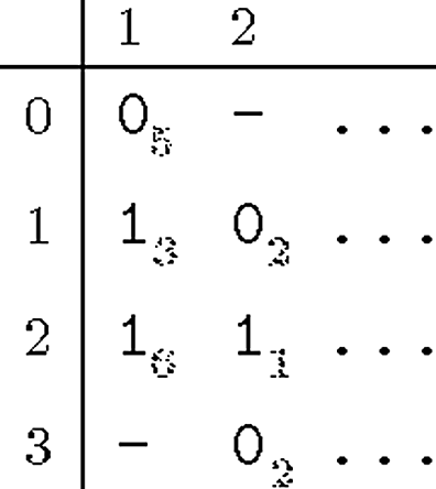
The input to the MEC problem is a matrix \documentclass{aastex}\usepackage{amsbsy}\usepackage{amsfonts}\usepackage{amssymb}\usepackage{bm}\usepackage{mathrsfs}\usepackage{pifont}\usepackage{stmaryrd}\usepackage{textcomp}\usepackage{portland, xspace}\usepackage{amsmath, amsxtra}\pagestyle{empty}\DeclareMathSizes {10} {9} {7} {6} \begin{document} $${ \cal F}$$ \end{document} with entries in {0, 1,−}. Each row of \documentclass{aastex}\usepackage{amsbsy}\usepackage{amsfonts}\usepackage{amssymb}\usepackage{bm}\usepackage{mathrsfs}\usepackage{pifont}\usepackage{stmaryrd}\usepackage{textcomp}\usepackage{portland, xspace}\usepackage{amsmath, amsxtra}\pagestyle{empty}\DeclareMathSizes {10} {9} {7} {6} \begin{document} $${ \cal F}$$ \end{document} corresponds to a fragment/read. Each column of \documentclass{aastex}\usepackage{amsbsy}\usepackage{amsfonts}\usepackage{amssymb}\usepackage{bm}\usepackage{mathrsfs}\usepackage{pifont}\usepackage{stmaryrd}\usepackage{textcomp}\usepackage{portland, xspace}\usepackage{amsmath, amsxtra}\pagestyle{empty}\DeclareMathSizes {10} {9} {7} {6} \begin{document} $${ \cal F}$$ \end{document} corresponds to an SNP position. The “−” symbol, which is referred to as a hole, is used when a fragment does not contain any information at the corresponding SNP position. This can be either because the SNP position is not covered by the read, or because the read gives no accurate information at that position. Let n be the number of rows (or fragments) of \documentclass{aastex}\usepackage{amsbsy}\usepackage{amsfonts}\usepackage{amssymb}\usepackage{bm}\usepackage{mathrsfs}\usepackage{pifont}\usepackage{stmaryrd}\usepackage{textcomp}\usepackage{portland, xspace}\usepackage{amsmath, amsxtra}\pagestyle{empty}\DeclareMathSizes {10} {9} {7} {6} \begin{document} $${ \cal F}$$ \end{document} and m the number of columns (or SNP positions).

A haplotype can formally be defined as a string of length m consisting of 0's and 1's. If h is a haplotype, then the i-th row of \documentclass{aastex}\usepackage{amsbsy}\usepackage{amsfonts}\usepackage{amssymb}\usepackage{bm}\usepackage{mathrsfs}\usepackage{pifont}\usepackage{stmaryrd}\usepackage{textcomp}\usepackage{portland, xspace}\usepackage{amsmath, amsxtra}\pagestyle{empty}\DeclareMathSizes {10} {9} {7} {6} \begin{document} $${ \cal F}$$ \end{document} is said to conflict with h if there is some SNP position j for which \documentclass{aastex}\usepackage{amsbsy}\usepackage{amsfonts}\usepackage{amssymb}\usepackage{bm}\usepackage{mathrsfs}\usepackage{pifont}\usepackage{stmaryrd}\usepackage{textcomp}\usepackage{portland, xspace}\usepackage{amsmath, amsxtra}\pagestyle{empty}\DeclareMathSizes {10} {9} {7} {6} \begin{document} $$h ( j ) \neq{ \cal F} ( i , j )$$ \end{document} while \documentclass{aastex}\usepackage{amsbsy}\usepackage{amsfonts}\usepackage{amssymb}\usepackage{bm}\usepackage{mathrsfs}\usepackage{pifont}\usepackage{stmaryrd}\usepackage{textcomp}\usepackage{portland, xspace}\usepackage{amsmath, amsxtra}\pagestyle{empty}\DeclareMathSizes {10} {9} {7} {6} \begin{document} $${ \cal F} ( i , j ) \neq -$$ \end{document} . We say that \documentclass{aastex}\usepackage{amsbsy}\usepackage{amsfonts}\usepackage{amssymb}\usepackage{bm}\usepackage{mathrsfs}\usepackage{pifont}\usepackage{stmaryrd}\usepackage{textcomp}\usepackage{portland, xspace}\usepackage{amsmath, amsxtra}\pagestyle{empty}\DeclareMathSizes {10} {9} {7} {6} \begin{document} $${ \cal F}$$ \end{document} is conflict free if there exist two haplotypes h₁, h₂ such that each row of \documentclass{aastex}\usepackage{amsbsy}\usepackage{amsfonts}\usepackage{amssymb}\usepackage{bm}\usepackage{mathrsfs}\usepackage{pifont}\usepackage{stmaryrd}\usepackage{textcomp}\usepackage{portland, xspace}\usepackage{amsmath, amsxtra}\pagestyle{empty}\DeclareMathSizes {10} {9} {7} {6} \begin{document} $${ \cal F}$$ \end{document} does not conflict with at least one of h₁ and h₂. Under the all-heterozygous assumption, where all columns correspond to heterozygous sites, h₁ must be the complement of h₂. Some methods need to make this assumption for computational reasons, and this is why we mention it, although our tool does not need it.

The goal of MEC is to make \documentclass{aastex}\usepackage{amsbsy}\usepackage{amsfonts}\usepackage{amssymb}\usepackage{bm}\usepackage{mathrsfs}\usepackage{pifont}\usepackage{stmaryrd}\usepackage{textcomp}\usepackage{portland, xspace}\usepackage{amsmath, amsxtra}\pagestyle{empty}\DeclareMathSizes {10} {9} {7} {6} \begin{document} $${ \cal F}$$ \end{document} conflict free by flipping a minimum number of entries of \documentclass{aastex}\usepackage{amsbsy}\usepackage{amsfonts}\usepackage{amssymb}\usepackage{bm}\usepackage{mathrsfs}\usepackage{pifont}\usepackage{stmaryrd}\usepackage{textcomp}\usepackage{portland, xspace}\usepackage{amsmath, amsxtra}\pagestyle{empty}\DeclareMathSizes {10} {9} {7} {6} \begin{document} $${ \cal F}$$ \end{document} from 0 to 1 or vice versa. The weighted variant of MEC, denoted wMEC, has an additional weight function w as input. This weight function assigns a non-negative weight w(i, j) to each entry \documentclass{aastex}\usepackage{amsbsy}\usepackage{amsfonts}\usepackage{amssymb}\usepackage{bm}\usepackage{mathrsfs}\usepackage{pifont}\usepackage{stmaryrd}\usepackage{textcomp}\usepackage{portland, xspace}\usepackage{amsmath, amsxtra}\pagestyle{empty}\DeclareMathSizes {10} {9} {7} {6} \begin{document} $${ \cal F} ( i , j )$$ \end{document} of \documentclass{aastex}\usepackage{amsbsy}\usepackage{amsfonts}\usepackage{amssymb}\usepackage{bm}\usepackage{mathrsfs}\usepackage{pifont}\usepackage{stmaryrd}\usepackage{textcomp}\usepackage{portland, xspace}\usepackage{amsmath, amsxtra}\pagestyle{empty}\DeclareMathSizes {10} {9} {7} {6} \begin{document} $${ \cal F}$$ \end{document} . This weight can reflect the relative confidence that the entry is correctly sequenced. The goal of wMEC is to make \documentclass{aastex}\usepackage{amsbsy}\usepackage{amsfonts}\usepackage{amssymb}\usepackage{bm}\usepackage{mathrsfs}\usepackage{pifont}\usepackage{stmaryrd}\usepackage{textcomp}\usepackage{portland, xspace}\usepackage{amsmath, amsxtra}\pagestyle{empty}\DeclareMathSizes {10} {9} {7} {6} \begin{document} $${ \cal F}$$ \end{document} conflict free by flipping entries in \documentclass{aastex}\usepackage{amsbsy}\usepackage{amsfonts}\usepackage{amssymb}\usepackage{bm}\usepackage{mathrsfs}\usepackage{pifont}\usepackage{stmaryrd}\usepackage{textcomp}\usepackage{portland, xspace}\usepackage{amsmath, amsxtra}\pagestyle{empty}\DeclareMathSizes {10} {9} {7} {6} \begin{document} $${ \cal F}$$ \end{document} with a minimum total weight.

The MEC problem, which is also called minimum letter flip, was introduced by Lippert et al. (2002). Cilibrasi et al. (2005) showed that this problem is NP-hard even if each fragment is “gapless,” that is, if it consists of a consecutive sequence of 0's and 1's with holes to the left and to the right. Panconesi and Sozio (2004) were the first to propose a practical heuristic for solving MEC. An exact branch and bound algorithm and a heuristic genetic algorithm were presented by Wang et al. (2005). Levy et al. (2007) designed a greedy heuristic to assemble the haplotype of the genome of J. Craig Venter. Bansal et al. (2008) developed an MCMC method to sample a set of likely haplotypes. In a follow-up, some of the authors proposed a much faster MAX-CUT-based heuristic algorithm called HapCUT (Bansal and Bafna, 2008), which they show to outperform (Panconesi and Sozio, 2004; Levy et al., 2007), while showing similar accuracy to (Bansal et al., 2008) in shorter running time. Very recently, Selvaraj et al. (2013) combined the HapCUT (Bansal and Bafna, 2008) algorithm with proximity-ligation, which exploits information from “chromosome territories,” to develop a method that reports good results on whole-genome haplotype reconstruction. He et al. (2010) proposed an exact dynamic programming algorithm. However, their algorithm depends exponentially on the length of the longest read, which means that for practical data this method has to ignore all long reads. Aguiar and Istrail (2012, 2013) suggested a heuristic approach for MEC, which they show to perform well compared to previous methods. Exact integer linear programming (ILP)–based approaches were proposed by Fouilhoux and Mahjoub (2012) and Chen et al. (2013). Both methods have difficulties solving practical instances optimally in a reasonable amount of time. Chen et al. (2013), for instance, report that they need 31 hours (resp., 12 days) to solve the HuRef data set with (resp., without) the all-heterozygous assumption. For this reason, Chen et al. (2013) also propose a heuristic for solving difficult subproblems. Deng et al. (2013) suggested a different dynamic programming algorithm for MEC, which is exponential in the maximum coverage of an SNP.

The weighted variant of MEC was first suggested by Greenberg et al. (2004). Zhao et al. (2005) proposed a heuristic for a special case of wMEC and presented experiments showing that wMEC is more accurate than MEC. In the next section, we presented a dynamic programming algorithm for wMEC, which is similar in spirit to the approach of Deng et al. (2013), but extends it to the weighted case and broadens its applicability using techniques from algorithm engineering.

3. A Dynamic Programming Algorithm for Wmec

We now present the WhatsHap algorithm for solving wMEC. WhatsHap is an exact dynamic programming approach that solves wMEC instances in linear time if we assume bounded coverage.

Consider the input matrix \documentclass{aastex}\usepackage{amsbsy}\usepackage{amsfonts}\usepackage{amssymb}\usepackage{bm}\usepackage{mathrsfs}\usepackage{pifont}\usepackage{stmaryrd}\usepackage{textcomp}\usepackage{portland, xspace}\usepackage{amsmath, amsxtra}\pagestyle{empty}\DeclareMathSizes {10} {9} {7} {6} \begin{document} $${ \cal F}$$ \end{document} of the wMEC problem. Each entry \documentclass{aastex}\usepackage{amsbsy}\usepackage{amsfonts}\usepackage{amssymb}\usepackage{bm}\usepackage{mathrsfs}\usepackage{pifont}\usepackage{stmaryrd}\usepackage{textcomp}\usepackage{portland, xspace}\usepackage{amsmath, amsxtra}\pagestyle{empty}\DeclareMathSizes {10} {9} {7} {6} \begin{document} $${ \cal F} ( i , j ) \neq -$$ \end{document} is associated with a confidence degree w(i, j) telling how likely it is that \documentclass{aastex}\usepackage{amsbsy}\usepackage{amsfonts}\usepackage{amssymb}\usepackage{bm}\usepackage{mathrsfs}\usepackage{pifont}\usepackage{stmaryrd}\usepackage{textcomp}\usepackage{portland, xspace}\usepackage{amsmath, amsxtra}\pagestyle{empty}\DeclareMathSizes {10} {9} {7} {6} \begin{document} $${ \cal F} ( i , j )$$ \end{document} is correctly sequenced and that its fragment i is correctly mapped to location j. We use such values as a weight for the correction we need to minimize in the wMEC model. When these weights are log-likelihoods, summing them up corresponds to multiplying probabilities and, thus, finding a minimum weight solution corresponds to finding a maximum likelihood bipartition of the reads/fragments.

Our dynamic programming (DP) formulation is based on the observation that, for each column, only active fragments need to be considered; a fragment i is said to be active in every column j that lies in between its leftmost nonhole entry and its rightmost nonhole entry. Thus, paired-end reads remain active in the “internal segment” between the two reads. Let F(j) be the set of fragments that are active at SNP position j and let F be the set of all fragments. The aim is to find a bipartition (R*, S*) of F such that the changes in R* and S* to make \documentclass{aastex}\usepackage{amsbsy}\usepackage{amsfonts}\usepackage{amssymb}\usepackage{bm}\usepackage{mathrsfs}\usepackage{pifont}\usepackage{stmaryrd}\usepackage{textcomp}\usepackage{portland, xspace}\usepackage{amsmath, amsxtra}\pagestyle{empty}\DeclareMathSizes {10} {9} {7} {6} \begin{document} $${ \cal F}$$ \end{document} conflict-free have minimum total weight.

Proceeding columnwise from SNP position 1 to m, our approach computes a DP table column C(j,·) for each \documentclass{aastex}\usepackage{amsbsy}\usepackage{amsfonts}\usepackage{amssymb}\usepackage{bm}\usepackage{mathrsfs}\usepackage{pifont}\usepackage{stmaryrd}\usepackage{textcomp}\usepackage{portland, xspace}\usepackage{amsmath, amsxtra}\pagestyle{empty}\DeclareMathSizes {10} {9} {7} {6} \begin{document} $$j \in \{ 1 , \ldots , m \} $$ \end{document} . We say that a bipartition B′=(R′, S′) of all fragments F extends bipartition B=(R, S) of F(j), if R ⊆ R′ and S ⊆ S′. We define \documentclass{aastex}\usepackage{amsbsy}\usepackage{amsfonts}\usepackage{amssymb}\usepackage{bm}\usepackage{mathrsfs}\usepackage{pifont}\usepackage{stmaryrd}\usepackage{textcomp}\usepackage{portland, xspace}\usepackage{amsmath, amsxtra}\pagestyle{empty}\DeclareMathSizes {10} {9} {7} {6} \begin{document} $${ \cal B} ( X )$$ \end{document} to be the set of all bipartitions of X. Given a bipartition (R, S), we denote \documentclass{aastex}\usepackage{amsbsy}\usepackage{amsfonts}\usepackage{amssymb}\usepackage{bm}\usepackage{mathrsfs}\usepackage{pifont}\usepackage{stmaryrd}\usepackage{textcomp}\usepackage{portland, xspace}\usepackage{amsmath, amsxtra}\pagestyle{empty}\DeclareMathSizes {10} {9} {7} {6} \begin{document} $${ \cal B} ( X \mid ( R , S ) )$$ \end{document} the set of all bipartitions of X that extend (R, S), that is, \documentclass{aastex}\usepackage{amsbsy}\usepackage{amsfonts}\usepackage{amssymb}\usepackage{bm}\usepackage{mathrsfs}\usepackage{pifont}\usepackage{stmaryrd}\usepackage{textcomp}\usepackage{portland,xspace}\usepackage{amsmath,amsxtra}\pagestyle{empty}\DeclareMathSizes{10}{9}{7}{6} \begin{document} \begin{align*}{ \cal B} ( X \mid ( R , S ) ) \,{:} = \{ ( R^{ \prime} , S^{ \prime} ) \in { \cal B} ( X ) \mid R \subseteq R^{ \prime} \ { \rm and} \ S \subseteq S^{ \prime} \} .\end{align*} \end{document}

The basic idea of our dynamic program is as follows: for every bipartition B=(R, S) of F(j), entry C(j, B) gives the minimum cost of a bipartition of all fragments F that renders positions \documentclass{aastex}\usepackage{amsbsy}\usepackage{amsfonts}\usepackage{amssymb}\usepackage{bm}\usepackage{mathrsfs}\usepackage{pifont}\usepackage{stmaryrd}\usepackage{textcomp}\usepackage{portland, xspace}\usepackage{amsmath, amsxtra}\pagestyle{empty}\DeclareMathSizes {10} {9} {7} {6} \begin{document} $$1 , \ldots , j$$ \end{document} conflict free and that extends B. By definition of C(j, B), the cost of an optimal solution to the wMEC problem then equals \documentclass{aastex}\usepackage{amsbsy}\usepackage{amsfonts}\usepackage{amssymb}\usepackage{bm}\usepackage{mathrsfs}\usepackage{pifont}\usepackage{stmaryrd}\usepackage{textcomp}\usepackage{portland, xspace}\usepackage{amsmath, amsxtra}\pagestyle{empty}\DeclareMathSizes {10} {9} {7} {6} \begin{document} $$\min\nolimits_{B \in F ( m ) } C ( m , B )$$ \end{document} . An optimal bipartition of the fragments can be obtained by backtracking along the columns of the DP table up to the first SNP position in \documentclass{aastex}\usepackage{amsbsy}\usepackage{amsfonts}\usepackage{amssymb}\usepackage{bm}\usepackage{mathrsfs}\usepackage{pifont}\usepackage{stmaryrd}\usepackage{textcomp}\usepackage{portland, xspace}\usepackage{amsmath, amsxtra}\pagestyle{empty}\DeclareMathSizes {10} {9} {7} {6} \begin{document} $${ \cal F}$$ \end{document} .

To compute the contribution Δ_C(j, (R, S)) of column j to the cost C(j, (R, S)) of bipartition (R, S), we define the following quantities.

Definition 1. For a position j and a set R of fragment indices in F(j), let W⁰(j, R) (resp. W¹(j, R)) denote the cost of setting position j on all fragments of R to 0 (resp. 1), flipping if required; that is, \documentclass{aastex}\usepackage{amsbsy}\usepackage{amsfonts}\usepackage{amssymb}\usepackage{bm}\usepackage{mathrsfs}\usepackage{pifont}\usepackage{stmaryrd}\usepackage{textcomp}\usepackage{portland,xspace}\usepackage{amsmath,amsxtra}\pagestyle{empty}\DeclareMathSizes{10}{9}{7}{6} \begin{document} \begin{align*}W^0 ( j , R ) = \sum_{i \in R \atop { \cal F} ( i , j ) = 1} w ( i , j ) \quad and \quad W^1 ( j , R ) = \sum_{i \in R \atop { \cal F} ( i , j ) = 0} w ( i , j ).\end{align*} \end{document}

Hence, given a bipartition (R, S) of F(j), the minimum cost to make position j conflict-free is \documentclass{aastex}\usepackage{amsbsy}\usepackage{amsfonts}\usepackage{amssymb}\usepackage{bm}\usepackage{mathrsfs}\usepackage{pifont}\usepackage{stmaryrd}\usepackage{textcomp}\usepackage{portland,xspace}\usepackage{amsmath,amsxtra}\pagestyle{empty}\DeclareMathSizes{10}{9}{7}{6} \begin{document} \begin{align*}\Delta_C ( j , ( R , S ) ) \, {:} = \min \{ W^0 ( j , R ) , W^1 ( j , R ) \} + \min \{ W^0 ( j , S ) , W^1 ( j , S ) \} .\end{align*} \end{document}

Notice that, under the all heterozygous assumption, where one wants to enforce all SNPs to be heterozygous, the equation becomes \documentclass{aastex}\usepackage{amsbsy}\usepackage{amsfonts}\usepackage{amssymb}\usepackage{bm}\usepackage{mathrsfs}\usepackage{pifont}\usepackage{stmaryrd}\usepackage{textcomp}\usepackage{portland,xspace}\usepackage{amsmath,amsxtra}\pagestyle{empty}\DeclareMathSizes{10}{9}{7}{6} \begin{document} \begin{align*}\Delta_C ( j , ( R , S ) ) \, {:} = \min \{ W^0 ( j , R ) + W^1 ( j , S ) , W^1 ( j , R ) + W^0 ( j , S ) \} .\end{align*} \end{document}

In both cases, we only need the four values W⁰(j, R), W¹(j, R), W⁰(j, S), and W¹(j,S) to compute Δ _C(j, (R, S)). We now proceed to state in detail our DP formulation.

Initialization. The first column C(1,·) of C is initialized to Δ_C(1,·) as defined above.

Example 1. Assume F(1)={f₀, f₁, f₂} with \documentclass{aastex}\usepackage{amsbsy}\usepackage{amsfonts}\usepackage{amssymb}\usepackage{bm}\usepackage{mathrsfs}\usepackage{pifont}\usepackage{stmaryrd}\usepackage{textcomp}\usepackage{portland, xspace}\usepackage{amsmath, amsxtra}\pagestyle{empty}\DeclareMathSizes {10} {9} {7} {6} \begin{document} $${ \cal F} ( 0 , 1 ) = 0$$ \end{document} , \documentclass{aastex}\usepackage{amsbsy}\usepackage{amsfonts}\usepackage{amssymb}\usepackage{bm}\usepackage{mathrsfs}\usepackage{pifont}\usepackage{stmaryrd}\usepackage{textcomp}\usepackage{portland, xspace}\usepackage{amsmath, amsxtra}\pagestyle{empty}\DeclareMathSizes {10} {9} {7} {6} \begin{document} $${ \cal F} ( 1 , 1 ) = 1$$ \end{document} , and \documentclass{aastex}\usepackage{amsbsy}\usepackage{amsfonts}\usepackage{amssymb}\usepackage{bm}\usepackage{mathrsfs}\usepackage{pifont}\usepackage{stmaryrd}\usepackage{textcomp}\usepackage{portland, xspace}\usepackage{amsmath, amsxtra}\pagestyle{empty}\DeclareMathSizes {10} {9} {7} {6} \begin{document} $${ \cal F} ( 2 , 1 ) = 1$$ \end{document} . Moreover, let w(0, 1)=5, w(1, 1)=3, and w(2, 1)=6; see Figure 1. Then C(1,·) is filled in as follows: \documentclass{aastex}\usepackage{amsbsy}\usepackage{amsfonts}\usepackage{amssymb}\usepackage{bm}\usepackage{mathrsfs}\usepackage{pifont}\usepackage{stmaryrd}\usepackage{textcomp}\usepackage{portland,xspace}\usepackage{amsmath,amsxtra}\pagestyle{empty}\DeclareMathSizes{10}{9}{7}{6} \begin{document} \begin{align*}C ( 1 , ( \{ f_0 , f_1 , f_2 \} , \emptyset ) ) & = \min \{ 9 , 5 \} + \min \{ 0 , 0 \} = 5 \\ C ( 1 , ( \{ f_0 , f_1 \} , \{ f_2 \} ) ) & = \min \{ 3 , 5 \} + \min \{ 6 , 0 \} = 3 \\ C ( 1 , ( \{ f_0 , f_2 \} , \{ f_1 \} ) ) & = \min \{ 6 , 5 \} + \min \{ 3 , 0 \} = 5 \\ C ( 1 , ( \{ f_1 , f_2 \} , \{ f_0 \} ) ) & = \min \{ 9 , 0 \} + \min \{ 0 , 5 \} = 0\end{align*} \end{document}

FIG. 1.

WhatsHap toy example. The small numbers next to the matrix of entries \documentclass{aastex}\usepackage{amsbsy}\usepackage{amsfonts}\usepackage{amssymb}\usepackage{bm}\usepackage{mathrsfs}\usepackage{pifont}\usepackage{stmaryrd}\usepackage{textcomp}\usepackage{portland, xspace}\usepackage{amsmath, amsxtra}\pagestyle{empty}\DeclareMathSizes {10} {9} {7} {6} \begin{document} $${ \cal F}$$ \end{document} denote the flipping weights.

Note that we need consider only half of the 2^|F(1)| bipartitions, because C(j, (R, S))=C(j, (S, R)) for every bipartition B=(R, S) and every SNP position j.

Recurrence. We compute C(j + 1,·) from C(j,·) as follows. When computing costs of bipartitions for F(j + 1) we need only to keep track of the effect that this has on the bipartition of F(j) through their intersection, which we denote by \documentclass{aastex}\usepackage{amsbsy}\usepackage{amsfonts}\usepackage{amssymb}\usepackage{bm}\usepackage{mathrsfs}\usepackage{pifont}\usepackage{stmaryrd}\usepackage{textcomp}\usepackage{portland, xspace}\usepackage{amsmath, amsxtra}\pagestyle{empty}\DeclareMathSizes {10} {9} {7} {6} \begin{document} $$F_{j + 1}^{\cap} = F ( j ) \cap F ( j + 1 ).$$ \end{document} For a bipartition (R, S) of F(j + 1) we define \documentclass{aastex}\usepackage{amsbsy}\usepackage{amsfonts}\usepackage{amssymb}\usepackage{bm}\usepackage{mathrsfs}\usepackage{pifont}\usepackage{stmaryrd}\usepackage{textcomp}\usepackage{portland, xspace}\usepackage{amsmath, amsxtra}\pagestyle{empty}\DeclareMathSizes {10} {9} {7} {6} \begin{document} $$R_{j + 1}^{ \cap} = R \cap F_{j + 1}^{ \cap}$$ \end{document} and \documentclass{aastex}\usepackage{amsbsy}\usepackage{amsfonts}\usepackage{amssymb}\usepackage{bm}\usepackage{mathrsfs}\usepackage{pifont}\usepackage{stmaryrd}\usepackage{textcomp}\usepackage{portland, xspace}\usepackage{amsmath, amsxtra}\pagestyle{empty}\DeclareMathSizes {10} {9} {7} {6} \begin{document} $$S_{j + 1}^{ \cap} = S \cap F_{j + 1}^{ \cap}$$ \end{document} . The recursion then becomes: \documentclass{aastex}\usepackage{amsbsy}\usepackage{amsfonts}\usepackage{amssymb}\usepackage{bm}\usepackage{mathrsfs}\usepackage{pifont}\usepackage{stmaryrd}\usepackage{textcomp}\usepackage{portland,xspace}\usepackage{amsmath,amsxtra}\pagestyle{empty}\DeclareMathSizes{10}{9}{7}{6} \begin{document} \begin{align*}C ( j + 1 , ( R , S ) ) = \Delta_C ( j + 1 , ( R , S ) ) + \min_{B \in { \cal B} ( F ( j ) \mid ( R_{j + 1}^{ \cap} , S_{j + 1}^{ \cap} ) ) } C ( j , B ) . \tag{1}\end{align*} \end{document}

The first term accounts for the cost of the current SNP position, while the second term accounts for costs incurred at previous SNP positions. The minimum selects the best score with respect to the first j positions over all partitions that extend (R, S).

Example 2. (continued). We extend the example with a second SNP position. Assume F(2)={f₁, f₂, f₃} with \documentclass{aastex}\usepackage{amsbsy}\usepackage{amsfonts}\usepackage{amssymb}\usepackage{bm}\usepackage{mathrsfs}\usepackage{pifont}\usepackage{stmaryrd}\usepackage{textcomp}\usepackage{portland, xspace}\usepackage{amsmath, amsxtra}\pagestyle{empty}\DeclareMathSizes {10} {9} {7} {6} \begin{document} $${ \cal F} ( 1 , 2 ) = 0$$ \end{document} , \documentclass{aastex}\usepackage{amsbsy}\usepackage{amsfonts}\usepackage{amssymb}\usepackage{bm}\usepackage{mathrsfs}\usepackage{pifont}\usepackage{stmaryrd}\usepackage{textcomp}\usepackage{portland, xspace}\usepackage{amsmath, amsxtra}\pagestyle{empty}\DeclareMathSizes {10} {9} {7} {6} \begin{document} $${ \cal F} ( 2 , 2 ) = 1$$ \end{document} , and \documentclass{aastex}\usepackage{amsbsy}\usepackage{amsfonts}\usepackage{amssymb}\usepackage{bm}\usepackage{mathrsfs}\usepackage{pifont}\usepackage{stmaryrd}\usepackage{textcomp}\usepackage{portland, xspace}\usepackage{amsmath, amsxtra}\pagestyle{empty}\DeclareMathSizes {10} {9} {7} {6} \begin{document} $${ \cal F} ( 3 , 2 ) = 0$$ \end{document} . Moreover, let w(1, 2)=2, w(2, 2)=1, and w(3, 2)=2; see Figure 1. Then C(2,·) is filled in as follows: \documentclass{aastex}\usepackage{amsbsy}\usepackage{amsfonts}\usepackage{amssymb}\usepackage{bm}\usepackage{mathrsfs}\usepackage{pifont}\usepackage{stmaryrd}\usepackage{textcomp}\usepackage{portland,xspace}\usepackage{amsmath,amsxtra}\pagestyle{empty}\DeclareMathSizes{10}{9}{7}{6} \begin{document} \begin{align*}C ( 2 , ( \{ f_1 , f_2 , f_3 \} , \emptyset ) ) = & \min \{ 4 , 1 \} + \min \{ 0 , 0 \} + \min \{ C ( 1 , ( \{ f_0 , f_1 , f_2 \} , \emptyset ) ) , C ( 1 , ( \{ f_1 , f_2 \} , \{ f_0 \} ) ) \} \\ = & 1 + 0 + \min \{ 5 , 0 \} = 1 \\ C ( 2 , ( \{ f_1 , f_2 \} , \{ f_3 \} ) ) = & \min \{ 1 , 2 \} + \min \{ 0 , 2 \} + \min \{ C ( 1 , ( \{ f_0 , f_1 , f_2 \} , \emptyset ) ) , C ( 1 , ( \{ f_1 , f_2 \} , \{ f_0 \} ) ) \} \\ = & 1 + 0 + \min \{ 5 , 0 \} = 1 \\ C ( 2 , ( \{ f_1 , f_3 \} , \{ f_2 \} ) ) = & \min \{ 0 , 4 \} + \min \{ 1 , 0 \} + \min \{ C ( 1 , ( \{ f_0 , f_1 \} , \{ f_2 \} ) ) , C ( 1 , ( \{ f_1 \} , \{ f_0 , f_2 \} ) ) \} \\ = &0 + 0 + 3 = 3 \\ C ( 2 , ( \{ f_2 , f_3 \} , \{ f_1 \} ) ) = & \min \{ 1 , 2 \} + \min \{ 0 , 2 \} + \min \{ C ( 1 , ( \{ f_0 , f_1 \} , \{ f_2 \} ) ) , C ( 1 , ( \{ f_1 \} , \{ f_0 , f_2 \} ) ) \} \\ = &1 + 0 + 3 = 4\end{align*} \end{document}

Algorithm engineering. To compute a column, say j, of the DP table, we have to go through all bipartitions of the active fragments \documentclass{aastex}\usepackage{amsbsy}\usepackage{amsfonts}\usepackage{amssymb}\usepackage{bm}\usepackage{mathrsfs}\usepackage{pifont}\usepackage{stmaryrd}\usepackage{textcomp}\usepackage{portland, xspace}\usepackage{amsmath, amsxtra}\pagestyle{empty}\DeclareMathSizes {10} {9} {7} {6} \begin{document} $$F ( j ) = \{ f_0 , \ldots , f_{ \mid F ( j ) \mid - 1} \} $$ \end{document} at SNP position j. Because of the observed symmetry it is sufficient to store 2^|F(j)−1 entries in column j. We order these entries by a mapping of indices \documentclass{aastex}\usepackage{amsbsy}\usepackage{amsfonts}\usepackage{amssymb}\usepackage{bm}\usepackage{mathrsfs}\usepackage{pifont}\usepackage{stmaryrd}\usepackage{textcomp}\usepackage{portland, xspace}\usepackage{amsmath, amsxtra}\pagestyle{empty}\DeclareMathSizes {10} {9} {7} {6} \begin{document} $$k \in \{ 0 , \ldots , 2^{ \mid F ( j ) \mid - 1} - 1 \} $$ \end{document} to bipartitions, using a binary encoding such that each bit k_ℓ in the binary representation of k tells whether fragment f_ℓ is in the first or in the second part of the bipartition. We break the above mentioned symmetry by assigning f_|F(j)−1 always to the first set. Formally, this results in the mapping: \documentclass{aastex}\usepackage{amsbsy}\usepackage{amsfonts}\usepackage{amssymb}\usepackage{bm}\usepackage{mathrsfs}\usepackage{pifont}\usepackage{stmaryrd}\usepackage{textcomp}\usepackage{portland,xspace}\usepackage{amsmath,amsxtra}\pagestyle{empty}\DeclareMathSizes{10}{9}{7}{6} \begin{document} \begin{align*}B:k \mapsto ( \{ f_{ \mid F ( j ) \mid - 1} \} \cup \{ f_ \ell \mid k_ \ell = 0 \} , \{ f_ \ell \mid k_ \ell = 1 , \ell < \mid F ( j ) \mid - 1 \} )\end{align*} \end{document}

for all \documentclass{aastex}\usepackage{amsbsy}\usepackage{amsfonts}\usepackage{amssymb}\usepackage{bm}\usepackage{mathrsfs}\usepackage{pifont}\usepackage{stmaryrd}\usepackage{textcomp}\usepackage{portland, xspace}\usepackage{amsmath, amsxtra}\pagestyle{empty}\DeclareMathSizes {10} {9} {7} {6} \begin{document} $$k \in \{ 0 , 1 \} ^{ \mid F ( j ) \mid - 1}$$ \end{document} .

Example 3. Assume there is an SNP position j for which F(j)={f₀, f₁, f₂}. Then \documentclass{aastex}\usepackage{amsbsy}\usepackage{amsfonts}\usepackage{amssymb}\usepackage{bm}\usepackage{mathrsfs}\usepackage{pifont}\usepackage{stmaryrd}\usepackage{textcomp}\usepackage{portland, xspace}\usepackage{amsmath, amsxtra}\pagestyle{empty}\DeclareMathSizes {10} {9} {7} {6} \begin{document} $$k \in \{ 0 , 1 , 2 , 3 \} $$ \end{document} , and thus C(p,·) has four entries, each one being encoded in two bits as follows. \documentclass{aastex}\usepackage{amsbsy}\usepackage{amsfonts}\usepackage{amssymb}\usepackage{bm}\usepackage{mathrsfs}\usepackage{pifont}\usepackage{stmaryrd}\usepackage{textcomp}\usepackage{portland, xspace}\usepackage{amsmath, amsxtra}\pagestyle{empty}\DeclareMathSizes {10} {9} {7} {6} \begin{document} $$00 \mapsto ( \{ f_0 , f_1 , f_2 \} , \emptyset ) , 01 \mapsto ( \{ f_0 , f_2 \} , \{ f_1 \} ) , 11 \mapsto ( \{ f_2 \} , \{ f_0 , f_1 \} ) , 10 \mapsto ( \{ f_1 , f_2 \} , \{ f_0 \} )$$ \end{document} . Notice that f_|F(p)|-1=f₂, as a sort of pivot, is always in the first part of the bipartition.

For an efficient computation of Δ_C(j, B_j(k)), we enumerate all bipartitions \documentclass{aastex}\usepackage{amsbsy}\usepackage{amsfonts}\usepackage{amssymb}\usepackage{bm}\usepackage{mathrsfs}\usepackage{pifont}\usepackage{stmaryrd}\usepackage{textcomp}\usepackage{portland, xspace}\usepackage{amsmath, amsxtra}\pagestyle{empty}\DeclareMathSizes {10} {9} {7} {6} \begin{document} $$k \in \{ 0 , \ldots , 2^{ \mid F ( j ) \mid - 1} - 1 \} $$ \end{document} in Gray code order. This ensures that at most one bit is flipped between two consecutive bipartitions. Therefore, in moving from one bipartition to the next, only one fragment swaps sides, and updating the four values W⁰(j, R), W¹(j, R), W⁰(j, S), and W¹(j,S) can be done in constant time. As Δ_C(j, (R, S)) can be computed from these values in constant time, and moving from one Gray code to the next can be done in (amortized) constant time using the algorithm from Mossige (1977), we conclude that Δ_C(j,·) can be computed in O(2^cov(j)−1) time, where cov(j)=|F(j)| denotes the physical coverage at SNP position j.

To efficiently implement the DP recursion, one can compute an intermediate projection column as follows. For all \documentclass{aastex}\usepackage{amsbsy}\usepackage{amsfonts}\usepackage{amssymb}\usepackage{bm}\usepackage{mathrsfs}\usepackage{pifont}\usepackage{stmaryrd}\usepackage{textcomp}\usepackage{portland, xspace}\usepackage{amsmath, amsxtra}\pagestyle{empty}\DeclareMathSizes {10} {9} {7} {6} \begin{document} $$B \in { \cal B} ( F_{j + 1}^{ \cap} )$$ \end{document} , store \documentclass{aastex}\usepackage{amsbsy}\usepackage{amsfonts}\usepackage{amssymb}\usepackage{bm}\usepackage{mathrsfs}\usepackage{pifont}\usepackage{stmaryrd}\usepackage{textcomp}\usepackage{portland,xspace}\usepackage{amsmath,amsxtra}\pagestyle{empty}\DeclareMathSizes{10}{9}{7}{6} \begin{document} \begin{align*}\overline{C} \left( j , B \right) = \min_{B^{ \prime} \in { \cal B} ( F ( j ) \mid B ) } C ( j , B^{ \prime} ).\end{align*} \end{document}

Table \documentclass{aastex}\usepackage{amsbsy}\usepackage{amsfonts}\usepackage{amssymb}\usepackage{bm}\usepackage{mathrsfs}\usepackage{pifont}\usepackage{stmaryrd}\usepackage{textcomp}\usepackage{portland, xspace}\usepackage{amsmath, amsxtra}\pagestyle{empty}\DeclareMathSizes {10} {9} {7} {6} \begin{document} $$\overline{C} ( j , \cdot )$$ \end{document} can be filled while computing C(j,·) without any additional (asymptotic) runtime expense. Using this precomputed table, Recursion (1) can be written as \documentclass{aastex}\usepackage{amsbsy}\usepackage{amsfonts}\usepackage{amssymb}\usepackage{bm}\usepackage{mathrsfs}\usepackage{pifont}\usepackage{stmaryrd}\usepackage{textcomp}\usepackage{portland,xspace}\usepackage{amsmath,amsxtra}\pagestyle{empty}\DeclareMathSizes{10}{9}{7}{6} \begin{document} \begin{align*}C \big ( j + 1 , ( R , S ) \big ) = \Delta_C \left( j + 1 , ( R , S ) \right) + \overline{C} \left( j , ( R_{j + 1}^{ \cap} , S_{j + 1}^{ \cap} ) \right).\end{align*} \end{document}

The algorithm has a runtime of O(2^k−1m), where k is the maximum value of cov(·), and m is the number of SNP positions. Note that the runtime is independent of read length.

An optimal bipartition can be obtained by backtracking. To do this efficiently, we store tables \documentclass{aastex}\usepackage{amsbsy}\usepackage{amsfonts}\usepackage{amssymb}\usepackage{bm}\usepackage{mathrsfs}\usepackage{pifont}\usepackage{stmaryrd}\usepackage{textcomp}\usepackage{portland, xspace}\usepackage{amsmath, amsxtra}\pagestyle{empty}\DeclareMathSizes {10} {9} {7} {6} \begin{document} $$\overline{D} ( j , \cdot )$$ \end{document} that store the indices of the partitions that define the minima in \documentclass{aastex}\usepackage{amsbsy}\usepackage{amsfonts}\usepackage{amssymb}\usepackage{bm}\usepackage{mathrsfs}\usepackage{pifont}\usepackage{stmaryrd}\usepackage{textcomp}\usepackage{portland, xspace}\usepackage{amsmath, amsxtra}\pagestyle{empty}\DeclareMathSizes {10} {9} {7} {6} \begin{document} $$\overline{C} ( j , \cdot )$$ \end{document} . Formally, \documentclass{aastex}\usepackage{amsbsy}\usepackage{amsfonts}\usepackage{amssymb}\usepackage{bm}\usepackage{mathrsfs}\usepackage{pifont}\usepackage{stmaryrd}\usepackage{textcomp}\usepackage{portland,xspace}\usepackage{amsmath,amsxtra}\pagestyle{empty}\DeclareMathSizes{10}{9}{7}{6} \begin{document} \begin{align*}\overline{D} \left( j , B \right) = { \mathop{\rm argmin}\limits_{ B^{ \prime} \in { \cal B} ( F ( j ) \mid B ) }} C ( j , B^{ \prime} ).\end{align*} \end{document}

Using these auxiliary tables, the sets of fragments that are assigned to each allele can be reconstructed in O(km) time. To backtrace an optimal bipartition, we need to store the rightmost DP column C(m,·) and the backtracking tables \documentclass{aastex}\usepackage{amsbsy}\usepackage{amsfonts}\usepackage{amssymb}\usepackage{bm}\usepackage{mathrsfs}\usepackage{pifont}\usepackage{stmaryrd}\usepackage{textcomp}\usepackage{portland, xspace}\usepackage{amsmath, amsxtra}\pagestyle{empty}\DeclareMathSizes {10} {9} {7} {6} \begin{document} $$\overline{D} ( j , B )$$ \end{document} for \documentclass{aastex}\usepackage{amsbsy}\usepackage{amsfonts}\usepackage{amssymb}\usepackage{bm}\usepackage{mathrsfs}\usepackage{pifont}\usepackage{stmaryrd}\usepackage{textcomp}\usepackage{portland, xspace}\usepackage{amsmath, amsxtra}\pagestyle{empty}\DeclareMathSizes {10} {9} {7} {6} \begin{document} $$j \in \{ 1 , \ldots , m - 1 \} $$ \end{document} , which takes total space O(2^k-1m). This leads to a dramatically reduced memory footprint in practice compared to storing the whole DP table C.

Backtracking gives us optimal fragment bipartitions \documentclass{aastex}\usepackage{amsbsy}\usepackage{amsfonts}\usepackage{amssymb}\usepackage{bm}\usepackage{mathrsfs}\usepackage{pifont}\usepackage{stmaryrd}\usepackage{textcomp}\usepackage{portland, xspace}\usepackage{amsmath, amsxtra}\pagestyle{empty}\DeclareMathSizes {10} {9} {7} {6} \begin{document} $$( R_j^* , S_j^* )$$ \end{document} for each position j. It is then straightforward to derive the two haplotypes h₁ and h₂ from this as follows: \documentclass{aastex}\usepackage{amsbsy}\usepackage{amsfonts}\usepackage{amssymb}\usepackage{bm}\usepackage{mathrsfs}\usepackage{pifont}\usepackage{stmaryrd}\usepackage{textcomp}\usepackage{portland,xspace}\usepackage{amsmath,amsxtra}\pagestyle{empty}\DeclareMathSizes{10}{9}{7}{6} \begin{document} \begin{align*}h_1 ( j ) & = \begin{cases}0 \ { \rm if} \ W^0 ( j , R^*_j ) < W^1 ( j , R^*_j ) \\ \qquad \qquad \qquad \qquad \qquad \qquad { \rm and} \\ 1 \ \hbox{otherwise} , \end{cases} \\ h_2 ( j ) & = \begin{cases}0 \ { \rm if} \ W^0 ( j , S^*_j ) < W^1 ( j , S^*_j ) \\\\ 1 \ \hbox{otherwise.}\end{cases}\end{align*} \end{document}

4. Experimental Results

The focus of this article is on very long reads and their error characteristics. Since such data sets are not available today, we performed a simulation study where we simulated long, future-generation reads, and also current-generation reads, to compare current and future technologies with respect to read-based phasing. We used all variants—that is, SNPs, deletions, insertions, and inversions—reported by Levy et al. (2007) to be present in J. Craig Venter's genome. These variants were introduced into the reference genome (hg18) to create a reconstructed diploid human genome with fully known variants and phasings. Using the read simulator SimSeq (Earl et al., 2011), we simulated current-generation sequencing reads using HiSeq and MiSeq error profiles, to generate a 2 × 100 bp and a 2 × 250 bp paired-end data set, respectively. The distribution of the internal segment size (i.e., fragment size minus size of read ends) was chosen to be 100 bp and 250 bp, respectively, which reflects current library preparation protocols. Longer reads with 1,000 bp, 5,000 bp, 10,000 bp, and 50,000 bp were simulated with two different uniform error rates of 1 % and 5 %. All data sets were created to have 30× average coverage and were mapped to the human genome using BWA MEM (Li, 2013).

To avoid confounding results by considering positions of wrongly called SNPs, we always used the set of true positions of heterozygous SNPs that were introduced into the genome. We extracted all reads that covered at least two such SNP positions to be used for phasing. Next, we pruned the data sets to target coverages of 5×, 10× and 15× by removing randomly selected reads that violated the coverage constraints until no more such reads exist. The resulting sets of reads were finally formatted into matrix-style input, needed as input for most haplotype assembly approaches. In our case, weights correspond to phred-scaled error probabilities. That is, for example, a weight of X corresponds to probability 10^−(X/10) that the corresponding matrix entry (0 or 1) is wrong due to a sequencing error.

4.1. Comparison of WhatsHap to other methods

To our knowledge, no other methods exist that can solve instances of wMEC with very long reads to optimality in practice. However, there is a fairly mature body of research and resulting implementations that solve the unweighted MEC problem, both heuristically and exactly. Here we compare WhatsHap in unit weight mode to three state-of-the-art exact methods, namely the dynamic programming approaches of He et al. (2010) and Deng et al. (2013) and the integer-linear-programming-based method by Chen et al. (2013).

We ran all methods on a 12-core machine with Intel Xeon E5-2620 CPUs and 256GB of memory. We compared the runtime of these three methods against ours, for chromosome 1 of J. Craig Venter's genome (Levy et al., 2007) of our simulated reads dataset. Since all other methods are restricted to the unweighted case, we ran WhatsHap with unit weights for this experiment. We ran each method under the assumption that the haplotypes contain only heterozygous positions (all-het, for short). On a side remark, note that WhatsHap does not require the all-het assumption and that running it without this assumption allows one to use it for genotyping. Here, however, we solely focus on phasing.

Table 1 shows the runtimes of the four tools for coverages 5×, 10×, and 15×. Runtimes for the general case, in which haplotypes may also contain homozygous positions, are given in the Supplementary Material (available online at www.liebertpub.com/cmb). We observe that the method by He et al. (2010) cannot solve but one instance within the time limit of 5 hr and the memory limit. The runtimes of both WhatsHap and the DP approaches by Deng et al. (2013) are low for low coverages with a slight advantage for Deng et al. (2013). However on coverage 15× WhatsHap finally is significantly faster, which we attribute to the benefits of algorithm engineering—note that our runtime is O(n2^k), where n is the number of SNPs and k is the maximum coverage, while Deng et al.'s (2013) runtime is O(nk2^k). The loss of the factor k is due to the benefits of our algorithm engineering (“Gray code,” see section 3). The ILP approach by Chen et al. (2013) runs significantly longer than the fast DP approaches on coverages 5×, 10×, and 15×. Interestingly, however, the running time of the ILP does not seem to be affected by the coverage. This trend continues and holds even for the full, unprocessed dataset. We attribute this to the effective preprocessing of Chen et al. (2013), which precedes the ILP and is not applied before running the DP approaches. Some of the preprocessing rules, for example, duplicate row removal, apply only in the unweighted case, and hence can only speed up unweighted approaches. As we find the weighted case to be superior—see the subsection Benefits of Weights below for more details—we refrained from implementing these rules also in WhatsHap, although they may lead to further improvements for WhatsHap in Table 1.

Table 1.

Runtimes in CPU Seconds for Haplotype Assembly Approaches in the Unweighted All-het Case on Chromosome 1 of J. Craig Venter's Genome

Data set	Chen et al.	He et al.	Deng et al.	WhatsHap
Coverage 5
2 × 100 (HiSeq)	445.8 s	965.2 s	0.3 s	1.8 s
2 × 150 (MiSeq)	679.9 s	—	0.4 s	2.5 s
1 × 1000 (1%)	716.9 s	—	0.5 s	2.8 s
1 × 5000 (1%)	771.2 s	—	0.6 s	3.8 s
1 × 10000 (1%)	313.9 s	—	0.5 s	3.7 s
1 × 50000 (1%)	56.7 s	—	0.4 s	3.3 s
Coverage 10
2 × 100 (HiSeq)	452.8 s	—	3.2 s	5.5 s
2 × 150 (MiSeq)	646.2 s	—	5.3 s	8.1 s
1 × 1000 (1%)	706.5 s	—	9.6 s	11.0 s
1 × 5000 (1%)	679.9 s	—	10.3 s	15.4 s
1 × 10000 (1%)	288.8 s	—	9.7 s	15.6 s
1 × 50000 (1%)	80.6 s	—	7.1 s	13.6 s
Coverage 15
2 × 100 (HiSeq)	479.5 s	—	377.8s	62.6s
2 × 150 (MiSeq)	629.1 s	—	708.5s	101.7s
1 × 1000 (1%)	720.5 s	—	3701.5s	192.6s
1 × 5000 (1%)	709.9 s	—	2623.5s	271.9s
1 × 10000 (1%)	296.0 s	—	1443.6s	276.9s
1 × 50000 (1%)	108.1 s	—	440.5s	230.8s

A “—” stands for an unsuccessful run, either because it exceeded the time limit of 5 CPU hours, or it exceeded all of the available memory.

4.2. Accuracy of WhatsHap

The accuracy performance is summarized in Figure 2. There, the percentage of chromosome 1 that could not be phased due to missing information (unphasable positions: y-axis) is plotted against the percentage of positions in the haplotypes predicted that are affected by errors. We display these percentage rates for all datasets and all coverages. For the “future-generation” reads, we show results for a sequencing error rate of 1% and note that we provide a detailed phase error analysis also for higher sequencing error rates (5%). A respective plot (analogous to Fig. 2) can be found in the Supplementary Material.

FIG. 2.

Performance of phasing human chromosome 1 with 68 184 heterozygous SNPs in total using different simulated data sets and different coverages. The unphasable positions percentage (y-axis) gives the fraction of the SNP positions that could not be phased due to not being covered by reads that span more than one SNP position. The x-axis shows the percentage of all SNPs that were not unphasable but wrongly phased by the algorithm, either because of a flip error, a switch error, or due to being reported as ambiguous position by WhatsHap. Lengths 1,000; 5.000; 10,000; and 50,000 refer to reads of this length from a hypothetical sequencer with an error rate of 1%. HiSeq/MiSeq refers to using error profiles specific to these instruments during read sampling. Data sets are pruned to three different target coverages (5×, 10×, 15×) encoded by different symbols in the plot (see legend).

We call a SNP position uncovered if it is not covered by any read in the data set. We denote a break as two consecutive SNP positions that are not physically bridged by any read in the dataset. Finally, we define the number of unphasable positions to be the number of uncovered SNP positions plus the number of breaks—we are, of course, aware of the fact that breaks do not one-to-one refer to SNP positions, but to positions in between two consecutive SNP positions (which overall amount to the number of SNP positions minus one). We neglect this here for the sake of simplicity—note that breaks and uncovered positions never interfere with one another such that our counting scheme is not ambiguous.

We further distinguish between three classes of errors:

1. Flip errors, which are errors in the predicted haplotypes that can be corrected by flipping an isolated 0 to a 1 or vice versa. As an example, consider the correct haplotype pair to be 000|111, while the prediction is 010|101: the second position is then affected by a flip error.

2. Switch errors are two consecutive SNP positions whose phases have been mistakenly predicted, and which cannot be interpreted as flip errors. For example, if the correct haplotype is 000111|111000 and the predicted haplotype is 000000|111111, then we count one switch error between positions 3 and 4.

3. Ambiguity errors are SNP positions where flipping 0 and 1 does not lead to decreasing the (w)MEC score. One can expect an error for half of these positions, because they are, effectively, phased randomly.

The x-axis displays the sum of all such errors over the overall amount of SNP positions.

Figure 2 shows that, while current-generation sequencing reads (HiSeq and MiSeq) still leave substantial amounts of positions unphasable, long reads dramatically decrease the number of unphasable positions. One further notices that error rates are very favorable (only between 0.1 and 0.25% of positions are affected by phasing errors), when comparing them to error rates that can be achieved by statistical phasers, which usually amount to at least 1%; see, for example, O'Connell et al. (2014) (Table 1 on “unrelated individuals”) for evaluations of such methods. It is further noteworthy that higher sequencing error rates do not lead to drastic effects in these statistics, for the weighted case (see a detailed analysis in Benefits of Weights below). Furthermore, we find that the importance of high coverage is rather limited. Phasing error rates do not increase drastically after having reached a coverage of 10–15× such that one can conclude that such coverage rates are sufficient for next- and future-generation sequencing read–based haplotype assembly.

4.3. Benefits of weights

WhatsHap solves the weighted MEC, but is also able to solve the unweighted MEC. To assess the significance of using weights, the number of phasing errors resulting from solving the weighted/unweighted case are displayed in Table 2. In all cases, the number of ambiguous positions is smaller for the weighted case; these are positions where an SNP cannot be haplotyped due to equal scores for both alternatives. Adding weight information thus helps resolving these “tie” cases. Each of these no-longer-ambiguous positions can now either be phased correctly or incorrectly, where random phasing leads to an expected amount of errors that equals half of the amount of ambiguous positions. Therefore, the number of errors (flip or switch) slightly increases for the weighted case. When comparing the number of added errors to the number of resolved ambiguities, it becomes apparent that the majority of these ambiguities are indeed resolved correctly. As an example, see 1 × 50,000 (1%), where 51 no-longer-ambiguous positions compensate for 10 more flip or switch errors. As one can expect that one out of two ambiguous positions result in an error, the loss of ambiguous positions outweighs the increase in flip/switch errors. In an overall count, where half of the ambiguous positions count as errors, we obtain a relative reduction of nearly 10% of the errors \documentclass{aastex}\usepackage{amsbsy}\usepackage{amsfonts}\usepackage{amssymb}\usepackage{bm}\usepackage{mathrsfs}\usepackage{pifont}\usepackage{stmaryrd}\usepackage{textcomp}\usepackage{portland, xspace}\usepackage{amsmath, amsxtra}\pagestyle{empty}\DeclareMathSizes {10} {9} {7} {6} \begin{document} $$( \frac { 27 + 116 + 51 / 2 } { 30 + 123 } \times 100 )$$ \end{document} in this case. This positive effect applies in all cases, and in particular for the long reads with elevated sequencing error rates (5%), and also applies for the data sets of lower coverage (data not shown).

Table 2.

The Number of Unphasable Positions, Switch Errors, Flip Errors, and Ambiguous Positions Across Different Datasets at Coverage 15×.

Data set	Unphasable	Switch uw/w	Flip uw/w	Ambi uw/w
2 × 100 (HiSeq)	48994	8/11	59/65	16/2
2 × 250 (MiSeq)	40097	11/12	58/63	14/1
1 × 1000 (1%)	37588	3/6	57/61	8/0
1 × 1000 (5%)	37645	14/11	72/71	6/0
1 × 5000 (1%)	12693	32/34	103/100	14/0
1 × 5000 (5%)	12697	27/27	99/101	7/0
1 × 10000 (1%)	5826	28/27	96/111	36/0
1 × 10000 (5%)	5871	41/40	107/111	15/0
1 × 50000 (1%)	972	27/30	116/123	51/0
1 × 50000 (5%)	998	34/35	115/122	28/6

For each of these error categories, numbers for solving the unweighted (uw) and weighted (w) case are given.

5. Conclusions and Further Work

The increased length of future-generation sequencing reads comes with obvious advantages in haplotype assembly, because it allows for linking ever more SNP positions based on read information alone. However, future-generation reads may also be subject to elevated sequencing error rates, which can result in elevated phasing error rates. Here, we have presented WhatsHap, a dynamic programming approach for haplotype assembly that specifically addresses the combination of long reads and higher sequencing error rates. WhatsHap is the first exact approach for the weighted MEC problem, which aims at statistically sound handling of sequencing errors, with runtime linear in the number of SNPs, which is essential for processing long reads.

While our approach handles datasets with possibly long reads, it can only deal with limited coverage. Although WhatsHap can handle coverage as large as 20× on a standard workstation, and larger coverage does not seem to significantly improve the quality of the predicted haplotypes as shown in our simulation study, a number of possible ways to cope with higher coverage are under investigation. A first possibility is a divide and conquer heuristic approach that operates on high coverage portions of the matrix by (i) (randomly/suitably) splitting the fragments into as many subsets as necessary to make each one of them a slice of limited coverage, (ii) solving each slice separately using the dynamic programming approach, and finally (iii) merging the resulting super-reads and applying iteratively the method again. Another possibility is to just properly select reads up to the manageable coverage and to discard the rest.

In the literature there are several graph representations of haplotype data (the fragment conflict graph defined in Lancia et al., 2001, and many of its variants), and consequently the optimization problems we have mentioned are seen there as finding the minimum number of graph editing operations that make the graph bipartite. In particular, for the conflict graph variant used in Fouilhoux and Mahjoub (2012), the MEC problem turns out to be equivalent to finding the maximum induced bipartite subgraph (MIBS). It follows that our dynamic programming approach for MEC can be generalized to an FPT approach for MIBS where the parameter is the pathwidth of the graph.

In this work we have concentrated on assembling SNP haplotypes from reads of a sequenced genome. As a next step we will integrate predictions from statistical phasers into our approach. In some sense, the super-read obtained from a slice, mentioned above, can be viewed as a reference haplotype from a reference panel for an existing population. Hence, reference haplotypes can be seamlessly integrated into this merging step (iii) for a hybrid approach. Hybrid methods are the future of sequencing data analysis, and the field is already moving quickly in this direction (Delaneau et al., 2013; He et al., 2013; He and Eskin, 2013; Selvaraj et al., 2013; Yang et al., 2013; Zhang, 2013).

In addition, haplotyping mostly refers to only SNPs for historical reasons (The International HapMap Consortium, 2007, 2010). To fully characterize an individual genome, however, haplotyping must produce exhaustive lists of both SNPs and non-SNPs, that is, larger variants. This has become an essential ingredient of many human whole-genome projects (Boomsma et al., 2013; The 1000 Genomes Project Consortium, 2010). In this article we focus on SNP variants, and we identify the integration of non–SNP variants as a challenging future research direction.

Lastly, we used prior knowledge of the true SNP positions in the genome in our simulation study. But since our method only scales linearly in the number of SNP positions, one could conceivably also use the full raw read input to produce a “de novo” haplotype. Since SNPs comprise roughly 5% of positions, and the runtime of our method is on the order of 10 min on average (for sufficient 15× coverage), such a de novo haplotype could be generated in about 3 hours. The heterozygous sites of this constructed haplotype then correspond to the SNP positions. It hence follows that this tool could be used for SNP discovery, and perhaps for larger variants as well.

Footnotes

Author Disclosure Statement

No competing financial interests exist.

Acknowledgments

Murray Patterson was funded by a Marie Curie ABCDE Fellowship of ERCIM. Leo van Iersel was funded by a Veni, and Alexander Schönhuth was funded by a Vidi grant of the Netherlands Organisation for Scientific Research (NWO).

References

Aguiar

, and Istrail

2012. Hapcompass: A fast cycle basis algorithm for accurate haplotype assembly of sequence data. J. Comp. Biol., 19, 577–590.

Aguiar

, and Istrail

2013. Haplotype assembly in polyploid genomes and identical by descent shared tracts. Bioinformatics, 29, i352–i360.

Bansal

, and Bafna

2008. HapCUT: an efficient and accurate algorithm for the haplotype assembly problem. Bioinformatics, 24, i153–159.

Bansal

, Halpern

, Axelrod

, and Bafna

2008. An MCMC algorithm for haplotype assembly from whole-genome sequence data. Gen. Res., 18, 1336–1346.

Boomsma

, Wijmenga

, Slagboom

, et al. 2013. The Genome of the Netherlands: design, and project goals. European Journal of Human Genetics, 22, 221–227.

Chen

Z.-Z.

, Deng

, and Wang

2013. Exact algorithms for haplotype assembly from whole-genome sequence data. Bioinformatics, 29, 1938–1945.

Cilibrasi

, van Iersel

, Kelk

, and Tromp

2005. On the complexity of several haplotyping problems, 128–139. In Casadio

, and Myers

, editors. Proceedings of the Fifth International Workshop on Algorithms in Bioinformatics (WABI): Lecture Notes in Computer Science. 3692.

Delaneau

, Howie

, Cox

et al. 2013. Haplotype estimation using sequencing reads. Am. J. of Human Genetics, 93, 687–696.

Deng

, Cui

, and Wang

L.-S.

2013. A highly accurate heuristic algorithm for the haplotype assembly problem. BMC Genomics, 14, 2013.

10.

Earl

, Bradnam

, St. John

, et al. 2011. Assemblathon 1: A competitive assessment of de novo short read assembly methods. Genome Res., 21, 2224–2241.

11.

Fouilhoux

, and Mahjoub

2012. Solving VLSI design and DNA sequencing problems using bipartization of graphs. Comp. Optim. and Appl., 51, 749–781.

12.

Francioli

, et al. 2014. Whole-genome sequence variation, population structure and demographic history of the dutch population. Nat. Genet., 46, 818–825.

13.

Greenberg

, Hart

, and Lancia

2004. Opportunities for combinatorial optimization in computational biology. INFORMS J. Comput., 16, 211–231.

14.

Hartl

, and Clark

2007. Principles of Population Genetics. Sinauer Associates, Inc., Sunderland, MA.

15.

, Choi

, Pipatsrisawat

et al. 2010. Optimal algorithms for haplotype assembly from whole-genome sequence data. Bioinformatics, 26, i183–i190.

16.

, and Eskin

2013. Hap-seqX: expedite algorithm for haplotype phasing with imputation using sequence data. Gene, 518, 2–6.

17.

, Han

, and Eskin

2013. Hap-seq: an optimal algorithm for haplotype phasing with imputation using sequencing data. J. Comp. Biol., 20, 80–92.

18.

Howie

, Donnelly

, and Marchini

2009. A flexible and accurate genotype imputation method for the next generation of genome-wide association studies. PLoS Genetics, 5, e1000529.

19.

Lancia

, Bafna

, Istrail

, et al. 2001. SNPs problems, complexity and algorithms, 182–193. In Proceedings of the 9th Annual European Symposium on Algorithms (ESA). Springer-Verlag, London, UK.

20.

Levy

, Sutton

, Ng

, et al. 2007. The diploid genome sequence of an individual human. PLoS Bio, 5, e254.

21.

2013. Aligning sequence reads, clone sequences and assembly contigs with BWA-MEM. Technical Report 1303.3997. arXiv.

22.

, Willer

, Ding

, et al. 2010. MaCH: using sequence and genotype data to estimate haplotypes and unobserved genotypes. Genet. Epidemiol. 34, 816–834.

23.

Lippert

, Schwartz

, and Lancia

2002. Algorithmic strategies for the single nucleotide polymorphism haplotype assembly problem. Briefings in Bioinformatics, 3, 23–31.

24.

Menelaou

, and Marchini

2013. Genotype calling and phasing using next-generation sequencing reads and a haplotype scaffold. Bioinformatics, 29, 84–91.

25.

Mossige

1977. An algorithm for Gray codes. Computing, 18, 89–92.

26.

O'Connell

, Gurdasani

, Delaneau

, et al. 2014. A general approach for haplotype phasing across the full spectrum of relatedness. PLoS Genet, 10, e1004234.

27.

Panconesi

, and Sozio

2004. Fast hare: a fast heuristic for the single individual SNP haplotype reconstruction, 266–277. In Jonassen

, and Kim

, editors. Proceedings of the Fourth International Workshop on Algorithms in Bioinformatics (WABI): Lecture Notes in Computer Science. 3240. Berlin, Springer.

28.

Scheet

, and Stephens

2006. A fast and flexible statistical model for large-scale population genotype data: Applications to inferring missing genotypes and haplotypic phase. American Journal of Human Genetics, 78, 629644.

29.

Selvaraj

, Dixon

, Bansal

, and Ren

2013. Whole-genome haplotype reconstruction using proximity-ligation and shotgun sequencing. Nature Biotechnology, 31, 1111–1118.

30.

The 1000 Genomes Project Consortium. 2010. A map of human genome variation from population-scale sequencing. Nature, 467, 1061–1073.

31.

The International HapMap Consortium. 2007. A second generation human haplotype map of over 3.1 million SNPs. Nature, 449, 851–861.

32.

The International HapMap Consortium. 2010. Integrating common and rare genetic variation in diverse human populations. Nature, 467, 52–58.

33.

Wang

R.-S.

, Wu

L.-Y.

, Li

Z.-P.

, and Zhang

X.-S.

2005. Haplotype reconstruction from SNP fragments by minimum error correction. Bioinformatics, 21, 2456–2462.

34.

Yang

W.-Y.

, Hormozdiari

, Wang

, et al. 2013. Leveraging reads that span multiple single nucleotide polymorphisms for haplotype inference from sequencing data. Bioinformatics, 29, 2245–2252.

35.

Zhang

2013. A dynamic Bayesian Markov model for phasing and characterizing haplotypes in next-generation sequencing. Bioinformatics, 29, 878–885.

36.

Zhao

Y.-T.

, Wu

L.-Y.

, Zhang

J.-H.

, et al. 2005. Haplotype assembly from aligned weighted SNP fragments. Computational Biology and Chemistry, 29, 281–287.

Supplementary Material

Please find the following supplemental material available below.

For Open Access articles published under a Creative Commons License, all supplemental material carries the same license as the article it is associated with.

For non-Open Access articles published, all supplemental material carries a non-exclusive license, and permission requests for re-use of supplemental material or any part of supplemental material shall be sent directly to the copyright owner as specified in the copyright notice associated with the article.

0.00 MB

0.16 MB