An Efficient Data Assimilation Schema for Restoration and Extension of Gene Regulatory Networks Using Time-Course Observation Data

Abstract

Gene regulatory networks (GRNs) play a central role in sustaining complex biological systems in cells. Although we can construct GRNs by integrating biological interactions that have been recorded in literature, they can include suspicious data and a lack of information. Therefore, there has been an urgent need for an approach by which the validity of constructed networks can be evaluated; simulation-based methods have been applied in which biological observational data are assimilated. However, these methods apply nonlinear models that require high computational power to evaluate even one network consisting of only several genes. Therefore, to explore candidate networks whose simulation models can better predict the data by modifying and extending literature-based GRNs, an efficient and versatile method is urgently required. We applied a combinatorial transcription model, which can represent combinatorial regulatory effects of genes, as a biological simulation model, to reproduce the dynamic behavior of gene expressions within a state space model. Under the model, we applied the unscented Kalman filter to obtain the approximate posterior probability distribution of the hidden state to efficiently estimate parameter values maximizing prediction ability for observational data by the EM-algorithm. Utilizing the method, we propose a novel algorithm to modify GRNs reported in the literature so that their simulation models become consistent with observed data. The effectiveness of our approach was validated through comparison analysis to the previous methods using synthetic networks. Finally, as an application example, a Kyoto Encyclopedia of Genes and Genomes (KEGG)-based yeast cell cycle network was extended with additional candidate genes to better predict the real mRNA expressions data using the proposed method.

1. Introduction

Intracellular systems in cells consist of many genetic and chemical interactions, and gene regulatory networks (GRNs) play a crucial role in sustaining such systems. Although comprehensive understanding of GRNs is still lacking, much data have been recorded in the literature following recent advances in biotechnology, for example, microarray and Chip-Seq. Thus, by integrating these findings, we may be able to reconstruct GRNs and understand the dynamic behavior of gene expression through mathematical simulation models. However, since some unverified interactions are present in the literature, simulation results may not match the observed data, for example, microarray expression data. In this respect, a method for finding candidate networks that are consistent with the data by improving and extending literature-based models is needed to elucidate GRNs (Hasegawa et al., 2011, 2014; Nakajima et al., 2012).

In order to construct simulation models of GRNs, interactions between biomolecules, for example, mRNA and proteins, are firstly collected from the literature and are integrated to construct the networks. Then, mathematical differential or difference equations are given to the constructed networks to simulate the dynamic behavior of these biomolecules. Thus, biologically reliable models, for example, the Michaelis-Menten model (Savageau, 1969) and S-system (Savageau and Voit, 1987), described by differential equations, have been applied in dealing with the limited number of genes (Murtuza Baker et al., 2013; Hasegawa et al., 2011; Liu and Niranjan, 2012; Rogers et al., 2007; Quach et al., 2007). In these approaches, a simulation-based methodology, called data assimilation, was employed for estimating parameter values and evaluating such simulation models (Nagasaki et al., 2006; Nakamura et al., 2009). However, although simulation results generated from these models can be biologically reasonable, evaluation of even one simulation model with estimating optimal parameter values is computationally demanding since parameter estimation must rely on a type of Monte Carlo methodology (Murtuza Baker et al., 2013; Julier and Uhlmann, 1997; Kitagawa, 1998; Koh et al., 2010). Therefore, it is computationally implausible to find appropriate models from a large number of candidate models.

In contrast to such approaches, in order to cope with the computational burden known as the curse of dimensionality in applying mathematical models to elucidate GRNs, there exists the other approach to use linear models for dealing with more than a hundred genes. In this approach, many effective methods have been developed, for example, state space models (Beal et al., 2005; Hirose et al., 2008; Rangel et al., 2004) and Bayesian inference (Friedman et al., 2007; Mahdi et al., 2012; Watanabe et al., 2012). For restoring literature-based GRNs, a concept, called network completion, has also been developed (Akutsu et al., 2009; Nakajima et al., 2012). However, these methods could fail in some cases, for example, handling non-equally spaced time-point data, because of simplified abstractions of biological systems. Thus, since these models cannot adequately represent the dynamics of gene expression due to simplified abstractions of biological systems, biologically invalid results might often be obtained. For improving and extending literature-based GRNs, these models are not sufficient because the number of genes is limited and their regulatory relationships are mostly reliable.

Here, applied simulation models should maximally emulate reliable biological dynamics under the constraint that their parameter values can be efficiently estimated. To satisfy the requirements, we developed a new data assimilation schema that applies a simple nonlinear simulation model, termed the combinatorial transcription model (Opper and Sanguinetti, 2010; Wang et al., 2005). As a part of this schema, we applied the unscented Kalman filter (Julier and Uhlmann, 1997, 2004; Chow et al., 2007) to obtain approximate posterior probability distributions of the hidden state and estimated parameter values maximizing prediction ability for observational data by means of EM-algorithm. Then, a novel algorithm was developed to efficiently select and evaluate a candidate network to obtain a network that can best predict the data within a framework of the nonlinear state space model.

To show the effectiveness of the proposed method, we performed a comparison using artificial data in regard to a previously proposed network completion method (Nakajima et al., 2012). For the comparison, synthetic data with equally and non-equally spaced time-points were generated from WNT5A (Kim et al., 2002) and a yeast cell cycle network (Kanehisa et al., 2012). Next, as real data experiments, a yeast cell-cycle network from KEGG database (Kanehisa et al., 2012) and candidate genes from The Saccharomyces Genome Database (SGD) (Cherry et al., 2012), which can have functions related to this network, were integrated to extend the network using real mRNA expression data (Spellman et al., 1998).

2. Method

2.1. Combinatorial model for gene regulatory networks

Let x_i(t) be the abundance of the ith \documentclass{aastex}\usepackage{amsbsy}\usepackage{amsfonts}\usepackage{amssymb}\usepackage{bm}\usepackage{mathrsfs}\usepackage{pifont}\usepackage{stmaryrd}\usepackage{textcomp}\usepackage{portland, xspace}\usepackage{amsmath, amsxtra}\pagestyle{empty}\DeclareMathSizes{10}{9}{7}{6}\begin{document} $$(i = 1 , \ldots , p)$$ \end{document} gene as a function of time t. As a gene regulatory model, we assume a system in which each gene undergoes synthesis and degradation processes, and its expression value can be controlled through regulations of its synthesis process by other genes. Thus, x_i(t) is determined by \documentclass{aastex}\usepackage{amsbsy}\usepackage{amsfonts}\usepackage{amssymb}\usepackage{bm}\usepackage{mathrsfs}\usepackage{pifont}\usepackage{stmaryrd}\usepackage{textcomp}\usepackage{portland, xspace}\usepackage{amsmath, amsxtra}\pagestyle{empty}\DeclareMathSizes{10}{9}{7}{6}\begin{document} \begin{align*} \frac {dx_ {i} (t)} {dt} = f_ {i} (\textbf {\textit {x}} (t) , {\bold \theta}) \cdot u_ {i} - x_ {i} (t) \cdot d_ {i} + v_ {i , t} , \tag {1} \end{align*} \end{document}

where f_i is a function of the regulatory effect on the ith gene, \documentclass{aastex}\usepackage{amsbsy}\usepackage{amsfonts}\usepackage{amssymb}\usepackage{bm}\usepackage{mathrsfs}\usepackage{pifont}\usepackage{stmaryrd}\usepackage{textcomp}\usepackage{portland, xspace}\usepackage{amsmath, amsxtra}\pagestyle{empty}\DeclareMathSizes{10}{9}{7}{6}\begin{document} $$\textbf{\textit{x}} (t) = (x_{1} (t) , \ldots , x_{p} (t)) ^{\prime}$$ \end{document} , θ is a tuning parameter, u_i is synthesis coefficient, d_i is a degradation coefficient, and v_i_,t is a system noise at time t. Typically, f_i is represented by a hill function, such as the Michaelis-Menten model (Savageau, 1969).

Due to its heavy computational cost to estimate parameter values maximizing prediction ability for data, Equation (1) is often approximated as a difference equation. Then, we apply the combinatorial transcription model (Opper and Sanguinetti, 2010; Wang et al., 2005) as \documentclass{aastex}\usepackage{amsbsy}\usepackage{amsfonts}\usepackage{amssymb}\usepackage{bm}\usepackage{mathrsfs}\usepackage{pifont}\usepackage{stmaryrd}\usepackage{textcomp}\usepackage{portland, xspace}\usepackage{amsmath, amsxtra}\pagestyle{empty}\DeclareMathSizes{10}{9}{7}{6}\begin{document} \begin{align*}x_{i , t + \Delta t} = x_{i , t} + \left(\sum_{j \in {\cal A}_{i}} a_{i , j} \cdot x_{j , t} + \sum_{j \in {\cal A}_{i}} \sum_{k \in {\cal A}_{i} \backslash j} b_{i , (j , k)} \cdot x_{j , t} \cdot x_{k , t} + u_{i} - x_{i , t} \cdot d_{i} + v_{i , t} \right) \cdot \Delta t , \tag{2}\end{align*} \end{document}

where x_i_,t is the amount of the ith gene at time t, a_i_,j is an individual effect of the jth gene on the ith gene, b_i_,(j,k) is a combinatorial effect from the jth and the kth genes to the ith gene, \documentclass{aastex}\usepackage{amsbsy}\usepackage{amsfonts}\usepackage{amssymb}\usepackage{bm}\usepackage{mathrsfs}\usepackage{pifont}\usepackage{stmaryrd}\usepackage{textcomp}\usepackage{portland, xspace}\usepackage{amsmath, amsxtra}\pagestyle{empty}\DeclareMathSizes{10}{9}{7}{6}\begin{document} $${\cal A}_{i}$$ \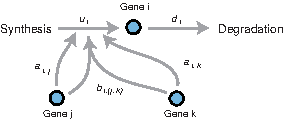end{document} is an active set of genes regulating the ith gene, and Δt is a minute displacement. Here, we set Δt = 1 (:a minimum observational interval) for simplicity. Figure 1 exemplifies this model.

FIG. 1.

An example of the combinatorial transcription model regarding the ith gene. A gene undergoes synthesis and degradation processes, and its synthesis process is regulated through individual effects a_i_,j,a_i_,k, and a combinatorial effect b_i_,(j,k).

In order to assimilate a simulation model and observational data, we apply a nonlinear state space model (Asif and Sanguinetti, 2011; Hirose et al., 2008; Kojima et al., 2010; Lillacci and Khammash, 2010; Quach et al., 2007). Let \documentclass{aastex}\usepackage{amsbsy}\usepackage{amsfonts}\usepackage{amssymb}\usepackage{bm}\usepackage{mathrsfs}\usepackage{pifont}\usepackage{stmaryrd}\usepackage{textcomp}\usepackage{portland, xspace}\usepackage{amsmath, amsxtra}\pagestyle{empty}\DeclareMathSizes{10}{9}{7}{6}\begin{document} $$\textbf{\textit{x}}_{t} = (x_{1 , t} , \ldots , x_{p , t}) ^{\prime}$$ \end{document} be the vector of hidden variables and y _t be the observational data at time t. A state space representation of Equation (2) is given by \documentclass{aastex}\usepackage{amsbsy}\usepackage{amsfonts}\usepackage{amssymb}\usepackage{bm}\usepackage{mathrsfs}\usepackage{pifont}\usepackage{stmaryrd}\usepackage{textcomp}\usepackage{portland, xspace}\usepackage{amsmath, amsxtra}\pagestyle{empty}\DeclareMathSizes{10}{9}{7}{6}\begin{document} \begin{align*}\textbf{\textit{x}}_{t + 1} = A\textbf{\textit{x}}_{t} + B {\rm vec} (\textbf{\textit{x}}_{t} \textbf{\textit{x}}_{t}^{\prime}) + \textbf{\textit{u}} + \textbf{\textit{v}}_{t} , \tag{3}\end{align*} \end{document} \documentclass{aastex}\usepackage{amsbsy}\usepackage{amsfonts}\usepackage{amssymb}\usepackage{bm}\usepackage{mathrsfs}\usepackage{pifont}\usepackage{stmaryrd}\usepackage{textcomp}\usepackage{portland, xspace}\usepackage{amsmath, amsxtra}\pagestyle{empty}\DeclareMathSizes{10}{9}{7}{6}\begin{document} \begin{align*}\textbf{\textit{y}}_{t} = \textbf{\textit{x}}_{t} + \textbf{\textit{w}}_{t} , \tag{4}\end{align*} \end{document}

where \documentclass{aastex}\usepackage{amsbsy}\usepackage{amsfonts}\usepackage{amssymb}\usepackage{bm}\usepackage{mathrsfs}\usepackage{pifont}\usepackage{stmaryrd}\usepackage{textcomp}\usepackage{portland, xspace}\usepackage{amsmath, amsxtra}\pagestyle{empty}\DeclareMathSizes{10}{9}{7}{6}\begin{document} $$A \in R^{p \times p}$$ \end{document} is a linear effect matrix, \documentclass{aastex}\usepackage{amsbsy}\usepackage{amsfonts}\usepackage{amssymb}\usepackage{bm}\usepackage{mathrsfs}\usepackage{pifont}\usepackage{stmaryrd}\usepackage{textcomp}\usepackage{portland, xspace}\usepackage{amsmath, amsxtra}\pagestyle{empty}\DeclareMathSizes{10}{9}{7}{6}\begin{document} $$B \in R^{p \times p^2}$$ \end{document} is a combinatorial effect matrix, vec(·) is a transformation function \documentclass{aastex}\usepackage{amsbsy}\usepackage{amsfonts}\usepackage{amssymb}\usepackage{bm}\usepackage{mathrsfs}\usepackage{pifont}\usepackage{stmaryrd}\usepackage{textcomp}\usepackage{portland, xspace}\usepackage{amsmath, amsxtra}\pagestyle{empty}\DeclareMathSizes{10}{9}{7}{6}\begin{document} $$(R^{p \times p} \rightarrow R^{p^2})$$ \end{document} , \documentclass{aastex}\usepackage{amsbsy}\usepackage{amsfonts}\usepackage{amssymb}\usepackage{bm}\usepackage{mathrsfs}\usepackage{pifont}\usepackage{stmaryrd}\usepackage{textcomp}\usepackage{portland, xspace}\usepackage{amsmath, amsxtra}\pagestyle{empty}\DeclareMathSizes{10}{9}{7}{6}\begin{document} $$\textbf{\textit{u}} = (u_{1} , \ldots , u_{p}) ^{\prime}$$ \end{document} , v _t ∼ N(0, Q), and w _t ∼ N(0, R) are system noise and observational noise with diagonal covariance matrices, respectively. Note that A and B should be sparse matrices according to \documentclass{aastex}\usepackage{amsbsy}\usepackage{amsfonts}\usepackage{amssymb}\usepackage{bm}\usepackage{mathrsfs}\usepackage{pifont}\usepackage{stmaryrd}\usepackage{textcomp}\usepackage{portland, xspace}\usepackage{amsmath, amsxtra}\pagestyle{empty}\DeclareMathSizes{10}{9}{7}{6}\begin{document} $${\cal A}_i$$ \end{document} , and that d _i is included in A. We define an entire set of time points \documentclass{aastex}\usepackage{amsbsy}\usepackage{amsfonts}\usepackage{amssymb}\usepackage{bm}\usepackage{mathrsfs}\usepackage{pifont}\usepackage{stmaryrd}\usepackage{textcomp}\usepackage{portland, xspace}\usepackage{amsmath, amsxtra}\pagestyle{empty}\DeclareMathSizes{10}{9}{7}{6}\begin{document} $${\cal T} = \{1 , \ldots , T \} $$ \end{document} and the observed time set \documentclass{aastex}\usepackage{amsbsy}\usepackage{amsfonts}\usepackage{amssymb}\usepackage{bm}\usepackage{mathrsfs}\usepackage{pifont}\usepackage{stmaryrd}\usepackage{textcomp}\usepackage{portland, xspace}\usepackage{amsmath, amsxtra}\pagestyle{empty}\DeclareMathSizes{10}{9}{7}{6}\begin{document} $${\cal T}_{obs} \ ({\cal T}_{obs} \subset {\cal T}).$$ \end{document}

2.2. Unscented Kalman filter

In Equations (3) and (4), conditional probability densities P( x _t|Y_t₋₁), P( x _t|Y_t), and P( x _t|Y_T) can be non-Gaussian forms, where \documentclass{aastex}\usepackage{amsbsy}\usepackage{amsfonts}\usepackage{amssymb}\usepackage{bm}\usepackage{mathrsfs}\usepackage{pifont}\usepackage{stmaryrd}\usepackage{textcomp}\usepackage{portland, xspace}\usepackage{amsmath, amsxtra}\pagestyle{empty}\DeclareMathSizes{10}{9}{7}{6}\begin{document} $$Y_{t} = (\textbf{\textit{y}}_{1} , \ldots , \textbf{\textit{y}}_{t})$$ \end{document} . Therefore, we applied the unscented Kalman filter (UKF) (Julier and Uhlmann, 1997, 2004; Chow et al., 2007) to approximately obtain these conditional probability densities. The procedure is explained below.

2.2.1. Prediction and filtering steps

Let x _t|s and V_t_|s be the expectation and the covariance matrix, given observational data Y_s at time t. For \documentclass{aastex}\usepackage{amsbsy}\usepackage{amsfonts}\usepackage{amssymb}\usepackage{bm}\usepackage{mathrsfs}\usepackage{pifont}\usepackage{stmaryrd}\usepackage{textcomp}\usepackage{portland, xspace}\usepackage{amsmath, amsxtra}\pagestyle{empty}\DeclareMathSizes{10}{9}{7}{6}\begin{document} $$t = 0 , \ldots , T - 1$$ \end{document} ,

1. Select sigma points \documentclass{aastex}\usepackage{amsbsy}\usepackage{amsfonts}\usepackage{amssymb}\usepackage{bm}\usepackage{mathrsfs}\usepackage{pifont}\usepackage{stmaryrd}\usepackage{textcomp}\usepackage{portland, xspace}\usepackage{amsmath, amsxtra}\pagestyle{empty}\DeclareMathSizes{10}{9}{7}{6}\begin{document} $$\textbf{\textit{x}}_{t \mid t}^{(n)} (n = 0 , \ldots , 2p)$$ \end{document} as \documentclass{aastex}\usepackage{amsbsy}\usepackage{amsfonts}\usepackage{amssymb}\usepackage{bm}\usepackage{mathrsfs}\usepackage{pifont}\usepackage{stmaryrd}\usepackage{textcomp}\usepackage{portland, xspace}\usepackage{amsmath, amsxtra}\pagestyle{empty}\DeclareMathSizes{10}{9}{7}{6}\begin{document} \begin{align*}\textbf{\textit{x}}_{t \mid t}^{(n)} = \textbf{\textit{x}}_{t \mid t} , \qquad \qquad \qquad \qquad (n = 0) , \tag{5}\end{align*} \end{document} \documentclass{aastex}\usepackage{amsbsy}\usepackage{amsfonts}\usepackage{amssymb}\usepackage{bm}\usepackage{mathrsfs}\usepackage{pifont}\usepackage{stmaryrd}\usepackage{textcomp}\usepackage{portland, xspace}\usepackage{amsmath, amsxtra}\pagestyle{empty}\DeclareMathSizes{10}{9}{7}{6}\begin{document} \begin{align*}\textbf{\textit{x}}_{t \mid t}^{(n)} = \textbf{\textit{x}}_{t \mid t} + \sqrt{(p + \lambda) \Sigma_{t \mid t}^{(n)}} , \qquad \qquad (n = 1 , \ldots , p) , \tag{6}\end{align*} \end{document} \documentclass{aastex}\usepackage{amsbsy}\usepackage{amsfonts}\usepackage{amssymb}\usepackage{bm}\usepackage{mathrsfs}\usepackage{pifont}\usepackage{stmaryrd}\usepackage{textcomp}\usepackage{portland, xspace}\usepackage{amsmath, amsxtra}\pagestyle{empty}\DeclareMathSizes{10}{9}{7}{6}\begin{document} \begin{align*}\textbf{\textit{x}}_{t \mid t}^{(n)} = \textbf{\textit{x}}_{t \mid t} - \sqrt{(p + \lambda) \Sigma_{t \mid t}^{(n - p)}} , \qquad \qquad (n = p + 1 , \ldots , 2p) , \tag{7}\end{align*} \end{document}

2. Predict the next state of the generated sigma points \documentclass{aastex}\usepackage{amsbsy}\usepackage{amsfonts}\usepackage{amssymb}\usepackage{bm}\usepackage{mathrsfs}\usepackage{pifont}\usepackage{stmaryrd}\usepackage{textcomp}\usepackage{portland, xspace}\usepackage{amsmath, amsxtra}\pagestyle{empty}\DeclareMathSizes{10}{9}{7}{6}\begin{document} $$\textbf{\textit{x}}_{t \mid t}^{(n)}$$ \end{document} as \documentclass{aastex}\usepackage{amsbsy}\usepackage{amsfonts}\usepackage{amssymb}\usepackage{bm}\usepackage{mathrsfs}\usepackage{pifont}\usepackage{stmaryrd}\usepackage{textcomp}\usepackage{portland, xspace}\usepackage{amsmath, amsxtra}\pagestyle{empty}\DeclareMathSizes{10}{9}{7}{6}\begin{document} $$\textbf{\textit{x}}_{t + 1 \mid t}^{(n)}$$ \end{document} using the system equation of Equation (3) without adding the system noise.

3. Calculate x _t+1|t and V_t_+1|t as \documentclass{aastex}\usepackage{amsbsy}\usepackage{amsfonts}\usepackage{amssymb}\usepackage{bm}\usepackage{mathrsfs}\usepackage{pifont}\usepackage{stmaryrd}\usepackage{textcomp}\usepackage{portland, xspace}\usepackage{amsmath, amsxtra}\pagestyle{empty}\DeclareMathSizes{10}{9}{7}{6}\begin{document} \begin{align*}\textbf{\textit{x}}_{t + 1 \mid t} = \sum_{n = 0}^{2p} {\cal W}^{(n)}_{1} \textbf{\textit{x}}_{t + 1 \mid t}^{(n)} , \tag{8}\end{align*} \end{document} \documentclass{aastex}\usepackage{amsbsy}\usepackage{amsfonts}\usepackage{amssymb}\usepackage{bm}\usepackage{mathrsfs}\usepackage{pifont}\usepackage{stmaryrd}\usepackage{textcomp}\usepackage{portland, xspace}\usepackage{amsmath, amsxtra}\pagestyle{empty}\DeclareMathSizes{10}{9}{7}{6}\begin{document} \begin{align*}\Sigma_{t + 1 \mid t} = \sum_{n = 0}^{2p} {\cal W}^{(n)}_{2} (\textbf{\textit{x}}_{t + 1 \mid t}^{(n)} - \textbf{\textit{x}}_{t + 1 \mid t}) (\textbf{\textit{x}}_{t + 1 \mid t}^{(n)} - \textbf{\textit{x}}_{t + 1 \mid t}) ^{\prime} + Q , \tag{9}\end{align*} \end{document} \documentclass{aastex}\usepackage{amsbsy}\usepackage{amsfonts}\usepackage{amssymb}\usepackage{bm}\usepackage{mathrsfs}\usepackage{pifont}\usepackage{stmaryrd}\usepackage{textcomp}\usepackage{portland, xspace}\usepackage{amsmath, amsxtra}\pagestyle{empty}\DeclareMathSizes{10}{9}{7}{6}\begin{document} \begin{align*} {\cal W} ^ {(0)} _ {1} = \frac {\lambda} {p + \lambda} , \tag {10} \end{align*} \end{document} \documentclass{aastex}\usepackage{amsbsy}\usepackage{amsfonts}\usepackage{amssymb}\usepackage{bm}\usepackage{mathrsfs}\usepackage{pifont}\usepackage{stmaryrd}\usepackage{textcomp}\usepackage{portland, xspace}\usepackage{amsmath, amsxtra}\pagestyle{empty}\DeclareMathSizes{10}{9}{7}{6}\begin{document} \begin{align*} {\cal W} ^ {(0)} _ {2} = \frac {\lambda} {p + \lambda} + 1 - \alpha^ {2} + \beta , \tag {11} \end{align*} \end{document} \documentclass{aastex}\usepackage{amsbsy}\usepackage{amsfonts}\usepackage{amssymb}\usepackage{bm}\usepackage{mathrsfs}\usepackage{pifont}\usepackage{stmaryrd}\usepackage{textcomp}\usepackage{portland, xspace}\usepackage{amsmath, amsxtra}\pagestyle{empty}\DeclareMathSizes{10}{9}{7}{6}\begin{document} \begin{align*} {\cal W} ^ {(n)} _ {1} = {\cal W} ^ {(n)} _ {2} = \frac {1} {2 (p + \lambda)} , \ (n = 1 , \ldots , 2p) , \tag {12} \end{align*} \end{document}

where β is set 2 (Julier, 2002).

4. In the combinatorial model, the observational equation of Equation (4) is a linear function. Then, we can apply the general Kalman filter algorithm (Kojima et al., 2010; Kalman, 1960) to obtain the optimal conditional expectation and covariance matrix as follows \documentclass{aastex}\usepackage{amsbsy}\usepackage{amsfonts}\usepackage{amssymb}\usepackage{bm}\usepackage{mathrsfs}\usepackage{pifont}\usepackage{stmaryrd}\usepackage{textcomp}\usepackage{portland, xspace}\usepackage{amsmath, amsxtra}\pagestyle{empty}\DeclareMathSizes{10}{9}{7}{6}\begin{document} \begin{align*}\textbf{\textit{x}}_{t + 1 \mid t + 1} = \textbf{\textit{x}}_{t + 1 \mid t} + \Sigma_{t + 1 \mid t + 1} R^{- 1} (\textbf{\textit{y}}_{t + 1} - \textbf{\textit{x}}_{t + 1 \mid t}) , \tag{13}\end{align*} \end{document} \documentclass{aastex}\usepackage{amsbsy}\usepackage{amsfonts}\usepackage{amssymb}\usepackage{bm}\usepackage{mathrsfs}\usepackage{pifont}\usepackage{stmaryrd}\usepackage{textcomp}\usepackage{portland, xspace}\usepackage{amsmath, amsxtra}\pagestyle{empty}\DeclareMathSizes{10}{9}{7}{6}\begin{document} \begin{align*}\Sigma_{t + 1 \mid t + 1} = (R^{- 1} + \Sigma_{t + 1 \mid t}^{- 1}) ^{- 1}. \tag{14}\end{align*} \end{document}

More details can be referred to in Julier and Uhlmann (1997, 2004).

2.2.2. Smoothing step

In order to obtain the conditional expectation and covariance matrix of the hidden state given full observational data Y _T, we apply the Rauch-Tung-Striebel (RTS) smoother for UKF (Sarkka, 2008). The formulation of the RTS smoother is described as follows: \documentclass{aastex}\usepackage{amsbsy}\usepackage{amsfonts}\usepackage{amssymb}\usepackage{bm}\usepackage{mathrsfs}\usepackage{pifont}\usepackage{stmaryrd}\usepackage{textcomp}\usepackage{portland, xspace}\usepackage{amsmath, amsxtra}\pagestyle{empty}\DeclareMathSizes{10}{9}{7}{6}\begin{document} \begin{align*}\textbf{\textit{x}}_{t \mid T} = \textbf{\textit{x}}_{t \mid t} + K_{t} (\textbf{\textit{x}}_{t + 1 \mid T} - \textbf{\textit{x}}_{t + 1 \mid t - 1}) , \tag{15}\end{align*} \end{document} \documentclass{aastex}\usepackage{amsbsy}\usepackage{amsfonts}\usepackage{amssymb}\usepackage{bm}\usepackage{mathrsfs}\usepackage{pifont}\usepackage{stmaryrd}\usepackage{textcomp}\usepackage{portland, xspace}\usepackage{amsmath, amsxtra}\pagestyle{empty}\DeclareMathSizes{10}{9}{7}{6}\begin{document} \begin{align*}\Sigma_{t \mid T} = \Sigma_{t \mid t} + K_{t} (\Sigma_{t + 1 \mid T} - \Sigma_{t + 1 \mid t - 1}) K_{t}^{\prime} , \tag{16}\end{align*} \end{document} \documentclass{aastex}\usepackage{amsbsy}\usepackage{amsfonts}\usepackage{amssymb}\usepackage{bm}\usepackage{mathrsfs}\usepackage{pifont}\usepackage{stmaryrd}\usepackage{textcomp}\usepackage{portland, xspace}\usepackage{amsmath, amsxtra}\pagestyle{empty}\DeclareMathSizes{10}{9}{7}{6}\begin{document} \begin{align*}K_{t} = C_{t} \Sigma_{t + 1 \mid t}^{- 1} , \tag{17}\end{align*} \end{document} \documentclass{aastex}\usepackage{amsbsy}\usepackage{amsfonts}\usepackage{amssymb}\usepackage{bm}\usepackage{mathrsfs}\usepackage{pifont}\usepackage{stmaryrd}\usepackage{textcomp}\usepackage{portland, xspace}\usepackage{amsmath, amsxtra}\pagestyle{empty}\DeclareMathSizes{10}{9}{7}{6}\begin{document} \begin{align*}C_{t} = \sum_{n = 0}^{2p} {\cal W}^{(n)}_{2} (\textbf{\textit{x}}_{t \mid t - 1}^{(n)} - \textbf{\textit{x}}_{t \mid t - 1}) (\textbf{\textit{x}}_{t + 1 \mid t}^{(n)} - \textbf{\textit{x}}_{t + 1 \mid t}) ^{\prime}. \tag{18}\end{align*} \end{document}

Since we have x _T|T and Σ_T|T after prediction and filtering steps, the above equations are recursively applied for \documentclass{aastex}\usepackage{amsbsy}\usepackage{amsfonts}\usepackage{amssymb}\usepackage{bm}\usepackage{mathrsfs}\usepackage{pifont}\usepackage{stmaryrd}\usepackage{textcomp}\usepackage{portland, xspace}\usepackage{amsmath, amsxtra}\pagestyle{empty}\DeclareMathSizes{10}{9}{7}{6}\begin{document} $$t = T - 1 , \ldots , 0$$ \end{document} .

2.3. Parameter estimation using EM-algorithm

Let \documentclass{aastex}\usepackage{amsbsy}\usepackage{amsfonts}\usepackage{amssymb}\usepackage{bm}\usepackage{mathrsfs}\usepackage{pifont}\usepackage{stmaryrd}\usepackage{textcomp}\usepackage{portland, xspace}\usepackage{amsmath, amsxtra}\pagestyle{empty}\DeclareMathSizes{10}{9}{7}{6}\begin{document} $$X_T = \{\textbf{\textit{x}}_0 , \ldots , \textbf{\textit{x}}_T \} $$ \end{document} be the set of state variables, and θ = {A, B, u , Q, R, μ ₀} be the parameter vector. The log-likelihood of observational data is given by \documentclass{aastex}\usepackage{amsbsy}\usepackage{amsfonts}\usepackage{amssymb}\usepackage{bm}\usepackage{mathrsfs}\usepackage{pifont}\usepackage{stmaryrd}\usepackage{textcomp}\usepackage{portland, xspace}\usepackage{amsmath, amsxtra}\pagestyle{empty}\DeclareMathSizes{10}{9}{7}{6}\begin{document} \begin{align*}\log L = \log \int P (\textbf{\textit{x}}_{0}) \prod_{t \in {\cal T}} P (\textbf{\textit{x}}_{t} \mid \textbf{\textit{x}}_{t - 1}) \prod_{t \in {\cal T}_{obs}}P (\textbf{\textit{y}}_{t} \mid \textbf{\textit{x}}_{t}) d\textbf{\textit{x}}_{1} \ldots d\textbf{\textit{x}}_{T} , \tag{19}\end{align*} \end{document}

where P( x ₀) is a probability density of N-dimensional Gaussian distributions N( μ ₀, Σ₀), P( x _t| x _t−1) and P( y _t| x _t) can be probability densities of N-dimensional non-Gaussian distributions approximated by Equations (3) and (4) in section 2.1 and the unscented transformation in section 2.2.

In this article, we attempted to estimate the parameter vector θ by maximizing Equation (19) using the EM-algorithm (Dempster et al., 1977). Thus, the conditional expectation of the joint log-likelihood of the complete data (X_T,Y_T) at the lth iteration, \documentclass{aastex}\usepackage{amsbsy}\usepackage{amsfonts}\usepackage{amssymb}\usepackage{bm}\usepackage{mathrsfs}\usepackage{pifont}\usepackage{stmaryrd}\usepackage{textcomp}\usepackage{portland, xspace}\usepackage{amsmath, amsxtra}\pagestyle{empty}\DeclareMathSizes{10}{9}{7}{6}\begin{document} \begin{align*}q ({\bold \theta} \mid {\bold \theta}_{l}) = E [ \log P (Y_{T} , X_{T} \mid {\bold \theta}) \mid Y_{T} , {\bold \theta}_{l} ] , \tag{20}\end{align*} \end{document}

is iteratively maximized with respect to θ until convergence.

In the expectation step, set conditional expectations of x _t as \documentclass{aastex}\usepackage{amsbsy}\usepackage{amsfonts}\usepackage{amssymb}\usepackage{bm}\usepackage{mathrsfs}\usepackage{pifont}\usepackage{stmaryrd}\usepackage{textcomp}\usepackage{portland, xspace}\usepackage{amsmath, amsxtra}\pagestyle{empty}\DeclareMathSizes{10}{9}{7}{6}\begin{document} \begin{align*}V_{t} = \sum_{t \in {\cal T}} \sum^{2p}_{n = 0}{\cal W}_{2}^{(n)} \textbf{\textit{x}}^{(n)}_{t \mid T}\textbf{\textit{x}}^{(n) ^{\prime}}_{t \mid T} , \tag{21}\end{align*} \end{document} \documentclass{aastex}\usepackage{amsbsy}\usepackage{amsfonts}\usepackage{amssymb}\usepackage{bm}\usepackage{mathrsfs}\usepackage{pifont}\usepackage{stmaryrd}\usepackage{textcomp}\usepackage{portland, xspace}\usepackage{amsmath, amsxtra}\pagestyle{empty}\DeclareMathSizes{10}{9}{7}{6}\begin{document} \begin{align*}V_{lag} = \sum_{t \in {\cal T}} \sum^{2p}_{n = 0}{\cal W}_{2}^{(n)} \textbf{\textit{x}}^{(n)}_{t \mid T}\textbf{\textit{x}}^{(n) ^{\prime}}_{t - 1 \mid T} , \tag{22}\end{align*} \end{document} \documentclass{aastex}\usepackage{amsbsy}\usepackage{amsfonts}\usepackage{amssymb}\usepackage{bm}\usepackage{mathrsfs}\usepackage{pifont}\usepackage{stmaryrd}\usepackage{textcomp}\usepackage{portland, xspace}\usepackage{amsmath, amsxtra}\pagestyle{empty}\DeclareMathSizes{10}{9}{7}{6}\begin{document} \begin{align*}V_{t - 1} = \sum_{t \in {\cal T}} \sum^{2p}_{n = 0}{\cal W}_{2}^{(n)} \textbf{\textit{x}}^{(n)}_{t - 1 \mid T}\textbf{\textit{x}}^{(n) ^{\prime}}_{t - 1 \mid T} , \tag{23}\end{align*} \end{document} \documentclass{aastex}\usepackage{amsbsy}\usepackage{amsfonts}\usepackage{amssymb}\usepackage{bm}\usepackage{mathrsfs}\usepackage{pifont}\usepackage{stmaryrd}\usepackage{textcomp}\usepackage{portland, xspace}\usepackage{amsmath, amsxtra}\pagestyle{empty}\DeclareMathSizes{10}{9}{7}{6}\begin{document} \begin{align*}\Phi_{lag} = \sum_{t \in {\cal T}} \sum^{2p}_{n = 0}{\cal W}_{2}^{(n)}\textbf{\textit{x}}^{(n)}_{t \mid T} {\rm vec} (\textbf{\textit{x}}^{(n)}_{t - 1 \mid T} \textbf{\textit{x}}^{(n) ^{\prime}}_{t - 1 \mid T}) ^{\prime} , \tag{24}\end{align*} \end{document} \documentclass{aastex}\usepackage{amsbsy}\usepackage{amsfonts}\usepackage{amssymb}\usepackage{bm}\usepackage{mathrsfs}\usepackage{pifont}\usepackage{stmaryrd}\usepackage{textcomp}\usepackage{portland, xspace}\usepackage{amsmath, amsxtra}\pagestyle{empty}\DeclareMathSizes{10}{9}{7}{6}\begin{document} \begin{align*}\Phi_{t - 1} = \sum_{t \in {\cal T}} \sum^{2p}_{n = 0}{\cal W}_{2}^{(n)}\textbf{\textit{x}}^{(n)}_{t - 1 \mid T} {\rm vec} (\textbf{\textit{x}}^{(n)}_{t - 1 \mid T} \textbf{\textit{x}}^{(n) ^{\prime}}_{t - 1 \mid T}) ^{\prime} , \tag{25}\end{align*} \end{document} \documentclass{aastex}\usepackage{amsbsy}\usepackage{amsfonts}\usepackage{amssymb}\usepackage{bm}\usepackage{mathrsfs}\usepackage{pifont}\usepackage{stmaryrd}\usepackage{textcomp}\usepackage{portland, xspace}\usepackage{amsmath, amsxtra}\pagestyle{empty}\DeclareMathSizes{10}{9}{7}{6}\begin{document} \begin{align*}\Psi_{t - 1} = \sum_{t \in {\cal T}} \sum^{2p}_{n = 0}{\cal W}_{2}^{(n)}{\rm vec} (\textbf{\textit{x}}^{(n)}_{t - 1 \mid T} \textbf{\textit{x}}^{(n) ^{\prime}}_{t - 1 \mid T}) {\rm vec} (\textbf{\textit{x}}^{(n)}_{t - 1 \mid T} \textbf{\textit{x}}^{(n) ^{\prime}}_{t - 1 \mid T}) ^{\prime}, \tag{26}\end{align*} \end{document} \documentclass{aastex}\usepackage{amsbsy}\usepackage{amsfonts}\usepackage{amssymb}\usepackage{bm}\usepackage{mathrsfs}\usepackage{pifont}\usepackage{stmaryrd}\usepackage{textcomp}\usepackage{portland, xspace}\usepackage{amsmath, amsxtra}\pagestyle{empty}\DeclareMathSizes{10}{9}{7}{6}\begin{document} \begin{align*}\textbf{\textit{s}}_{t} = \sum_{t \in {\cal T}} \sum^{2p}_{n = 0}{\cal W}_{1}^{(n)}\textbf{\textit{x}}^{(n)}_{t \mid T} , \tag{27}\end{align*} \end{document} \documentclass{aastex}\usepackage{amsbsy}\usepackage{amsfonts}\usepackage{amssymb}\usepackage{bm}\usepackage{mathrsfs}\usepackage{pifont}\usepackage{stmaryrd}\usepackage{textcomp}\usepackage{portland, xspace}\usepackage{amsmath, amsxtra}\pagestyle{empty}\DeclareMathSizes{10}{9}{7}{6}\begin{document} \begin{align*}\textbf{\textit{s}}_{t - 1} = \sum_{t \in {\cal T}} \sum^{2p}_{n = 0}{\cal W}_{1}^{(n)}\textbf{\textit{x}}^{(n)}_{t - 1 \mid T} , \tag{28}\end{align*} \end{document} \documentclass{aastex}\usepackage{amsbsy}\usepackage{amsfonts}\usepackage{amssymb}\usepackage{bm}\usepackage{mathrsfs}\usepackage{pifont}\usepackage{stmaryrd}\usepackage{textcomp}\usepackage{portland, xspace}\usepackage{amsmath, amsxtra}\pagestyle{empty}\DeclareMathSizes{10}{9}{7}{6}\begin{document} \begin{align*}\textbf{\textit{s}}^{2}_{t - 1} = \sum_{t \in {\cal T}} \sum^{2p}_{n = 0}{\cal W}_{1}^{(n)} {\rm vec} (\textbf{\textit{x}}^{(n)}_{t - 1 \mid T} \textbf{\textit{x}}^{(n) ^{\prime}}_{t - 1 \mid T}) ^{\prime}. \tag{29}\end{align*} \end{document}

In the maximization step, θ _l is updated to θ _l+1 = arg max_θq( θ | θ _l). Let v _lag,i, φ _lag,i, and φ _t-1,i be a transpose of the ith row vector of V_lag, Ф_lag, and Ф_t−1, respectively. Then, θ is updated as \documentclass{aastex}\usepackage{amsbsy}\usepackage{amsfonts}\usepackage{amssymb}\usepackage{bm}\usepackage{mathrsfs}\usepackage{pifont}\usepackage{stmaryrd}\usepackage{textcomp}\usepackage{portland, xspace}\usepackage{amsmath, amsxtra}\pagestyle{empty}\DeclareMathSizes{10}{9}{7}{6}\begin{document} \begin{align*}\textbf{\textit{a}}_{i}^{\cal A} = V_{t - 1}^{{\cal A}^{- 1}} (\textbf{\textit{v}}_{lag , i}^{\cal A} - \phi_{t - 1}^{{\cal A} \times {\cal B}}\textbf{\textit{b}}_{i}^{\cal B} - u_{i}\textbf{\textit{s}}_{t - 1}^{\cal A}) , \tag{30}\end{align*} \end{document} \documentclass{aastex}\usepackage{amsbsy}\usepackage{amsfonts}\usepackage{amssymb}\usepackage{bm}\usepackage{mathrsfs}\usepackage{pifont}\usepackage{stmaryrd}\usepackage{textcomp}\usepackage{portland, xspace}\usepackage{amsmath, amsxtra}\pagestyle{empty}\DeclareMathSizes{10}{9}{7}{6}\begin{document} \begin{align*}\textbf{\textit{b}}_{i}^{\cal B} = \Psi_{t - 1}^{{\cal B}^{- 1}} (\phi_{lag , i}^{\cal B} - \phi_{t - 1}^{{\cal A} \times {\cal B}^{\prime}} \textbf{\textit{a}}_{i}^{\cal A} - u_{i}\textbf{\textit{s}}^{2^{\cal B}}) , \tag{31}\end{align*} \end{document} \documentclass{aastex}\usepackage{amsbsy}\usepackage{amsfonts}\usepackage{amssymb}\usepackage{bm}\usepackage{mathrsfs}\usepackage{pifont}\usepackage{stmaryrd}\usepackage{textcomp}\usepackage{portland, xspace}\usepackage{amsmath, amsxtra}\pagestyle{empty}\DeclareMathSizes{10}{9}{7}{6}\begin{document} \begin{align*}\textbf {\textit {u}} = \frac {\textbf {\textit {s}} _ {t} - A\textbf {\textit {s}} _ {t - 1} - B\textbf {\textit {s}} ^2} {T} , \tag {32} \end{align*} \end{document} \documentclass{aastex}\usepackage{amsbsy}\usepackage{amsfonts}\usepackage{amssymb}\usepackage{bm}\usepackage{mathrsfs}\usepackage{pifont}\usepackage{stmaryrd}\usepackage{textcomp}\usepackage{portland, xspace}\usepackage{amsmath, amsxtra}\pagestyle{empty}\DeclareMathSizes{10}{9}{7}{6}\begin{document} \begin{align*} Q & = \frac {1} {T} \sum^ {T} _ {t = 1} E [ (\textbf {\textit {x}} _ {t} - A\textbf {\textit {x}} _ {t - 1} - B {\rm vec} (\textbf {\textit {x}} _ {t - 1} \textbf {\textit {x}} _ {t - 1} ^ {\prime}) - \textbf {\textit {u}}) \cdot (\textbf {\textit {x}} _ {t} - A\textbf {\textit {x}} _ {t - 1} - B {\rm vec} (\textbf {\textit {x}} _ {t - 1} \textbf {\textit {x}} _ {t - 1} ^ {\prime}) - \textbf {\textit {u}} ^ {\prime} \mid Y_ {T} ] , & (33) \end{align*} \end{document} \documentclass{aastex}\usepackage{amsbsy}\usepackage{amsfonts}\usepackage{amssymb}\usepackage{bm}\usepackage{mathrsfs}\usepackage{pifont}\usepackage{stmaryrd}\usepackage{textcomp}\usepackage{portland, xspace}\usepackage{amsmath, amsxtra}\pagestyle{empty}\DeclareMathSizes{10}{9}{7}{6}\begin{document} \begin{align*}{\bold \mu}_{0} = \textbf{\textit{x}}_{0 \mid T} , \tag{34}\end{align*} \end{document} \documentclass{aastex}\usepackage{amsbsy}\usepackage{amsfonts}\usepackage{amssymb}\usepackage{bm}\usepackage{mathrsfs}\usepackage{pifont}\usepackage{stmaryrd}\usepackage{textcomp}\usepackage{portland, xspace}\usepackage{amsmath, amsxtra}\pagestyle{empty}\DeclareMathSizes{10}{9}{7}{6}\begin{document} \begin{align*}R = \frac {1} {T} \sum_ {t \in {\cal T} _ {obs}} \{(\textbf {\textit {y}} _ {t} - \textbf {\textit {x}} _ {t \mid T}) (\textbf {\textit {y}} _ {t} - \textbf {\textit {x}} _ {t \mid T}) ^ {\prime} + \Sigma_ {t \mid T} \} , \tag {35} \end{align*} \end{document}

2.4. Network restoration algorithm

When an original gene regulatory network \documentclass{aastex}\usepackage{amsbsy}\usepackage{amsfonts}\usepackage{amssymb}\usepackage{bm}\usepackage{mathrsfs}\usepackage{pifont}\usepackage{stmaryrd}\usepackage{textcomp}\usepackage{portland, xspace}\usepackage{amsmath, amsxtra}\pagestyle{empty}\DeclareMathSizes{10}{9}{7}{6}\begin{document} $${\cal M}_{original}$$ \end{document} is given, the purpose is to find the model \documentclass{aastex}\usepackage{amsbsy}\usepackage{amsfonts}\usepackage{amssymb}\usepackage{bm}\usepackage{mathrsfs}\usepackage{pifont}\usepackage{stmaryrd}\usepackage{textcomp}\usepackage{portland, xspace}\usepackage{amsmath, amsxtra}\pagestyle{empty}\DeclareMathSizes{10}{9}{7}{6}\begin{document} $${\cal M}_{best}$$ \end{document} that can best predict observational data. Here, the prediction ability of a model \documentclass{aastex}\usepackage{amsbsy}\usepackage{amsfonts}\usepackage{amssymb}\usepackage{bm}\usepackage{mathrsfs}\usepackage{pifont}\usepackage{stmaryrd}\usepackage{textcomp}\usepackage{portland, xspace}\usepackage{amsmath, amsxtra}\pagestyle{empty}\DeclareMathSizes{10}{9}{7}{6}\begin{document} $${\cal M}$$ \end{document} is evaluated using the Bayesian information criterion (BIC) (Schwarz, 1978) described by \documentclass{aastex}\usepackage{amsbsy}\usepackage{amsfonts}\usepackage{amssymb}\usepackage{bm}\usepackage{mathrsfs}\usepackage{pifont}\usepackage{stmaryrd}\usepackage{textcomp}\usepackage{portland, xspace}\usepackage{amsmath, amsxtra}\pagestyle{empty}\DeclareMathSizes{10}{9}{7}{6}\begin{document} \begin{align*}BIC = 2 \log L - D \log \nu , \tag{36}\end{align*} \end{document}

where D and ν are the number of samples and the nonzero parameters, respectively. Because of the high computational cost involved in estimating the values of the parameters θ for \documentclass{aastex}\usepackage{amsbsy}\usepackage{amsfonts}\usepackage{amssymb}\usepackage{bm}\usepackage{mathrsfs}\usepackage{pifont}\usepackage{stmaryrd}\usepackage{textcomp}\usepackage{portland, xspace}\usepackage{amsmath, amsxtra}\pagestyle{empty}\DeclareMathSizes{10}{9}{7}{6}\begin{document} $${\cal M}$$ \end{document} , we can not evaluate all candidate models. Therefore, starting from \documentclass{aastex}\usepackage{amsbsy}\usepackage{amsfonts}\usepackage{amssymb}\usepackage{bm}\usepackage{mathrsfs}\usepackage{pifont}\usepackage{stmaryrd}\usepackage{textcomp}\usepackage{portland, xspace}\usepackage{amsmath, amsxtra}\pagestyle{empty}\DeclareMathSizes{10}{9}{7}{6}\begin{document} $${\cal M}_{original}$$ \end{document} , one strategy is to sequentially evaluate candidate models that are constructed by changing a part of the regulatory structure of the current model \documentclass{aastex}\usepackage{amsbsy}\usepackage{amsfonts}\usepackage{amssymb}\usepackage{bm}\usepackage{mathrsfs}\usepackage{pifont}\usepackage{stmaryrd}\usepackage{textcomp}\usepackage{portland, xspace}\usepackage{amsmath, amsxtra}\pagestyle{empty}\DeclareMathSizes{10}{9}{7}{6}\begin{document} $${\cal M}_{current}$$ \end{document} of which prediction ability is the best among evaluated ones. In this paradigm, we consider three operations, that is, adding, deleting, and replacing a regulation, which are shown in Figure 2, and the constraints add_max and del_max, which restrict the number of additional and deleted regulations from \documentclass{aastex}\usepackage{amsbsy}\usepackage{amsfonts}\usepackage{amssymb}\usepackage{bm}\usepackage{mathrsfs}\usepackage{pifont}\usepackage{stmaryrd}\usepackage{textcomp}\usepackage{portland, xspace}\usepackage{amsmath, amsxtra}\pagestyle{empty}\DeclareMathSizes{10}{9}{7}{6}\begin{document} $${\cal M}_{original}$$ \end{document} . Then, we propose a novel algorithm, which can efficiently evaluate only highly possible candidates, for improving and extending GRNs to obtain \documentclass{aastex}\usepackage{amsbsy}\usepackage{amsfonts}\usepackage{amssymb}\usepackage{bm}\usepackage{mathrsfs}\usepackage{pifont}\usepackage{stmaryrd}\usepackage{textcomp}\usepackage{portland, xspace}\usepackage{amsmath, amsxtra}\pagestyle{empty}\DeclareMathSizes{10}{9}{7}{6}\begin{document} $${\cal M}_{best}$$ \end{document} as concluded in Algorithms 1 –3 (2 and 3 are sub-algorithms for Algorithm 1). In these algorithms, we consider a function for measuring the possibility of the model \documentclass{aastex}\usepackage{amsbsy}\usepackage{amsfonts}\usepackage{amssymb}\usepackage{bm}\usepackage{mathrsfs}\usepackage{pifont}\usepackage{stmaryrd}\usepackage{textcomp}\usepackage{portland, xspace}\usepackage{amsmath, amsxtra}\pagestyle{empty}\DeclareMathSizes{10}{9}{7}{6}\begin{document} $${\cal M}$$ \end{document} that added or deleted a regulation to the ith gene from \documentclass{aastex}\usepackage{amsbsy}\usepackage{amsfonts}\usepackage{amssymb}\usepackage{bm}\usepackage{mathrsfs}\usepackage{pifont}\usepackage{stmaryrd}\usepackage{textcomp}\usepackage{portland, xspace}\usepackage{amsmath, amsxtra}\pagestyle{empty}\DeclareMathSizes{10}{9}{7}{6}\begin{document} $${\cal M}_{current}$$ \end{document} as \documentclass{aastex}\usepackage{amsbsy}\usepackage{amsfonts}\usepackage{amssymb}\usepackage{bm}\usepackage{mathrsfs}\usepackage{pifont}\usepackage{stmaryrd}\usepackage{textcomp}\usepackage{portland, xspace}\usepackage{amsmath, amsxtra}\pagestyle{empty}\DeclareMathSizes{10}{9}{7}{6}\begin{document} \begin{align*}e ({\cal M} , i) = \textbf{\textit{a}}_{i}^{\prime} V_{t - 1} \textbf{\textit{a}}_{i} - 2 \textbf{\textit{v}}_{lag , i} \textbf{\textit{a}}_{i} + 2 \textbf{\textit{b}}_{i}^{\prime} \phi^{\prime}_{t - 1} \textbf{\textit{a}}_{i} + 2u_{i} \textbf{\textit{s}}^{\prime}_{t - 1} \textbf{\textit{a}}_{i}. \tag{37}\end{align*} \end{document}

FIG. 2.

The operations of changing the current network. We consider the three types of operations for an improvement of gene regulatory network (GRN), that is, “Add Edge” (adding), “Delete Edge” (deleting), and “Replace Edge” (replacing). Under the constraints of add_max and del_max, these operations are recursively executed until the network cannot be changed through these operations to decrease the Bayesian information criterion (BIC) score.

Algorithm 1. The proposed algorithm for improving GRNs based on the approximate posterior probability

1: Set r;

2: add ← 0; del ← 0; flag ← 0

3: BIC_current ← the BIC score of the original model;

\documentclass{aastex}\usepackage{amsbsy}\usepackage{amsfonts}\usepackage{amssymb}\usepackage{bm}\usepackage{mathrsfs}\usepackage{pifont}\usepackage{stmaryrd}\usepackage{textcomp}\usepackage{portland, xspace}\usepackage{amsmath, amsxtra}\pagestyle{empty}\DeclareMathSizes{10}{9}{7}{6}\begin{document} $${\cal M}_{current} \leftarrow {\cal M}_{original}$$ \end{document}

;

5: while flag < N² do

6: for i = 1 to N do

7: for j = 1 to N do

8: if A_i,j of

then

9: changed ← Execute subalgorithm 1;

10: else

11: changed ← Execute subalgorithm 2;

12: end if

13: if changed then

14: flag ← 0;

15: else

16: flag ← flag + 1;

17: end if

18: if flag >= N² then

19: break;

20: end if

21: end for

22: if flag >= N² then

23: break;

24: end if

25: end for

26: end while

Algorithm 2. Subalgorithm 1

1: changed ← FALSE;

2: Consider

that is constructed from

by setting a regulation to the ith gene by the jth gene as an active element;

3: Estimate the parameter values and obtain the BIC score BIC_candidate by the UKF and the EM-algorithm;

4: if BIC_current > BIC_candidate and add_max > add then

5: Set

; BIC_candidate ← BIC_current;

6: changed ← TRUE;

7: else

8: for i = 1 to N do

9: for k = 1 to r do

10: j ← the kth minimum element with respect to

\documentclass{aastex}\usepackage{amsbsy}\usepackage{amsfonts}\usepackage{amssymb}\usepackage{bm}\usepackage{mathrsfs}\usepackage{pifont}\usepackage{stmaryrd}\usepackage{textcomp}\usepackage{portland, xspace}\usepackage{amsmath, amsxtra}\pagestyle{empty}\DeclareMathSizes{10}{9}{7}{6}\begin{document} $$e (i , j_{col}) \ (j_{col} = 1 , \ldots , N)$$ \end{document}

;

11: if A_i,j of

is 0 then

12: continue;

13: end if

14: if A_i,j of

is 1 or add_max > add then

15: continue;

16: end if

17: Consider

that is constructed from

by setting a regulation to the ith gene by the jth gene as a nonactive set;

18: Estimate the parameter values and obtain the BIC score by the UKF and the EM-algorithm;

19: end for

20: end for

21: if BIC_current >the minimum BIC score among models calculated above then

22: Set

and BIC_current as those of the minimum one;

23: changed ← TRUE;

24: end if

25: end if

26: Set add and del as those of the

;

27: return changed;

Algorithm 3. Subalgorithm 2

1: changed ← FALSE;

2: Consider

that is constructed from

by setting a regulation to the ith gene by the jth gene as a non-active element;

3: Estimate the parameter values and obtain the BIC score BIC_candidate by the UKF and the EM-algorithm;

4: if BIC_current > BIC_candidate and del_max > del then

5: Set

; BIC_candidate ← BIC_current;

6: changed ← TRUE;

7: else

8: for i = 1 to N do

9: for k = 1 to r do

10: j ← the kth minimum element with respect to

\documentclass{aastex}\usepackage{amsbsy}\usepackage{amsfonts}\usepackage{amssymb}\usepackage{bm}\usepackage{mathrsfs}\usepackage{pifont}\usepackage{stmaryrd}\usepackage{textcomp}\usepackage{portland, xspace}\usepackage{amsmath, amsxtra}\pagestyle{empty}\DeclareMathSizes{10}{9}{7}{6}\begin{document} $$e (i , j_{col}) \ (j_{col} = 1 , \ldots , N)$$ \end{document}

;

11: if A_i_,j of

is 1 then

12: continue;

13: end if

14: if A_i_,j of

is 0 or add_del > del then

15: continue;

16: end if

17: Consider

that is constructed from

by setting a regulation to the ith gene by the jth gene as an active set;

18: Estimate the parameter values and obtain the BIC score by the UKF and the EM-algorithm;

19: end for

20: end for

21: if BIC_current >the minimum BIC score among models calculated above then

22: Set

and BIC_current as those of the minimum one;

23: changed ← TRUE;

24: end if

25: end if

26: Set add and del as those of the

;

27: return changed;

To measure the effectiveness of the candidate models when changing active sets, Equation (37), of which active sets are changed as those of the next candidate, is calculated. Then, only for r top models with respect to \documentclass{aastex}\usepackage{amsbsy}\usepackage{amsfonts}\usepackage{amssymb}\usepackage{bm}\usepackage{mathrsfs}\usepackage{pifont}\usepackage{stmaryrd}\usepackage{textcomp}\usepackage{portland, xspace}\usepackage{amsmath, amsxtra}\pagestyle{empty}\DeclareMathSizes{10}{9}{7}{6}\begin{document} $$- e ({\cal M} , i)$$ \end{document} for each i, the BIC scores are evaluated by estimating the parameter values maximizing prediction ability for observational data using UKF and the EM-algorithm. This procedure is shown in Figure 3. Note that \documentclass{aastex}\usepackage{amsbsy}\usepackage{amsfonts}\usepackage{amssymb}\usepackage{bm}\usepackage{mathrsfs}\usepackage{pifont}\usepackage{stmaryrd}\usepackage{textcomp}\usepackage{portland, xspace}\usepackage{amsmath, amsxtra}\pagestyle{empty}\DeclareMathSizes{10}{9}{7}{6}\begin{document} $$e ({\cal M} , i)$$ \end{document} can be derived when calculating arg arg \documentclass{aastex}\usepackage{amsbsy}\usepackage{amsfonts}\usepackage{amssymb}\usepackage{bm}\usepackage{mathrsfs}\usepackage{pifont}\usepackage{stmaryrd}\usepackage{textcomp}\usepackage{portland, xspace}\usepackage{amsmath, amsxtra}\pagestyle{empty}\DeclareMathSizes{10}{9}{7}{6}\begin{document} $${\rm max}_{\textbf{\textit{a}}_{i}} q ({\bold \theta} \mid {\bold \theta}_l)$$ \end{document} .

FIG. 3.

A cartoon figure of the proposed algorithm. For the current network, the proposed algorithm constructs candidate networks by adding, deleting, and replacing edges, and ranks them using \documentclass{aastex}\usepackage{amsbsy}\usepackage{amsfonts}\usepackage{amssymb}\usepackage{bm}\usepackage{mathrsfs}\usepackage{pifont}\usepackage{stmaryrd}\usepackage{textcomp}\usepackage{portland, xspace}\usepackage{amsmath, amsxtra}\pagestyle{empty}\DeclareMathSizes{10}{9}{7}{6}\begin{document} $$e ({\cal M} , i)$$ \end{document} . Then, only r top networks with respect to \documentclass{aastex}\usepackage{amsbsy}\usepackage{amsfonts}\usepackage{amssymb}\usepackage{bm}\usepackage{mathrsfs}\usepackage{pifont}\usepackage{stmaryrd}\usepackage{textcomp}\usepackage{portland, xspace}\usepackage{amsmath, amsxtra}\pagestyle{empty}\DeclareMathSizes{10}{9}{7}{6}\begin{document} $$- e ({\cal M} , i)$$ \end{document} are evaluated with the BIC score by estimating the parameter values.

3. Results

3.1. Comparison analysis using synthetic data of WNT5A and yeast network

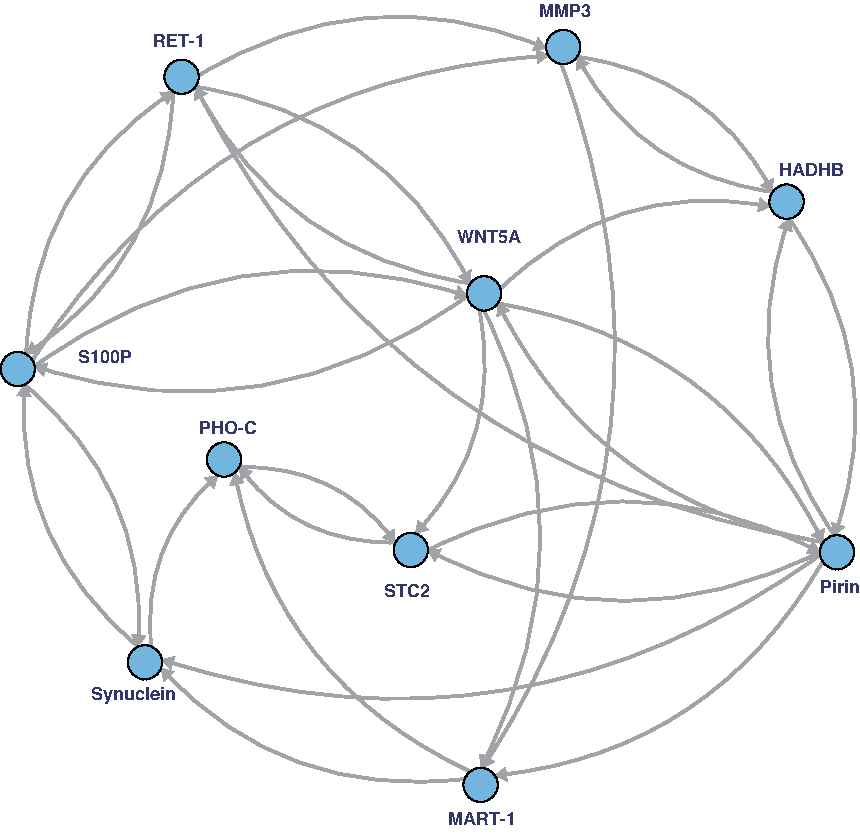
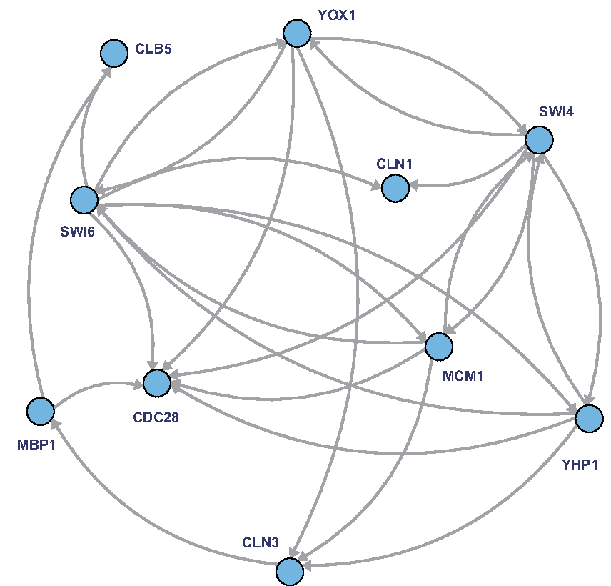
To show the effectiveness of the proposed algorithm, we used artificial time-course gene expression data from two synthetic networks of WNT5A (Kim et al., 2002) and a yeast cell cycle network (Kanehisa et al., 2012) as illustrated in Figures 4 and 5, respectively. For each network, we generated two time-courses consisting of \documentclass{aastex}\usepackage{amsbsy}\usepackage{amsfonts}\usepackage{amssymb}\usepackage{bm}\usepackage{mathrsfs}\usepackage{pifont}\usepackage{stmaryrd}\usepackage{textcomp}\usepackage{portland, xspace}\usepackage{amsmath, amsxtra}\pagestyle{empty}\DeclareMathSizes{10}{9}{7}{6}\begin{document} $${\cal T} = \{1 , 2 , \ldots , 30 \} $$ \end{document} and \documentclass{aastex}\usepackage{amsbsy}\usepackage{amsfonts}\usepackage{amssymb}\usepackage{bm}\usepackage{mathrsfs}\usepackage{pifont}\usepackage{stmaryrd}\usepackage{textcomp}\usepackage{portland, xspace}\usepackage{amsmath, amsxtra}\pagestyle{empty}\DeclareMathSizes{10}{9}{7}{6}\begin{document} $$\{1 , 2 , \ldots , 10 , 12 , \ldots , 30 \} $$ \end{document} by using Equations (3) and (4). For Equation (3), the values of the parameters were determined between 0 and 1, and the system noise was according to Gaussian distribution with a mean of 0 and a variance of 0.1. In Equation (4), Gaussian observational noise with a mean of 0 and a variance of 0.3 were added to these artificial data. Note that the networks were used for the performance comparison in the previous study (Nakajima et al., 2012).

FIG. 4.

A real biological network, termed WNT5A network (Kim et al., 2002), used for the comparison analysis. Based on the network, the original networks are generated by randomly adding and deleting five edges.

FIG. 5.

A real biological network of yeast cell cycle from the KEGG database (Nakajima et al., 2012; Kanehisa et al., 2012) used for comparison analysis. Based on the network, the original networks are generated by randomly adding and deleting five edges.

For this comparison, we applied (a) the proposed method, (b) a regression-based method (DPLSQ) (Nakajima et al., 2012), (c) DPLSQ with BIC (Schwarz, 1978), and (d) Akaike information criterion (AIC) (Akaike, 1974) to the data sets. Here, since DPLSQ is based only on the least-square errors, it may infer many false positives. Then, we modified the algorithm to use BIC and AIC; r in the proposed algorithm is set 3.

For each data set, 10 trials were executed, for each of which the true network of Figures 4 and 5 is randomly modified and given as an original network. Thus, a network obtained by adding and deleting five edges from the true network was given as an original network and then (a)–(d) were applied to obtain the true network. We evaluated the average performance of true positive (TP), false positive (FP), true negative (TN), false negative (FN), precision rate \documentclass{aastex}\usepackage{amsbsy}\usepackage{amsfonts}\usepackage{amssymb}\usepackage{bm}\usepackage{mathrsfs}\usepackage{pifont}\usepackage{stmaryrd}\usepackage{textcomp}\usepackage{portland, xspace}\usepackage{amsmath, amsxtra}\pagestyle{empty}\DeclareMathSizes{10}{9}{7}{6}\begin{document} $$(PR = {\frac {\rm TP} {\rm TP + FP}})$$ \end{document} , recall rate \documentclass{aastex}\usepackage{amsbsy}\usepackage{amsfonts}\usepackage{amssymb}\usepackage{bm}\usepackage{mathrsfs}\usepackage{pifont}\usepackage{stmaryrd}\usepackage{textcomp}\usepackage{portland, xspace}\usepackage{amsmath, amsxtra}\pagestyle{empty}\DeclareMathSizes{10}{9}{7}{6}\begin{document} $$(RR = {\frac {\rm TP} {\rm TP + FN}})$$ \end{document} , and F-measure \documentclass{aastex}\usepackage{amsbsy}\usepackage{amsfonts}\usepackage{amssymb}\usepackage{bm}\usepackage{mathrsfs}\usepackage{pifont}\usepackage{stmaryrd}\usepackage{textcomp}\usepackage{portland, xspace}\usepackage{amsmath, amsxtra}\pagestyle{empty}\DeclareMathSizes{10}{9}{7}{6}\begin{document} $$(= {\frac {\rm 2PR \cdot RR} {\rm PR + RR}})$$ \end{document} over 10 trials for each set of data. In contrast to the usual way, we counted TP when an altered edge was successfully improved as the true model, FN when an altered edge was not improved, and FP when an edge in the true model was changed in the improved model. The results of using the four time-courses are summarized in Tables 1 –4 (the proposed method is noted as “UKF-Completion”), respectively. These results clearly show that the proposed algorithm has the highest performance as compared to the other methods for all data sets. In particular, for non-equally spaced time-point data, the proposed method could better infer true regulations than the previous methods since our approach utilizes the hidden state and can handle nonobservational time points.

Table 1.

Comparison of the Proposed Method and DPLSQ Using Equally Spaced Artificial Data from WNT5A Network

	PR	RR	F-measure	TP	FP	TN	FN
DPLSQ	0.580	0.290	0.386	2.9	2.1	87.9	7.1
DPLSQ (BIC)	0.677	0.670	0.673	6.7	3.2	86.8	3.3
DPLSQ (AIC)	0.700	0.650	0.673	6.5	2.8	87.2	3.5
UKF-Completion	0.760	0.760	0.760	7.6	2.4	87.6	2.4

PR, precision rate; RR, recall rate; TP, true positive; FP, false positive; TN, true negative; FN, false negative; BIC, Bayesian information criterion; AIC, Akaike information criterion; UKF, unscented Kalman filter.

Table 2.

Comparison of the Proposed Method and DPLSQ Using Non-equally Spaced Artificial Data from WNT5A Network

	PR	RR	F-measure	TP	FP	TN	FN
DPLSQ	0.540	0.270	0.360	2.7	2.3	87.7	7.3
DPLSQ (BIC)	0.520	0.520	0.520	5.2	4.8	85.2	4.8
DPLSQ (AIC)	0.523	0.49	0.506	4.9	4.5	85.5	5.1
UKF-Completion	0.720	0.720	0.720	7.2	2.8	87.2	2.8

Table 3.

Comparison of the Proposed Method and DPLSQ Using Equally Spaced Artificial Data from a Yeast Cell Cycle Network

	PR	RR	F-measure	TP	FP	TN	FN
DPLSQ	0.600	0.300	0.400	3.0	2.0	88.0	7.0
DPLSQ (BIC)	0.597	0.590	0.593	5.9	4.0	86.0	4.1
DPLSQ (AIC)	0.600	0.600	0.600	6.0	4.0	86.0	4.0
UKF-completion	0.650	0.650	0.650	6.5	3.5	86.5	3.5

Table 4.

Comparison of the Proposed Method and DPLSQ Using Non-equally Spaced Artificial Data from a Yeast Cell Cycle Network

	PR	RR	F-measure	TP	FP	TN	FN
DPLSQ	0.475	0.238	0.317	2.4	2.6	87.4	7.6
DPLSQ (BIC)	0.413	0.413	0.413	4.1	5.9	84.1	5.9
DPLSQ (AIC)	0.413	0.413	0.413	4.1	5.9	84.1	5.9
UKF-Completion	0.588	0.588	0.588	5.9	4.1	85.9	4.1

3.2. Real data analysis using the yeast cell cycle network

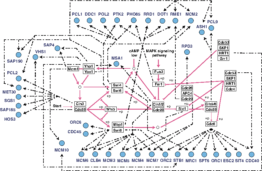
As an application example of improving and extending literature-based networks, we dealt with a yeast cell-cycle network from KEGG (Kanehisa et al., 2012) and used the corresponding observational data (Spellman et al., 1998). By using time-course data including 25 genes of which regulatory relationships are represented as red arrows in Figure 6, and considering this as an original network, we attempted to improve the network. However, since the network is classical and highly reliable in KEGG database, we focused on the extension of the network using additional genes. Thus, we considered the network consisting of these 25 genes and 38 additional candidate genes, which can have functions related to a yeast cell cycle pathway, from the Saccharomyces Genome Database (SGD) (Cherry et al., 2012). We did not set prior regulatory structure to these 38 genes and extended the KEGG-based network consisting of 25 genes by adding regulations to these 38 genes (del_max = 0).

FIG. 6.

A part of a yeast cell cycle network, and candidate genes for extending the network. The KEGG-based regulatory network consisting of 25 genes is drawn as rectangles (gene) and red arrows (regulation), and newly estimated relationships are drawn as circles (gene) and black chained arrows (regulation).

Consequently, 38 candidate genes were integrated in the KEGG-based yeast cell cycle network as illustrated in Figure 6. In this figure, the KEGG-based regulatory network consisting of 25 genes was drawn as rectangles (gene) and red arrows (regulation), and newly estimated relationships were drawn as circles (gene) and black chained arrows (regulation). Interestingly, there exist many combinatorial regulations of which regulated genes have more than two regulations. Since these regulations can have nonzero values of the combinatorial effect b_i_,(j,k), the results may not be obtained by linear models. Furthermore, some genes, such as YOX1 and Cdc6, become hub genes regulating many other genes, and they are known as upper stream genes regulating downstream genes on the KEGG database. These results show the possibility of the causal relationships between them.

4. Conclusion

We proposed a genomic data assimilation schema using a nonlinear simulation model for improving and extending literature-based networks. The method can efficiently estimate parameter values of a simulation model by using the EM-algorithm with UKF. Furthermore, the proposed algorithm avoids evaluating all possible candidates that are constructed by modifying the original network and selects only plausible ones through measuring the effectiveness when modifying the regulation of the current network for the data. Therefore, this schema makes it possible to deal with many candidate networks and finds better networks for the data.

The performance of this approach was demonstrated by implementing artificial simulation data from real biological networks termed WNT5A and a yeast cell cycle network. Consequently, our proposed method can evaluate GRNs more accurately than could a previously developed method (DPLSQ). In particular, since our method is based on the state space representation using the hidden state for representing gene regulatory dynamics, the flexibility for the observational data, that is, which can handle observational data with non-equally spaced time points, can be ensured. These results indicated the high performance and adaptability of the proposed method to improve and extend the original network using time-course observational data. As an application example, using a part of a well-investigated yeast cell-cycle network from KEGG, we applied the proposed method to extend the network by integrating additional candidate genes from SGD (Cherry et al., 2012). Interestingly, we found hub genes regulating candidate genes that are indicated as upstream genes in KEGG database. Since these are biologically related candidates of the original networks, these extensions might be true regulations and thus should be confirmed by biological experiments.

Footnotes

Acknowledgments

The super-computing resource was provided by the Human Genome Center, the Institute of Medical Science, the University of Tokyo.

This work was partly supported by Grant-in-Aid for JSPS Fellows Number 24-9639.

Author Disclosure Statement

No competing financial interests exist.

References

Akaike

1974. A new look at the statistical model identification. IEEE Transactions on Automatic Control, 19, 716–723.

Akutsu

, Tamura

, and Horimoto

2009. Completing networks using observed data, 126–140. In Gavalda

, Lugosi

, Zeugmann

, et al., eds. Algorithmic Learning Theory, Volume 5809, Lecture Notes in Computer Science. Springer, Berlin Heidelberg.

Asif

H.M.S.

, and Sanguinetti

2011. Large-scale learning of combinatorial transcriptional dynamics from gene expression. Bioinformatics, 27, 1277–1283.

Beal

M.J.

, Falciani

, Ghahramani

, Rangel

, and Wild

D.L.

2005. A Bayesian approach to reconstructing genetic regulatory networks with hidden factors. Bioinformatics, 21, 349–356.

Cherry

J.M.

, Hong

E.L.

, Amundsen

, et al. 2012. Saccharomyces genome database: the genomics resource of budding yeast. Nucleic Acids Res., 40, 700–705.

Chow

S.-M.

, Ferrer

, and Nesselroade

J.R.

2007. An unscented kalman filter approach to the estimation of nonlinear dynamical systems models. Multivariate Behavioral Research, 42, 283–321.

Dempster

A.P.

, Laird

N.M.

, and Rubin

D.B.

1977. Maximum likelihood from incomplete data via the EM algorithm. Journal of the Royal Statistical Society: Series B, 39, 1–38.

Friedman

, Hastie

, and Tibshirani

2007. Sparse inverse covariance estimation with the graphical lasso. Biostatistics, 9, 432–441.

Hasegawa

, Nagasaki

, Yamaguchi

, et al. 2014. An efficient method of exploring simulation models by assimilating literature and biological observational data. Biosystems, 121, 54–66.

10.

Hasegawa

, Yamaguchi

, Nagasaki

, et al. 2011. Comprehensive pharmacogenomic pathway screening by data assimilation. Proceedings of the 7th International Conference on Bioinformatics Research and Applications, ISBRA 11, 160–171. Springer-Verlag, Berlin, Heidelberg.

11.

Hirose

, Yoshida

, Imoto

, 2008. Statistical inference of transcriptional module-based gene networks from time course gene expression profiles by using state space models. Bioinformatics, 24, 932–942.

12.

Julier

2002. The scaled unscented transformation. American Control Conference, 2002, 6, 4555–4559.

13.

Julier

, and Uhlmann

2004. Unscented filtering and nonlinear estimation. Proceedings of the IEEE, 92, 401–422.

14.

Julier

, Uhlmann

, and Durrant-Whyte

2000. A new method for the nonlinear transformation of means and covariances in filters and estimators. IEEE Transactions on Automatic Control, 45, 477–482.

15.

Julier

S.J.

, and Uhlmann

J.K.

1997. A new extension of the kalman filter to nonlinear systems. Proc. of AeroSense: The 11th Int. Symp. on Aerospace/Defense Sensing, Simulations and Controls, 182–193.

16.

Kalman

R.E.

1960. A new approach to linear filtering and prediction problems. Transactions of the ASME - Journal of Basic Engineering, 82 (Series D), 35–45.

17.

Kanehisa

, Goto

, Sato

, et al. 2012. KEGG for integration and interpretation of large-scale molecular data sets. Nucleic Acids Res., 40, D109–D114.

18.

Kim

, Li

, Dougherty

E.R.

, et al. 2002. Can Markov chain models mimic biological regulation?. Journal of Biological Systems, 10, 337–357.

19.

Kitagawa

1998. A self-organizing state-space model. J. Am. Stat. Assoc., 93, 1203–1215.

20.

Koh

C.H.H.

, Nagasaki

, Saito

, et al. 2010. DA 1.0: parameter estimation of biological pathways using data assimilation approach. Bioinformatics, 26, 1794–1796.

21.

Kojima

, Yamaguchi

, Imoto

, et al. 2010. A state space representation of var models with sparse learning for dynamic gene networks. International Conference on Genome Informatics, 22, 56–68.

22.

Lillacci

, and Khammash

2010. Parameter estimation and model selection in computational biology. PLoS Comput. Biol., 6, e1000696.

23.

Liu

, and Niranjan

2012. State and parameter estimation of the heat shock response system using kalman and particle filters. Bioinformatics, 28, 1501–1507.

24.

Mahdi

, Madduri

A.S.

, Wang

, et al. 2012. Empirical Bayes conditional independence graphs for regulatory network recovery. Bioinformatics, 28, 2029–2036.

25.

Murtuza Baker

, Poskar

C.H.

, Schreiber

, and Junker

B.H.

2013. An improved constraint filtering technique for inferring hidden states and parameters of a biological model. Bioinformatics, 29, 1052–1059.

26.

Nagasaki

, Yamaguchi

, Yoshida

, 2006. Genomic data assimilation for estimating hybrid functional petri net from time-course gene expression data. Genome Informatics, 17, 46–61.

27.

Nakajima

, Tamura

, Yamanishi

, Horimoto

, and Akutsu

2012. Network completion using dynamic programming and least-squares fitting. Scientific World Journal, 2012.

28.

Nakamura

, Yoshida

, Nagasaki

, et al. 2009. Parameter estimation of in silico biological pathways with particle filtering toward a petascale computing. Pacific Symposium on Biocomputing 2009, 14, 227–238.

29.

Opper

, and Sanguinetti

2010. Learning combinatorial transcriptional dynamics from gene expression data. Bioinformatics, 26, 1623–1629.

30.

Quach

, Brunel

, and d'Alche Buc

2007. Estimating parameters and hidden variables in non-linear state-space models based on odes for biological networks inference. Bioinformatics, 23, 3209–3216.

31.

Rangel

, Angus

, Ghahramani

, et al. 2004. Modeling t-cell activation using gene expression profiling and state-space models. Bioinformatics, 20, 1361–1372.

32.

Rogers

, Khanin

, and Girolami

2007. Bayesian model-based inference of transcription factor activity. BMC Bioinformatics, 8 (Suppl).

33.

Sarkka

2008. Unscented rauch–tung–striebel smoother. IEEE Transactions on Automatic Control, 53, 845–849.

34.

Savageau

M.A.

1969. Biochemical systems analysis: II. The steady-state solutions for an n-pool system using a power-law approximation. J. Theor. Biol., 25, 370–379.

35.

Savageau

M.A.

, and Voit

E.O.

1987. Recasting nonlinear differential equations as s-systems: a canonical nonlinear form. Math. Biosci., 87, 83–115.

36.

Schwarz

1978. Estimating the dimension of a model. The Annals of Statistics, 6, 461–464.

37.

Spellman

P.T.

, Sherlock

, Zhang

M.Q.

, 1998. Comprehensive identification of cell cycle-regulated genes of the yeast saccharomyces cerevisiae by microarray hybridization. Mol. Biol. Cell. 9, 3273–3297.

38.

Wang

, Cherry

J.M.

, Nochomovitz

, 2005. Inference of combinatorial regulation in yeast transcriptional networks: A case study of sporulation. Proceedings of the National Academy of Sciences of the United States of America, 102, 1998–2003.

39.

Watanabe

, Seno

, Takenaka

, and Matsuda

2012. An estimation method for inference of gene regulatory network using Bayesian network with uniting of partial problems. BMC Genomics., 13, S12.