Probabilistic Generation of Random Networks Taking into Account Information on Motifs Occurrence

Abstract

Because of the huge number of graphs possible even with a small number of nodes, inference on network structure is known to be a challenging problem. Generating large random directed graphs with prescribed probabilities of occurrences of some meaningful patterns (motifs) is also difficult. We show how to generate such random graphs according to a formal probabilistic representation, using fast Markov chain Monte Carlo methods to sample them. As an illustration, we generate realistic graphs with several hundred nodes mimicking a gene transcription interaction network in Escherichia coli.

1. Introduction

Graph models are essential tools for understanding and modeling complex systems of interacting variables or agents (Albert and Barabási, 2002). The global features of social, telecommunication, or biological networks can only be analyzed with correspondingly large graph models. Such models consist of bonds (edges) indicating relationships between agents (nodes), with parameters quantifying the strength of the bonds. Over the years, graph models have been extensively studied both in theory (see, among others, Lauritzen, 1996) and in methodology (Whittaker, 1990) in different scientific areas, such as statistical physics (Gibbs, 1902), genetics (Wright, 1921), economics (Wold, 1954), or social sciences (Blalock, 1971). When there is no ambiguity about the links between nodes and their interactions' strengths, complex systems are well described by deterministic networks. In the presence of ambiguity about the system, probabilistic graphs are usually considered. In that case, bonds represent stochastic links between nodes and their parameters specify conditional distributions. Probabilistic graphs offer a natural framework for statistical inference and knowledge integration. For example, in communication engineering, we may want to know what conditions the robustness of a network; in systems biology we may be interested in understanding how genes control each other.

The theory of random graphs was initiated by Erdös and Rényi in a series of papers (Erdös and Rényi, 1959, 1960, 1961) in which they proposed to generate a random graph with a given number of labeled nodes by connecting every pair of nodes with probability \documentclass{aastex}\usepackage{amsbsy}\usepackage{amsfonts}\usepackage{amssymb}\usepackage{bm}\usepackage{mathrsfs}\usepackage{pifont}\usepackage{stmaryrd}\usepackage{textcomp}\usepackage{portland, xspace}\usepackage{amsmath, amsxtra}\pagestyle{empty}\DeclareMathSizes{10}{9}{7}{6}\begin{document} $$p ( p \in ( 0 , 1 ) )$$ \end{document} . The main goal of random graph theory has been to determine at which connection probability p a particular property of a graph will most likely emerge. One of the first properties studied by Erdös and Rényi is the appearance of given subgraphs like cliques, triangles, etc. In some sense, the question they have addressed is relative to the structure/topology on a graph. In many settings, interest focuses first on the structure of a graph, and the question arose of whether the random graphs proposed by Erdös and Rényi were able to display specific structures of real complex networks. Over the past few years, there has been a growing interest in investigating and developing new tools and measures able to capture specific properties of real networks. Among such properties are the degree distribution, corresponding to the probability P(k) that a node in the network is connected with k other nodes (Albert et al., 2000; Leskovec et al., 2010), small-world properties (Watts and Strogatz, 1998) in which most nodes are not neighbors of one another, or the node clustering coefficient (Watts and Strogatz, 1998).

Nevertheless, inference about network structures remains difficult because of the extremely large number of possible graphs, even with a modest number of nodes (Markowetz and Spang, 2007). Estimating the amount of data needed to recover the structure of a graph is also difficult, but it is clear at least in biology that most of the current experimental designs are insufficiently powerful for that aim. In such a context, every bit of information counts. Still in biology, the relevant scientific literature indicates that all graphs are not equally plausible, some being a priori more likely than others. Accounting for prior knowledge is well formalized in Bayesian statistics (Robert, 2001), but the probabilistic representation of such knowledge is still a question. Mukherjee and Speed (2008) have recently proposed a set of informative priors for network structure inference. More precisely, they have considered priors able to capture information relative to the existence of edges, degree distribution, or sparsity structure in Bayesian networks, that is, acyclic directed graph models.

Network motifs are patterns (subgraphs) that recur within a network much more often than expected for random graphs (Milo et al., 2002). It has been shown that gene transcription regulation networks, for example, in the bacteria Escherichia coli, contain a small set of network motifs (see Alon, 2007, and references therein), suggesting that such motifs are basic building blocks of transcription networks. An important aspect of network topology inference is therefore to include the probability of occurrence of such network motifs (see Janson et al., 2000, for an overview).

In this article, we address precisely that question. We extend the approach of Mukherjee and Speed (2008) by relaxing the acyclicity requirement that characterizes Bayesian networks and proposing rigorous probabilistic representations of a priori information on pairwise links, degree node distribution, and network motifs (see section 2). We use Markov chain Monte Carlo (MCMC) simulations to sample networks satisfying those joint distributions for moderately large networks (several hundred to thousands of nodes). Such random networks can be used as priors for formal inference, after updating with data in a Bayesian framework. They can also be used for pure simulation purposes, for example, for methods or software testing. We do not deal with data and associated likelihood (or “score”) functions, but focus on probabilities. Our distributions, however, are entirely compatible with any score function and can be used for inference, in particular in a Bayesian framework. Section 5 is devoted to simulations; as an illustration, we generate realistic graphs mimicking a gene transcription interaction network in E. coli. The weight of the various proposed priors is examined. We end the article with a discussion of those results (Section 6).

2. Graph Models for Networks

A graph model simply consists of nodes (vertices) connected by edges (Wilson, 2012). The nodes often represent physical entities (people, genes, servers… ), and the edges represent links or dependencies between them (“is a friend,” “controls,” “is physically connected to,” … ). Nodes can be assigned attributes (e.g., “on,” “off”) that can depend in turn on the attributes of the nodes to which they are connected. The edges may also have attributes influencing those of the nodes they connect. Edges may be “undirected” or “directed,” the latter case (often noted by an arrow) introducing an asymmetry between the two nodes. For example, an arrow from node i to node j may indicate that i controls j, the reverse not being true. Directed edges can in turn be signed, indicating a positive or negative control, etc. Finally, graph models may have global features imposed to them. For example, we may impose no unconnected node. A commonly imposed feature is “acyclicity.” In that case, the graph model cannot contain any path (succession of edges) linking any node to itself, and in particular no “auto-loop” edge from a node to itself. In the case of directed edges, paths are understood to follow the directions of the edges. A particular class of such acyclic directed graph models, Bayesian networks, has a clear probabilistic interpretation and is easily amenable to inference about network structure or parameters (Neapolitan, 2003).

Since we are interested in generating general graphs, in particular those describing genetic regulatory systems, we consider directed graphs that may be cyclic (see De Jong, 2002, for an overview of genetic regulatory networks modeling). More precisely, our graphs are composed of labeled nodes with directed edges. There can be two reverse edges between any two nodes and auto-loops are allowed.

3. Informative Priors on Networks

Let G be a graph described by a set \documentclass{aastex}\usepackage{amsbsy}\usepackage{amsfonts}\usepackage{amssymb}\usepackage{bm}\usepackage{mathrsfs}\usepackage{pifont}\usepackage{stmaryrd}\usepackage{textcomp}\usepackage{portland, xspace}\usepackage{amsmath, amsxtra}\pagestyle{empty}\DeclareMathSizes{10}{9}{7}{6}\begin{document} $$V ( G ) = \{ v_1 , \ldots , v_n \} $$ \end{document} of n vertices (n ≥ 2) and a set \documentclass{aastex}\usepackage{amsbsy}\usepackage{amsfonts}\usepackage{amssymb}\usepackage{bm}\usepackage{mathrsfs}\usepackage{pifont}\usepackage{stmaryrd}\usepackage{textcomp}\usepackage{portland, xspace}\usepackage{amsmath, amsxtra}\pagestyle{empty}\DeclareMathSizes{10}{9}{7}{6}\begin{document} $$E ( G ) = \{ e_{i , j}: ( i , j ) \in \{ 1 , \ldots , n \} \times \{ 1 , \ldots , n \} \} $$ \end{document} of directed edges and auto-loops. G may be described by its adjacency matrix A, an (n × n)-matrix whose generic term is given by \documentclass{aastex}\usepackage{amsbsy}\usepackage{amsfonts}\usepackage{amssymb}\usepackage{bm}\usepackage{mathrsfs}\usepackage{pifont}\usepackage{stmaryrd}\usepackage{textcomp}\usepackage{portland, xspace}\usepackage{amsmath, amsxtra}\pagestyle{empty}\DeclareMathSizes{10}{9}{7}{6}\begin{document} \begin{align*}a_{i , j} = \begin{cases} 1 \qquad \hbox{if the edge} \ e_{i , j} \ { \rm exists} \\ 0 \qquad \hbox{otherwise}\end{cases}.\end{align*} \end{document}

Incomplete a priori knowledge on such a graph can be described by a statistical distribution. Given n, the number of nodes of G, we propose to include three levels of complexity in that distribution. It is only mandatory to define the first level, which does not reflect any specific structure except for the probability of presence of individual edges (section 3.1). We then refine it by including information on the degree distribution (section 3.2). The next step is to incorporate information related to the occurrences of subnetwork motifs (section 3.3).

3.1. Priors on individual Edges

As in the random graphs considered by Erdös and Rényi, prior knowledge on each individual edge can be conveniently modeled by a Bernoulli distribution, assigning probability p_i,j to the existence of a directed edge from node i to node j, that is, \documentclass{aastex}\usepackage{amsbsy}\usepackage{amsfonts}\usepackage{amssymb}\usepackage{bm}\usepackage{mathrsfs}\usepackage{pifont}\usepackage{stmaryrd}\usepackage{textcomp}\usepackage{portland, xspace}\usepackage{amsmath, amsxtra}\pagestyle{empty}\DeclareMathSizes{10}{9}{7}{6}\begin{document} $$e_{i , j} \sim B ( p_{i , j} ) \ \hbox{for all} \ ( i , j ) \in \{ 1 , \ldots , n \} \times \{ 1 , \ldots , n \} $$ \end{document} . In this context, the adjacency matrix A related to a graph G with n nodes becomes A = (e_i,j)_{{1≤i,j,≤n}}.

For a graph of a given size n, there are n² individual pairwise possible links in the cyclic case and at most n²−n in the acyclic case (auto-loops being ruled out by definition). Specifying the complete set of edge priors requires the definition of an n × n matrix P = (p_i,j)_1≤i,j≤n (with a null diagonal in the acyclic case). If the pairwise links are supposed to be independent, the probability distribution for the entire graph G is therefore \documentclass{aastex}\usepackage{amsbsy}\usepackage{amsfonts}\usepackage{amssymb}\usepackage{bm}\usepackage{mathrsfs}\usepackage{pifont}\usepackage{stmaryrd}\usepackage{textcomp}\usepackage{portland, xspace}\usepackage{amsmath, amsxtra}\pagestyle{empty}\DeclareMathSizes{10}{9}{7}{6}\begin{document} \begin{align*}P_{Bern , G} = \prod_{i , j = 1}^{n} p_{i , j}^{e_{i , j}} ( 1 - p_{i , j} ) ^{e_{i , j} - 1}. \tag{1}\end{align*} \end{document}

There are various ways to choose or elicit values for the individual prior probabilities p_i,j, which we will further discuss in section 5, but intuitively they are related to the weight of the prior evidence (e.g., p-values, Bernard and Hartemink, 2005), we have on the existence of given edges. Other distributions could be used, such as a multinomial if we had chosen to give a sign to the edges (to indicate positive or negative interactions, for example). But the principle would remain the same, and in the absence of precise prior information, a Bernoulli prior is probably all we can specify.

3.2. Priors on degrees' counts

The degree deg(v) of a vertex v is the total number of edges to which vertex v participates. The degree distribution of a graph G is a function P(d) expressed in terms of \documentclass{aastex}\usepackage{amsbsy}\usepackage{amsfonts}\usepackage{amssymb}\usepackage{bm}\usepackage{mathrsfs}\usepackage{pifont}\usepackage{stmaryrd}\usepackage{textcomp}\usepackage{portland, xspace}\usepackage{amsmath, amsxtra}\pagestyle{empty}\DeclareMathSizes{10}{9}{7}{6}\begin{document} $$\mid \{ v \in V ( G ) : deg ( v ) = d \} \mid$$ \end{document} , the total number of vertices having degree d. In many biological networks (Jeong et al., 2000), it appears that the degree distribution has a power-law tail, which means that P(d) ∝ d^−γ, with γ > 0. Such networks are called scale-free (Barabási and Albert, 1999). Then, we define the probability distribution of a graph G as follows \documentclass{aastex}\usepackage{amsbsy}\usepackage{amsfonts}\usepackage{amssymb}\usepackage{bm}\usepackage{mathrsfs}\usepackage{pifont}\usepackage{stmaryrd}\usepackage{textcomp}\usepackage{portland, xspace}\usepackage{amsmath, amsxtra}\pagestyle{empty}\DeclareMathSizes{10}{9}{7}{6}\begin{document} \begin{align*}P_{deg , G} \propto P_{Bern , G} \times \prod_{i = 1}^{n} \left( \sum_{j \in \{ 1 , \ldots , n \} : \sum_j e_{i , j} > 0} e_{i , j} \right) ^{ - \gamma}. \tag{2}\end{align*} \end{document}

Since we do not impose that every node should be linked to another one, the degree distribution attributes implicitly a weight of one to any isolated node. It entails that the probability, with respect to degrees, of an empty graph (without any connection between its nodes) is one.

Here again, other distributions, even empirical (as defined by a histogram) and reflecting better the degree distribution of a given class of graphs, could be used if enough information was available.

3.3. Priors on motifs

One important local property of networks is the eventual occurrence of motifs. Motifs are defined here following Milo et al. (2002, 2004), Alon (2007), Shen-Orr et al. (2002), and Kashtan et al. (2004), as over-represented subgraphs compared to what is found in an Erdös and Rényi random graph. Some motifs have a notable importance in biological networks because they can carry out specific information-processing functions, and hence may help in understanding the global behavior of such networks (Masoudi-Nejad et al., 2012). For example, there are thirteen possible configurations for the relationships between three nodes (Fig. 1). Among the nondegenerate configurations, only the feed-forward loop (FFL, top row, first motif on the left, Fig. 1) has been found in the transcriptional regulation network of E. coli (Alon, 2007; Shen-Orr, 2002; Mangan et al., 2003). No feedback loop (FFB, top row, second motif on the left, Fig. 1) has been observed in E. coli. The FFL is one of the most studied network motifs in transcription interactions. It corresponds to a directed subgraph of three nodes (genes) such that one of them is regulated by the two others, which are linked. Given that each of the regulatory interactions can cause either an activation or a repression, there are eight subtypes of signed FFL, two of them occurring much more frequently than the other six in transcription networks (Mangan and Alon, 2003; Mangan et al., 2006).

FIG. 1.

The thirteen possible three-node motifs.

In this article, we consider network motifs with three nodes; auto-loops are not taken into account in such subgraphs. We define a motif distribution based on the proportion of FBL among all three-node loops. More precisely, for a graph G let us consider N₁ the number of FBL motifs and N₂ the number of FFL motifs and note they may be expressed in terms of (e_i,j)_{{1≤i,j≤n}} as follows, \documentclass{aastex}\usepackage{amsbsy}\usepackage{amsfonts}\usepackage{amssymb}\usepackage{bm}\usepackage{mathrsfs}\usepackage{pifont}\usepackage{stmaryrd}\usepackage{textcomp}\usepackage{portland, xspace}\usepackage{amsmath, amsxtra}\pagestyle{empty}\DeclareMathSizes{10}{9}{7}{6}\begin{document} \begin{align*}N_1 = \sum_{ ( i , j , k ) : i \neq j , k \neq j , i \neq k} e_{i , j} e_{j , k}e_{k , i} \ { \rm and} \ N_2 = \sum_{ ( i , j , k ) : i \neq j , k \neq j , i \neq k} e_{i , j} e_{j , k}e_{i , k}.\end{align*} \end{document}

For a graph G with a total number N₁+N₂ of motifs of type FBL and FFL, we place a beta-binomial probability with parameters u and v on N₁, BB(N₁|u, v, N₁+N₂). The prior for graph G is then \documentclass{aastex}\usepackage{amsbsy}\usepackage{amsfonts}\usepackage{amssymb}\usepackage{bm}\usepackage{mathrsfs}\usepackage{pifont}\usepackage{stmaryrd}\usepackage{textcomp}\usepackage{portland, xspace}\usepackage{amsmath, amsxtra}\pagestyle{empty}\DeclareMathSizes{10}{9}{7}{6}\begin{document} \begin{align*}P_ { Motif , G } \propto P_ { Bern , G } \times C_ { N_1 + N_2 } ^ { N_1 } \frac { B ( N_1 + u , N_2 + v ) } { B ( u , v ) } , \tag { 3 } \end{align*} \end{document}

where \documentclass{aastex}\usepackage{amsbsy}\usepackage{amsfonts}\usepackage{amssymb}\usepackage{bm}\usepackage{mathrsfs}\usepackage{pifont}\usepackage{stmaryrd}\usepackage{textcomp}\usepackage{portland, xspace}\usepackage{amsmath, amsxtra}\pagestyle{empty}\DeclareMathSizes{10}{9}{7}{6}\begin{document} $$C_{N_1 + N_2}^{N_1}$$ \end{document} is a binomial coefficient and B(·,·) denotes the beta function. The choice of a beta-binomial distribution is justified by the fact that we may not know the exact proportions of FFL and FBL, but simply have observations about the numbers of such loops in some actual network on which we base our prior. Obviously, as we will discuss later, other motifs could be tracked and entered in the definition of a graph probability, using a similar device.

3.4. Piecing together a global prior

In addition to the probabilities P_Bern,G, P_Deg,G, and P_Motif,G defined by Equations (1), (2), and (3) respectively, we consider one more graph distribution P_Total,G that combines all informative priors independently. Therefore, \documentclass{aastex}\usepackage{amsbsy}\usepackage{amsfonts}\usepackage{amssymb}\usepackage{bm}\usepackage{mathrsfs}\usepackage{pifont}\usepackage{stmaryrd}\usepackage{textcomp}\usepackage{portland, xspace}\usepackage{amsmath, amsxtra}\pagestyle{empty}\DeclareMathSizes{10}{9}{7}{6}\begin{document} \begin{align*} P_ { Total , G } \propto & \prod_ { i , j = 1 } ^ { n } p_ { i , j } ^ { e_ { i , j } } ( 1 - p_ { i , j } ) ^ { e_ { i , j } - 1 } \times \prod_ { i = 1 } ^n \left( \sum_ { j \in \{ 1 , \ldots , n \} : \sum_j e_ { i , j } > 0 } e_ { i , j } \right) ^ { - \gamma } \\ & \times C_ { N_1 + N_2 } ^ { N_1 } \frac { B ( N_1 + u , N_2 + v ) } { B ( u , v ) } . & ( 4 ) \end{align*} \end{document}

4. Sampling Random Graphs

Graph probabilities such as P_Total,G are only defined up to a multiplicative constant. In that case, a simple way to generate sample graphs according to that probability distribution is to use the Metropolis-Hasting sampler (see Casella and Robert, 2004). From a current graph G, with total probability P_Total,G (Eq. 4), a graph \documentclass{aastex}\usepackage{amsbsy}\usepackage{amsfonts}\usepackage{amssymb}\usepackage{bm}\usepackage{mathrsfs}\usepackage{pifont}\usepackage{stmaryrd}\usepackage{textcomp}\usepackage{portland, xspace}\usepackage{amsmath, amsxtra}\pagestyle{empty}\DeclareMathSizes{10}{9}{7}{6}\begin{document} $$\tilde {G}$$ \end{document} is proposed by first selecting two nodes, say v_i and v_j of G (v_i may be equal to v_j in case of auto-loops) and then by deciding on the presence of an edge from v_i and v_j by a random Bernoulli draw with edge probability p_i,j. That amounts to sampling \documentclass{aastex}\usepackage{amsbsy}\usepackage{amsfonts}\usepackage{amssymb}\usepackage{bm}\usepackage{mathrsfs}\usepackage{pifont}\usepackage{stmaryrd}\usepackage{textcomp}\usepackage{portland, xspace}\usepackage{amsmath, amsxtra}\pagestyle{empty}\DeclareMathSizes{10}{9}{7}{6}\begin{document} $$\tilde {G}$$ \end{document} from the Bernoulli prior on edges defined in Equation (1). The total probability \documentclass{aastex}\usepackage{amsbsy}\usepackage{amsfonts}\usepackage{amssymb}\usepackage{bm}\usepackage{mathrsfs}\usepackage{pifont}\usepackage{stmaryrd}\usepackage{textcomp}\usepackage{portland, xspace}\usepackage{amsmath, amsxtra}\pagestyle{empty}\DeclareMathSizes{10}{9}{7}{6}\begin{document} $$P_{Total , \tilde G}$$ \end{document} of \documentclass{aastex}\usepackage{amsbsy}\usepackage{amsfonts}\usepackage{amssymb}\usepackage{bm}\usepackage{mathrsfs}\usepackage{pifont}\usepackage{stmaryrd}\usepackage{textcomp}\usepackage{portland, xspace}\usepackage{amsmath, amsxtra}\pagestyle{empty}\DeclareMathSizes{10}{9}{7}{6}\begin{document} $$\tilde {G}$$ \end{document} is computed using Equation (4) and \documentclass{aastex}\usepackage{amsbsy}\usepackage{amsfonts}\usepackage{amssymb}\usepackage{bm}\usepackage{mathrsfs}\usepackage{pifont}\usepackage{stmaryrd}\usepackage{textcomp}\usepackage{portland, xspace}\usepackage{amsmath, amsxtra}\pagestyle{empty}\DeclareMathSizes{10}{9}{7}{6}\begin{document} $$\tilde {G}$$ \end{document} is accepted with a probability equal to min \documentclass{aastex}\usepackage{amsbsy}\usepackage{amsfonts}\usepackage{amssymb}\usepackage{bm}\usepackage{mathrsfs}\usepackage{pifont}\usepackage{stmaryrd}\usepackage{textcomp}\usepackage{portland, xspace}\usepackage{amsmath, amsxtra}\pagestyle{empty}\DeclareMathSizes{10}{9}{7}{6}\begin{document} $$( 1 , \frac { P_ { Total , \tilde { G } } } { P_ { Total , G } } )$$ \end{document} . In case of rejection, \documentclass{aastex}\usepackage{amsbsy}\usepackage{amsfonts}\usepackage{amssymb}\usepackage{bm}\usepackage{mathrsfs}\usepackage{pifont}\usepackage{stmaryrd}\usepackage{textcomp}\usepackage{portland, xspace}\usepackage{amsmath, amsxtra}\pagestyle{empty}\DeclareMathSizes{10}{9}{7}{6}\begin{document} $$\tilde {G}$$ \end{document} is discarded, and G is again the current sample (which implies that the same graph can be drawn several times in succession). The procedure is iterated as many times as it is needed to reach convergence in probability to the target distribution sought. Convergence can be checked by running several simulation chains and computing Gelman and Rubin's \documentclass{aastex}\usepackage{amsbsy}\usepackage{amsfonts}\usepackage{amssymb}\usepackage{bm}\usepackage{mathrsfs}\usepackage{pifont}\usepackage{stmaryrd}\usepackage{textcomp}\usepackage{portland, xspace}\usepackage{amsmath, amsxtra}\pagestyle{empty}\DeclareMathSizes{10}{9}{7}{6}\begin{document} $$\hat{R}$$ \end{document} criterion (Gelman and Rubin, 1992) on each element of the graphs' adjacency matrix, or by monitoring the degree distributions obtained, or the motif probabilities in those independent chains.

A C-language version of the algorithm has been implemented as a module of the free GNU MCSim software (Bois, 2009). That software was used for all the simulations presented here. Graphs were produced with R, version 2.14 (R Development Core Team, 2011).

5. Application To A Biological Network

Transcriptional regulatory networks orchestrate the gene expression of cells. In such networks, the nodes are operons (one or more genes transcribed on the same mRNA template). Edges go from operons encoding a transcription factor to operons directly regulated by that factor. Shen-Orr et al. (2002) developed and applied motif-detection algorithms to the transcriptional regulation network of E. coli. They extracted data from the RegulonDB transcriptional database (Salgado et al., 2013), and enhanced them with additional transcription factors and interactions described in the literature. We used here the latest version of the dataset (version 1.1, made publicly available by Dr. U. Alon).

A graph representation of the E. coli transcriptional regulatory network is shown in Figure 2. It contains 423 nodes, all connected, with 578 directed edges. That is actually only 0.32% of the number of possible edges, indicating that the network is sparse.

FIG. 2.

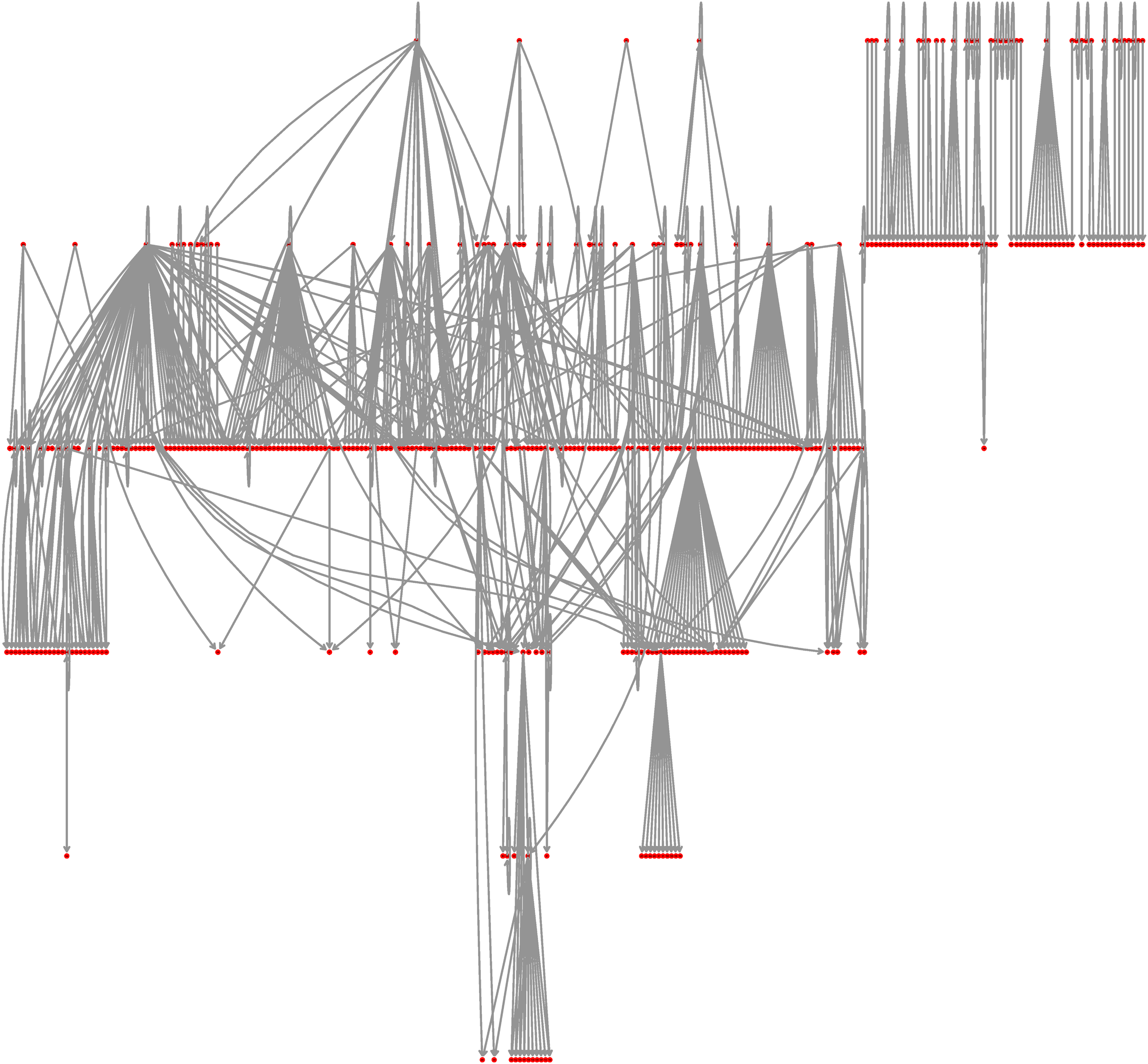
E. coli transcriptional regulatory network, as reported in Shen-Orr et al. (2002), with minor updates (see text).

We report here the results for Alon's full size network (of 423 nodes). We investigate here which elements of our prior knowledge on E. coli regulatory network features are the most important to simulate realistic networks.

In a first set of simulations we assigned “vague” priors to the edge probabilities, setting them all to the same value (equal to 578/423², i.e., 0.0032). With that prior, all connections are equally probable, and their expected number is equal to the one observed for E. coli. In E. coli the degree distribution follows approximately a power law with an exponent of 1.7 (Fig. 3), so we set γ to that value when the degree distribution was in effect. In addition, E. coli regulatory network is known to contains 42 FFLs and no FBL. To allow flexibility in the prior and allow some occurence of FBL motifs, we set Equation (3) parameter u to 2 and parameter v to 50 in our simulations. That implies an expected proportion of only 2% FBLs.

FIG. 3.

Degree distribution in E. coli actual transcriptional regulation network (in red) and in Monte-Carlo sampled networks (in black). An informative distribution on individual edges was used. The dip for high degrees is due to the mere absence of those degrees in the actual network (a deviation of reality from the power law assumption).

In the second set of simulations we use the same priors for degree distribution and motif frequencies, but used informative priors to individual edge probabilities; the edges reported by Alon et al. were assigned probability 0.95. Non reported, therefore hypothetical, edges were assigned probability 0.00016. Together those probabilities lead again to 578 expected edges.

In all cases, three MCMC chains of 2 billion iterations were run independently. Convergence of the edge probabilities (according to Gelman and Rubin's criterion) was always attained after at most 1 billion iterations. The degree distribution (e.g., Fig. 3) and motif frequencies (e.g., Fig. 4) also converged within that time frame. Results from the three independent chains basically overlap, except in the case of rare events (with frequencies less than 1 in 10,000), where Monte Carlo sampling uncertainty becomes noticeable. We therefore discarded systematically the first billion simulations and base all the following results on the second billion. We optimized our MCMC sampling C code and simulations are rather fast. Running 2 billion iterations to generate a random graph with 423 nodes takes about 2 minutes on a Intel Core 2 Duo machine clocked at 2.13 GHz. It takes actually little more time to sample graphs with a thousand nodes. Overall, the time it takes to update all the elements of the adjacency matrix is approximately proportional to the number of its elements, and therefore proportional to the square of the number of nodes for the graph considered. In our implementation, memory requirements are simply proportional to the number of nodes and minimal.

FIG. 4.

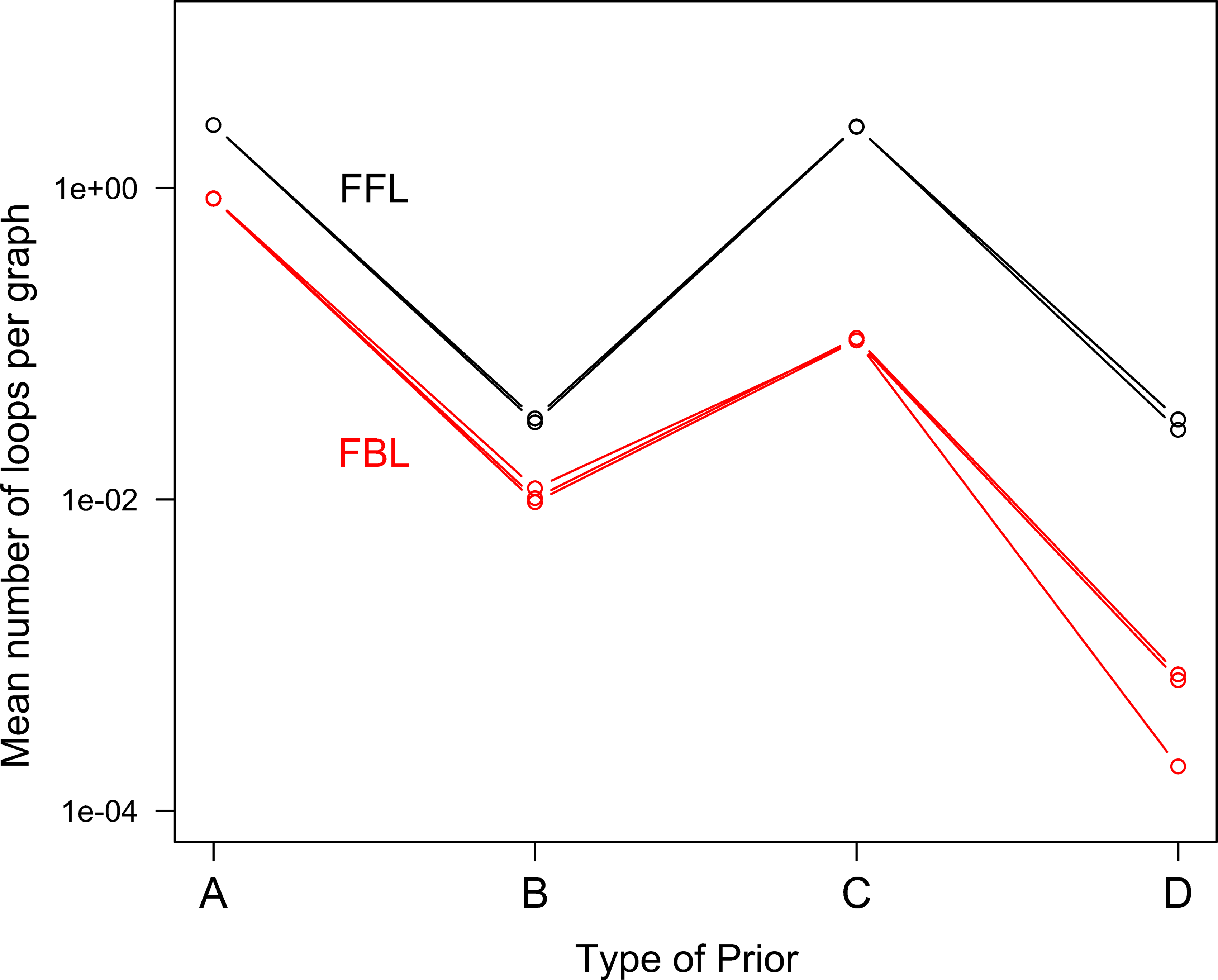
Motif frequencies in transcriptional regulation networks generated using a vague prior on individual edges. Types of priors are (A) prior on individual edges only; (B) prior on individual edges and degree distribution; (C) prior on individual edges and the proportion of feedback loops; and (D) all three priors together.

Figure 5 shows samples of networks generated using the above vague prior on individual edges. Used alone, that prior gives all edges the same probability and the resulting network has little structure, except that the expected number of edges is respected (Fig. 5A). The proportion of FBLs is 1/4, as expected in an unconstrained setting (there are two possible FBLs and six possible FFLs for each triplet of nodes). Adding the prior component on degree distribution imposes a major change in network shape. The number of edges is similar, but the structure becomes hierarchical (panel B). Placing a prior on the proportion of FBLs and FFLs, in addition to the prior on individual edges, has little visible impact on the structure (panel C), but the proportion of loops is now much lower and close to its expected value. Finally (panel D) putting the three priors together gives us again a hierarchical structure, but with the correct proportion of FBLs.

FIG. 5.

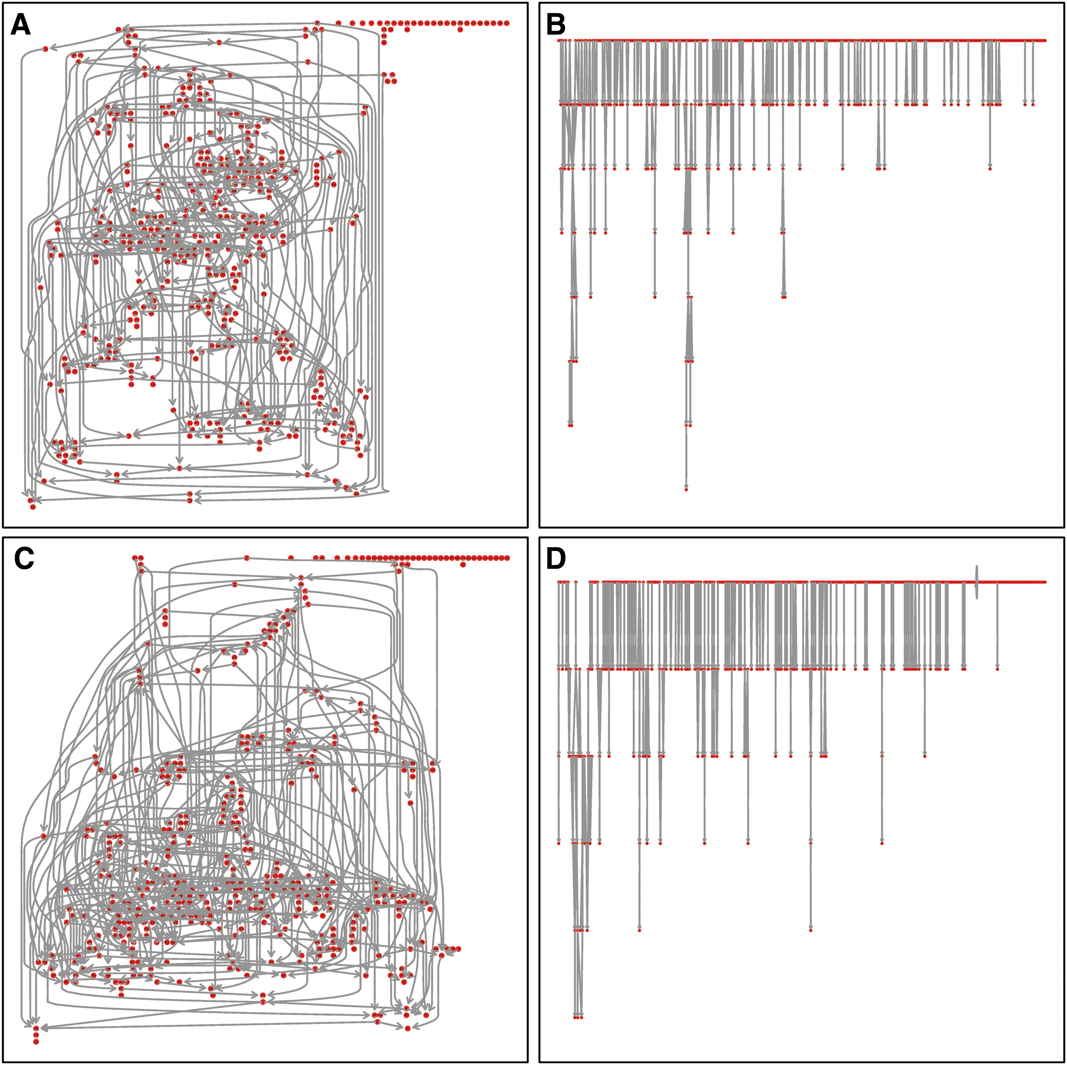
Transcriptional regulation networks generated using a vague prior on individual edges. There are 423 genes (red dots) in each network. (A) Prior on individual edges only; (B) prior on individual edges and degree distribution; (C) prior on individual edges and the proportion of feedback loops; and (D) all three priors together.

Figure 4 shows in more detail how the number of feedback and feed-forward loops is influenced by the specification of prior knowledge in the context of a vague specification of individual edge probabilities. The hierarchical structure imposed by the degree distribution (prior “B”) leads to a much lower number of loops, but without altering the ratio of FBLs to FFLs (25% in the case of prior “A” and “B”). In contrast, imposing a prior on the proportion of FBLs can later reduce both the ratio (4% in the case of prior “C” and 2% with prior “D”) and the number of loops in the network.

If we now turn to networks simulated with an informative prior on individual edges (Fig. 6) we see a striking difference with Figure 5. The structure of those networks, even if random, is quite close to the actual E. coli transcriptional regulation network (Fig. 2). The difference between the networks with a prior on degrees (B and D) or without (A and C) is now more subtle. Actually the prior on individual edges is strong enough to impose a correct distribution of degrees, even if the degree distribution is not specified (see Fig. 3). In that figure, a deviation of the actual number of degrees from the power law, for high degrees, can be observed and is well simulated. A similar behavior of degree distribution can be found in Dobrin et al. (2004). In Figure 6, the frequency of motifs is also controlled directly by the edge's probabilities. The number of FBLs is about constant at 1.5×10⁷, for approximately 3×10⁷ FFLs, hence a proportion of 0.05%. The differences between chains are small and all those results have a 5% CV.

FIG. 6.

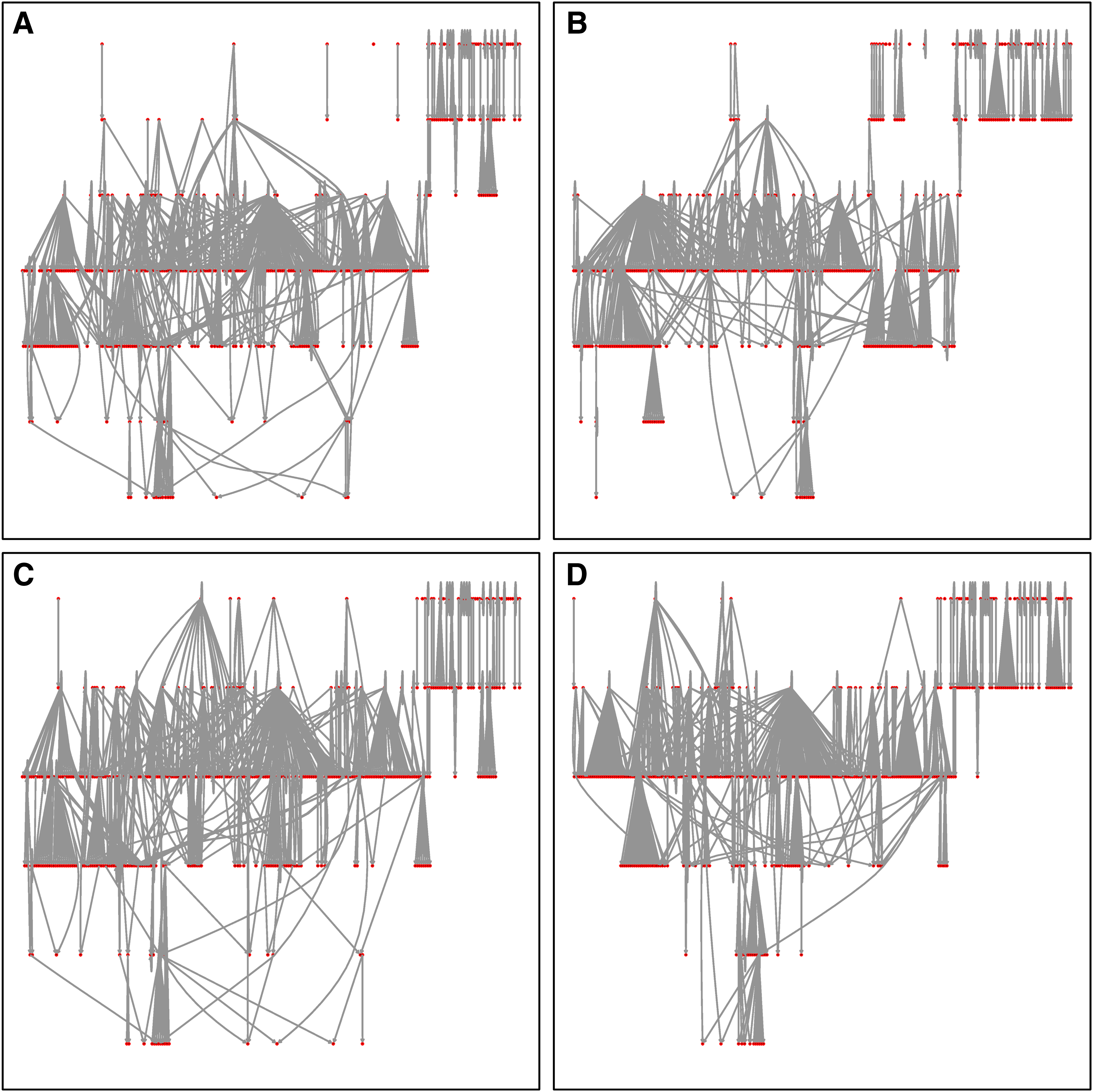
Transcriptional regulation networks generated using informative priors on individual edges (on the basis of the E. coli network). There are 423 genes (red dots) in each network. (A) Prior on individual edges only; (B) prior on individual edges and degree distribution; (C) prior on individual edges and the proportion of feedback loops; and (D) all three priors together.

6. Discussion

There are two important applications to the generation of semirandom graphs with known properties: (i). Simulating actual networks for hypothesis testing, software bench-marking, statistical power calculations, etc. (Van den Bulcke et al., 2006); and (ii.) assessing whether a graph is coherent with our prior knowledge in numerical data analytic methods such as Bayesian network modeling, Gaussian graphical methods, etc. Such methods, in their naive implementation, are known to suffer badly from the curse of dimensionality. However, prior knowledge about network structure increases daily, at least for biological networks, and a proper accounting of such knowledge is our only hope to redeem the curse we face.

We have extended here the results presented in Mukherjee and Speed (2008) by including a flexible specification of edge probability, via Bernoulli priors, and by defining a prior on network motifs. In doing so we have dropped the commonly used distance penalty from a prespecified reference network (whereby “distance” corresponds to the number of differing edges between a proposed graph and the reference graph). Such a distance penalty is simple to specify and compute, but has several drawbacks: It is quite coarse and does not give a weight to the various edges, while in fact we may be more or less certain about some of them. Therefore it treats in the same way edges known to be absent or present, and edges for which we do not know whether they are absent or present. Also, only one reference network is specified and this limits the number of questions we can ask. It is finally more an ad hoc penalty function than a proper distribution, although that may be seen as a purely technical argument. In any case, an edge-by-edge prior probability assignment is not much more difficult to specify, it can be simplified by giving default vague probability values if information is lacking, and can be quite powerful when information is available.

There are, however, cases where higher levels of structure are important. In fact, we can hypothesize that higher levels are more important than we usually suspect. That is the whole point of systems biology. Power law degree distribution is a well known characteristic of biological networks. The frequency of occurrence of particular network motifs is another point in case. Fascinating recent work has addressed the question of degree distribution (Leskovec et al., 2010), but the problem remains for motifs since no direct sampling or generative method is available in that case. We have shown here how to use MCMC sampling to obtain the desired random graphs, even for realistically large numbers of nodes. An important point is that a sample of random graphs is much more informative than a single approximate, or even “best,” estimate graph. With a single graph, all sense of uncertainty is lost, and only over-confidence is gained. Ensemble results are much more robust and useful, but they can be cumbersome and the question is how to best handle them.

Stochastic simulations also give insights about the relative weights of the various components of our prior knowledge. A first point is that prior knowledge about the probable number of edges, or at least about network sparsity, can strongly constrain the set of admissible networks. At least, that is the case when implemented in a form of Bernoulli priors on individual edges. Actually, more flexible priors (e.g., hierarchical) could be used instead of Bernoulli to allow more uncertainty about that expected number of edges. Specific knowledge about subsets of high probability, or conversely low probability, edges is also very informative. The degree distribution of a network may appear as a weak predictor of its structure since, for example, with a given number of nodes, two graphs with the same degree distribution may have completely different edge lists. However, we found that specifying a degree distribution has a visible impact on the network structure. Here again it would be easy to be more flexible about that distribution. Imposing a prior on the occurrence of specific motifs can be important in terms of functionality, but leads to more subtle modifications. Note however, that we imposed a distribution on the relative frequency of two loop motifs, rather than on their absolute number. That would be an easy extension, which could have profound consequences on the network structure. Overall, there are many variables with which the prior can play, and even potential conflicts between components of our prior knowledge, in particular if a strongly informative prior is placed on individual edges. Such conflicts can be hard to figure out without the help of simulations, because our intuition often fails in high dimension and in the case of graphs (Helbing, 2013). In that respect, the possibility to perform quickly billions of iterations for a network of sizes commensurable to those of genomes is encouraging. A word of caution is in order here, however; with 423 nodes, a billion simulations correspond to 10⁹ × 423⁻², that is, about 6000 full updates of the network. With 10⁴ nodes we might have to go to trillions of simulations to get to convergence, and this would currently take us a day and half of computation, although GPU computing, for example, could again increase speed.

To be more precise about the relative weight of the different priors would have required some evaluation of the number of possible graphs, or some form of enumeration of the number of different graphs sampled during stochastic simulations. However, there are, for example, 2¹⁷⁸⁹²⁹ different directed graphs with 423 nodes, and tracking the list of graphs sampled would entailed considerable time and memory capacity.

Obviously, it would be interesting to extend those results to the important problem of statistical learning of the network structure from data acquired in large scale genotyping or phenotyping studies, for example. In a Bayesian context, that simply entails the computation of a data likelihood function, or its marginalization. However, the models currently favored for that purpose: Gaussian graphical networks (Krumsiek et al., 2011; Liu et al., 2012) and Bayesian networks (Mukherjee and Speed, 2008) are either undirected or acyclic, respectively. Dealing with undirected graphs would be easy, but the acyclicity of Bayesian networks is quite restrictive. Loops motifs cannot exist formally in such models, unless they are made dynamic, and checking for acyclicity at every iteration imposes significant computational burden. The possibility of using hybrid models (see Silva and Ghahramani, 2009) is an interesting possibility to explore.

Footnotes

Acknowledgments

The research leading to these results has received funding from the scientific council of the Université de Technologie de Compiègne (project Prior-Motives) and the Innovative Medicines Initiative Joint Undertaking, under Grant Agreement number 115439 (StemBANCC), resources of which are composed of financial contributions from the European Union Seventh Framework Programme (FP7/2007-2013) and EFPIA companies in kind contribution. This publication reflects only the author's views, and neither the IMI JU nor EFPIA nor the European Commission are liable for any use that may be made of the information contained herein.

Author Disclosure Statement

No competing financial interests exist.

References

Albert

, and Barabási

A.L.

2002. Statistical mechanics of complex networks. Reviews of Modern Physics, 74, 47–97.

Albert

, Jeong

, and Barabási

A.L.

2000. Error and attack tolerance of complex networks. Nature, 406, 378–382.

Alon

2007. Network motifs: theory and experimental approaches. Nature Reviews Genetics, 8, 450–461.

Barabási

A.L.

, and Albert

1999. Emergence of scaling in random networks. Science, 286, 509–512.

Bernard

, and Hartemink

A.J.

2005. Informative structure priors: joint learning of dynamic regulatory networks from multiple types of data. Pacific Symposium on Biocomputing, 10, 459–470.

Blalock

H.M.

1971. Causal models in the Social Sciences. MacMillan, London.

Bois

F.Y.

2009. GNU MCSim: Bayesian statistical inference for SBML-coded systems biology models. Bioinformatics, 25, 1453–1454.

Casella

, and Robert

C.P.

2004. Monte Carlo Statistical Methods. Springer-Verlag, Berlin.

De Jong

2002. Modeling and simulation of genetic regulatory systems: a literature review. J. Comput. Biol., 9, 67–103.

10.

Dobrin

, Beg

Q.K.

, Barabasi

A.L.

, et al. 2004. Aggregation of topological motifs in the Escherichia coli transcriptional regulatory network. BMC Bioinformatics, 5, 10.

11.

Erdös

, and Rényi

1959. On random graphs. I. Publ. Math. Debrecen, 6, 290–297.

12.

Erdös

, and Rényi

1960. On the evolution of random graphs. Publ. Math. Inst. Hung. Acad. Sci., 5, 17–61.

13.

Erdös

, and Rényi

1961. On the strength of connectedness of a random graph. Acta Math. Acad. Sci. Hung., 12, 261–267.

14.

Gelman

, and Rubin

D.B.

1992. Inference from iterative simulation using multiple sequences (with discussion). Stat. Sci., 7, 457–511.

15.

Gibbs

J.W.

1902. Elementary Principles in Statistical Mechanics. New York: Scribner's, 1902 (reprint, Woodbridge, Conn.: Ox Bow Press, 1981).

16.

Helbing

2013. Globally networked risks and how to respond. Nature, 497, 51–59.

17.

Janson

, Rucinski

, and Luczak

2000. Random graphs. Wiley, Hoboken, New Jersey.

18.

Jeong

, Tombor

, Albert

, et al. 2000. The large-scale organization of metabolic networks. Nature, 407, 651–654.

19.

Kashtan

, Itzkovitz

, Milo

, et al. 2004. Efficient sampling algorithm for estimating sub-graph concentrations and detecting network motifs. Bioinformatics, 20, 1746–1758.

20.

Krumsiek

, Suhre

, Illig

, et al. 2011. Gaussian graphical modeling reconstructs pathway reactions from high-throughput metabolomics data. BMC Systems Biology, 5, 21.

21.

Lauritzen

S.L.

1996. Graphical models. Oxford Science Publications, Vol. 17. Clarendon Press, Oxford, United Kingdom.

22.

Leskovec

, Chakrabarti

, Kleinberg

, et al. 2010. Kronecker graphs: an approach to modeling networks. J. Mach. Learning Res., 11, 985–1042.

23.

Liu

, Han

, Yuan

, et al. 2012. High-dimensional semiparametric Gaussian copula graphical models. Annals of Statistics, 40, 2293–2326.

24.

Mangan

, and Alon

2003. Structure and function of the feed-forward loop network motif. Proc. Natl Acad. Sci. USA, 100, 11980–11985.

25.

Mangan

, Zaslaver

, and Alon

2003. The coherent feedforward loop serves as a sign-sensitive delay element in transcription networks. J. Mol. Biol., 334, 197–204.

26.

Mangan

, Zaslaver

, and Alon

2006. The incoherent feed-forward loop accelerates the response-time of the gal system of Escherichia coli. J. Mol. Biol., 356, 1073–1081.

27.

Markowetz

, and Spang

2007. Inferring cellular networks - a review. BMC Bioinformatics, 8(Suppl. 6), S5.

28.

Masoudi-Nejad

, Schreiber

, and Razaghi

M.K.Z.

2012. Building Blocks of Biological Networks: A Review on Major Network Motif Discovery Algorithms. IET Systems Biology, 6, 164–174.

29.

Milo

, Itzkovitz

, Kashtan

, et al. 2004. Superfamilies of designed and evolved networks. Science, 303, 1538–1542.

30.

Milo

, Shen-Orr

, Itzkovitz

, et al. 2002. Network Motifs: Simple Building Blocks of Complex Networks. Science, 298, 824–827.

31.

Mukherjee

, and Speed

T.P.

2008. Network inference using informative priors. PNAS, 105, 14313–14318.

32.

Neapolitan

R.E.

2003. Learning Bayesian Networks. Prentice Hall, Upper Saddle River, New Jersey.

33.

R Development Core Team. 2011. R: A language and environment for statistical computing. R Foundation for Statistical Computing, Vienna, Austria Available at: www.R-project.org

34.

Robert

C.P.

2001. The Bayesian Choice: from Decision-Theoretic Motivations to Computational Implementation. Springer-Verlag, New York.

35.

Salgado

, Peralta-Gil

, Gama-Castro

, et al. 2013. RegulonDB v8.0: Omics data sets, evolutionary conservation, regulatory phrases, cross-validated gold standards and more. Nucleic Acids Res., 41, D203–D213.

36.

Shen-Orr

, Milo

, Mangan

, et al. 2002. Network motifs in the transcriptional regulation network of Escherichia coli. Nat. Genet., 31, 64–68.

37.

Silva

, and Ghahramani

2009. The hidden life of latent variables: Bayesian learning with mixed graph models. J. Machine Learning Res., 10, 1187–1238.

38.

Van den Bulcke

, Van Leemput

, Naudts

, et al. 2006. SynTReN: a generator of synthetic gene expression data for design and analysis of structure learning algorithms. BMC Bioinformatics, 7, 43.

39.

Watts

D.J.

, and Strogatz

S.H.

1998. Collective dynamics of ‘small-world’ networks. Nature, 393, 409–410.

40.

Whittaker

1990. Graphical Models in Applied Multivariate Statistics. Wiley, Hoboken, New Jersey.

41.

Wilson

R.J.

2012. Introduction to Graph Theory (Fifth Edition). Pearson, Upper Saldle River, New Jersey.

42.

Wold

H.O.A.

1954. Causality and econometrics. Econometrica, 22, 162–177.

43.

Wright

1921. Correlation and causation. Journal of Agricultural Research, 20, 557–585.