Node Handprinting: A Scalable and Accurate Algorithm for Aligning Multiple Biological Networks

Abstract

Due to recent advancements in high-throughput sequencing technologies, progressively more protein–protein interactions have been identified for a growing number of species. Subsequently, the protein–protein interaction networks for these species have been further refined. The increase in the quality and availability of these networks has in turn brought a demand for efficient methods to analyze such networks. The pairwise alignment of these networks has been moderately investigated, with numerous algorithms available, but there is very little progress in the field of multiple network alignment. Multiple alignment of networks from different organisms is ideal at finding abnormally conserved or disparate subnetworks. We present a fast and accurate algorithmic approach, Node Handprinting (NH), based on our previous work with Node Fingerprinting, which enables quick and accurate alignment of multiple networks. We also propose two new metrics for the analysis of multiple alignments, as the current metrics are not as sophisticated as their pairwise alignment counterparts. To assess the performance of NH, we use previously aligned datasets as well as protein interaction networks generated from the public database BioGRID. Our results indicate that NH compares favorably with current methodologies and is the only algorithm capable of performing the more complex alignments.

1. Introduction

Discovering conserved interaction patterns across different organisms is an important task within comparative systems biology (Milo et al., 2002). A method that can globally align multiple networks to highlight over- and under-represented structures would be an ideal solution to this problem.

There have been numerous pairwise network alignment approaches, such as PathBlast (Kelley et al., 2004), MaWISh (Koyutürk et al., 2006), NetworkBlast (Kalaev et al., 2008), NetAligner (Pache et al., 2012), PINALOG (Phan and Sternberg, 2012), SPINAL (Aladag and Erten, 2013), MI-GRAAL (Kuchaiev et al., 2010), Græmlin (Flannick et al., 2006), IsoRank (Singh et al., 2007), Natalie 2.0 (El-Kebir et al., 2011), GHOST (Patro and Kingsford, 2012), and Node Fingerprinting (Radu and Charleston, 2014), which compute pairwise alignments with varying degrees of success on varying datasets, but this problem remains a challenging task. There has also been an approach to directly optimize edge conservation while the alignment is constructed, known as MAGNA (Saraph and Milenković, 2013). While pairwise alignment is a great tool for comparing two networks, multiple alignment is more appropriate at highlighting highly conserved interaction patterns across networks. There are several alignment algorithms that are able to perform multiple network alignment, but they are still in their infancy. These are IsoRankN (Singh et al., 2008), SMETANA (Sahraeian and Yoon, 2013), and NetCoffee (Hu et al., 2014). While these algorithms can align multiple networks, the accuracy is low, resource requirements are high, and the size and number of networks is highly limited.

Further, there exists a paucity of accuracy metrics for assessing multiple network alignment. This makes the evaluation of alignments, and the comparison of alignment algorithms very difficult. The accuracy measures for pairwise alignment such as edge correctness (EC) (Kuchaiev et al., 2010), induced conserved structure (ICS) (Patro and Kingsford, 2012), and symmetric substructure Score (S³) (Saraph and Milenković, 2013), demonstrate a substantial reliance on the number of conserved interactions across all networks. Therefore, they do not scale well when applied to multiple networks, where the conservation or absence of interactions across a subset of networks is highly informative. Additionally, these metrics are unable to discriminate between a set of networks that are all highly dissimilar and a set of networks that contain multiple highly similar networks and one highly dissimilar network. Published accuracy measures devised for multiple alignment—such as specificity, the number of correct nodes (Sahraeian and Yoon, 2013), as well as the mean entropy and the mean normalized entropy (Hu et al., 2014)—rely heavily on knowing the correct alignment, which is rarely available.

The use of one-to-one or many-to-many mappings varies throughout the network alignment community. This further complicates the requirements of an ideal alignment metric. We define one-to-one mappings for cases in which a vertex in one network is mapped to at most one vertex from each of the other networks being aligned. We define many-to-many mappings for cases in which a set of nodes from one network is mapped to a set of vertices from each of the other networks, where any set may contain more than one node. There are currently no widely accepted methods to deal fairly with these two biologically reasonable mapping approaches. The ideal metric should penalize many-to-many mappings only in cases where there is ambiguity in the mapping and the network structure does not fully support the many-to-many mapping over several one-to-one alignments. It should also reward many-to-many alignments in cases where they are correctly mapping sets of nodes that are structurally homologous, because in such cases the interactions common across networks will be correctly identified. A good example of this is the mapping of a set of vertices {u,v,w} that are adjacent to the node x in network A to the set of vertices {a, b, c, d, e} that are adjacent to the node y in network B where x and y are mapped. We propose a new method for analyzing alignment accuracy that is both fair in these senses, and scalable, further on in this article.

2. Approach

We propose a modification to Node Fingerprinting (NF) (Radu and Charleston, 2014) to allow it to handle multiple network alignment. We call this new algorithm Node Handprinting (NH). Instead of comparing all networks directly, NH compares only networks that are adjacent in input order. In cases where the adjacent network has been completely mapped, the next adjacent network will be compared.

NH uses a similar progressive alignment technique as NF. Within each run of the progressive alignment step, candidate node pairings are chosen based on adjacency to already mapped nodes. If there are no nodes available as candidates, either because the mapping has just begun or the compared networks contain a disconnected component, the progressive alignment strategy selects the most highly connected, currently unmapped nodes, while ensuring that the minimum degree of these node sets is kept similar across all networks. Once the candidate pairings have been selected, the similarity score will be calculated using the same score function as NF (Radu and Charleston, 2014). Once all scores are calculated, we build up a multiple network alignment based on these scores by modeling it as a layered weighted bipartide matching problem (Fig. 2), which is then solved to calculate a multiple network mapping. Our instance of a layered weighted bipartide problem has a few unique properties. The number of nodes at each level is equal; this is modeled by adding “virtual” nodes with edges that have a weight of zero. This facilitates the bypassing of a network in the mapping. There may be disconnected components at each level, but any connected components per layer are always complete. The path calculated through these nodes indicates a possible mapping, with the sum of the edge weights being the mapping score. Only above average score mappings are accepted by the progressive alignment strategy in order to calculate the best alignment. Through this approach, it is possible to require only a linear increase in complexity as the number of networks increase by separating the layers and disconnected components, however, in our current implementation of the layered weighted bipartide matching solver, we show a quadratic complexity increase. We have observed that this complexity is acceptable in practice, and a reduction to a linear complexity is in preparation.

FIG. 2.

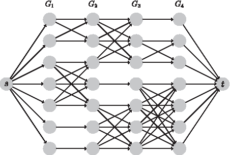
An example of the layered weighted bipartide matching problem. The nodes in this problem represent the nodes in the respective graphs and the edges represent the similarities that have been calculated with the weights being the similarity scores. In cases where the number of candidate nodes in each network is not the same, virtual “blank” nodes are added. This also allows for a network to be completely skipped by the alignment algorithm if it is drastically different from all other networks.

A potential limitation of this approach is that input order influences the accuracy of the alignment. We have experimentally discovered that while there is a variation in accuracy, there is no strong pattern as to the ordering of input networks (Fig. 1). While this is not an ideal situation, our approach allows for alignment of many networks and still compares favorably with current methods, and given the relatively low computational requirements of our approach, it is possible to perform sampling of input ordering and calculate several multiple alignments before other approaches can complete a single alignment. This is especially true for large sets of networks (see Results).

FIG. 1.

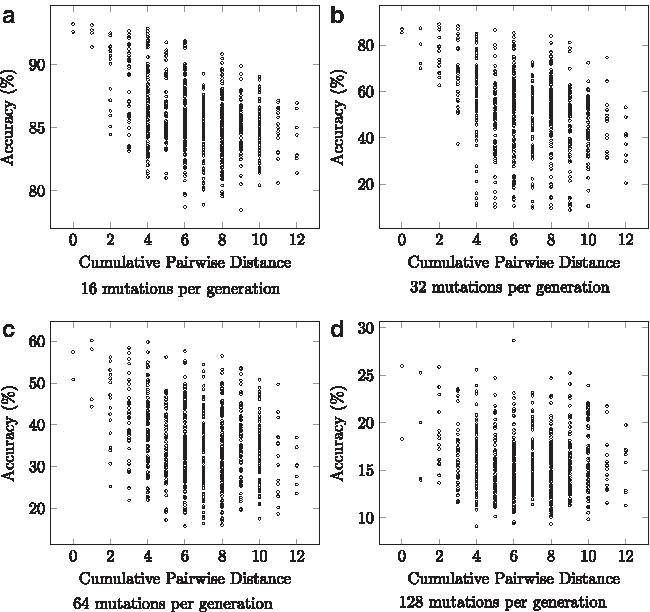
Accuracy variation based on network ordering. To observe the variation in accuracy based on input ordering, we aligned a set of networks with increasing differences in all possible ordering permutations. These different networks were created by mutating networks with a given number of mutations. The mutations performed on the networks were node addition/deletion, and edge addition/deletion with each node or edge, and the choice of addition or deletion selected at uniform random. While there is a difference in alignment accuracy as the input order varies, there is no clearly discernible pattern, especially as the difference between network increases.

2.1. Measures of accuracy

Our network alignment accuracy metrics use a parameterized accuracy function to calculate the proportion of edges that are conserved across a given number of networks. This generates an accuracy “curve” that we believe is superior to a single numerical representation, as it is able to provide a more granular portrayal of the similarity between multiple networks.

The “fair assessment” of many-to-many alignments posed a challenge, but we believe that our approach has resolved this satisfactorily. We deal with these alignments through the use of “expected” edges. That is, if there is an observed edge between node u and node x in network A, and the mapping has defined node x and node y as structurally indistinguishable in network A, then there should also be an edge between u and y in A. If this “expected” edge does not exist, then we define this edge as induced but not observed and define it as an edge conserved across zero networks. In this manner, many-to-many alignments are penalized only in cases where the ambiguity in the mapping will generate multiple induced edges that are not observed, and are given a better score in comparison to one-to-one mappings in cases where there is no ambiguity and the set of vertices is truly homologous.

We present induced multiple edge correctness (IMEC) as the accuracy metric devised for multiple network alignment. IMEC is a curve made up of a number of parameterized IMEC_m scores, where 1 ≤ m ≤ k and k is the number of networks being aligned.

Consider k networks \documentclass{aastex}\usepackage{amsbsy}\usepackage{amsfonts}\usepackage{amssymb}\usepackage{bm}\usepackage{mathrsfs}\usepackage{pifont}\usepackage{stmaryrd}\usepackage{textcomp}\usepackage{portland, xspace}\usepackage{amsmath, amsxtra}\pagestyle{empty}\DeclareMathSizes {10} {9} {7} {6} \begin{document} $$G_1 = ( V_1 , E_1 ) , \ldots , G_k = ( V_k , E_k )$$ \end{document} . The alignment is a mapping f : {ν_i} where ν_i is a tuple of subsets of \documentclass{aastex}\usepackage{amsbsy}\usepackage{amsfonts}\usepackage{amssymb}\usepackage{bm}\usepackage{mathrsfs}\usepackage{pifont}\usepackage{stmaryrd}\usepackage{textcomp}\usepackage{portland, xspace}\usepackage{amsmath, amsxtra}\pagestyle{empty}\DeclareMathSizes {10} {9} {7} {6} \begin{document} $$V_1 , \ldots , V_k$$ \end{document} such that \documentclass{aastex}\usepackage{amsbsy}\usepackage{amsfonts}\usepackage{amssymb}\usepackage{bm}\usepackage{mathrsfs}\usepackage{pifont}\usepackage{stmaryrd}\usepackage{textcomp}\usepackage{portland, xspace}\usepackage{amsmath, amsxtra}\pagestyle{empty}\DeclareMathSizes {10} {9} {7} {6} \begin{document} $$\nu_i = ( W_{1 , i} , \ldots , W_{k , i} )$$ \end{document} where W_m_,i is a subset of V_m in the i^th tuple of f. W_m,i ∩ W_m_,j = ∅ ∀ i ≠ j, that is, no vertex appears in more than one subset. This permits W_m_,j = ∅ and does not require that \documentclass{aastex}\usepackage{amsbsy}\usepackage{amsfonts}\usepackage{amssymb}\usepackage{bm}\usepackage{mathrsfs}\usepackage{pifont}\usepackage{stmaryrd}\usepackage{textcomp}\usepackage{portland, xspace}\usepackage{amsmath, amsxtra}\pagestyle{empty}\DeclareMathSizes {10} {9} {7} {6} \begin{document} $$\bigcup \limits_{i}W_{m , i} = V_m$$ \end{document} , that is, not every node need be mapped.

Let S(f) be a network (V*, E*) where V* = {ν_i}, that is, f determines V* directly and S(f) represents the alignment. E* is such that \documentclass{aastex}\usepackage{amsbsy}\usepackage{amsfonts}\usepackage{amssymb}\usepackage{bm}\usepackage{mathrsfs}\usepackage{pifont}\usepackage{stmaryrd}\usepackage{textcomp}\usepackage{portland, xspace}\usepackage{amsmath, amsxtra}\pagestyle{empty}\DeclareMathSizes {10} {9} {7} {6} \begin{document} $$e \in E^* \ { \rm iff} \ \exists \ i , j , m : v \in W_{m , i} , w \in W_{m , j} , ( v , w ) \in E_k$$ \end{document} ; that is, E* is the set of edges that appear in at least one network and have both end nodes in the mapping. This allows i = j for self loops. The function \documentclass{aastex}\usepackage{amsbsy}\usepackage{amsfonts}\usepackage{amssymb}\usepackage{bm}\usepackage{mathrsfs}\usepackage{pifont}\usepackage{stmaryrd}\usepackage{textcomp}\usepackage{portland, xspace}\usepackage{amsmath, amsxtra}\pagestyle{empty}\DeclareMathSizes {10} {9} {7} {6} \begin{document} $$weight( e \in E^* ) = max$$ \end{document} (1, number of networks containing e).

Let \documentclass{aastex}\usepackage{amsbsy}\usepackage{amsfonts}\usepackage{amssymb}\usepackage{bm}\usepackage{mathrsfs}\usepackage{pifont}\usepackage{stmaryrd}\usepackage{textcomp}\usepackage{portland, xspace}\usepackage{amsmath, amsxtra}\pagestyle{empty}\DeclareMathSizes {10} {9} {7} {6} \begin{document} $$E^*_m = \{ e \in E^* \mid weight ( e ) \geq m \} $$ \end{document} . IMEC _m is given by: \documentclass{aastex}\usepackage{amsbsy}\usepackage{amsfonts}\usepackage{amssymb}\usepackage{bm}\usepackage{mathrsfs}\usepackage{pifont}\usepackage{stmaryrd}\usepackage{textcomp}\usepackage{portland,xspace}\usepackage{amsmath,amsxtra}\pagestyle{empty}\DeclareMathSizes{10}{9}{7}{6} \begin{document} \begin{align*} { \rm IMEC } _m ( f ) = \frac { \sum \limits_ { e \in E_m^* } { weight ( e ) } } { \sum \limits_ { a \in E^* } { weight ( a ) } } \tag { 1 } \end{align*} \end{document}

A variant of this score curve, the comprehensive multiple edge correctness (CMEC) score, was also devised to include edges that are not in the generated alignment network defined above, but exist in the input networks. The calculation steps of the score are identical to the calculation of IMEC, but the divisor for the CMEC_m score includes the number of edges that are in the input networks but are not included in the alignment network.

Let \documentclass{aastex}\usepackage{amsbsy}\usepackage{amsfonts}\usepackage{amssymb}\usepackage{bm}\usepackage{mathrsfs}\usepackage{pifont}\usepackage{stmaryrd}\usepackage{textcomp}\usepackage{portland, xspace}\usepackage{amsmath, amsxtra}\pagestyle{empty}\DeclareMathSizes {10} {9} {7} {6} \begin{document} $$E^{ \prime}_k = \{ e \mid e \,\notin\, E^* , e \in E_k \} $$ \end{document} . CMEC_m is given by: \documentclass{aastex}\usepackage{amsbsy}\usepackage{amsfonts}\usepackage{amssymb}\usepackage{bm}\usepackage{mathrsfs}\usepackage{pifont}\usepackage{stmaryrd}\usepackage{textcomp}\usepackage{portland,xspace}\usepackage{amsmath,amsxtra}\pagestyle{empty}\DeclareMathSizes{10}{9}{7}{6} \begin{document} \begin{align*} { \rm CMEC } _m ( f ) = \frac { \sum \limits_ { e \in E^*_m } { weight ( e ) } } { \sum \limits_ { a \in E^* } { weight ( a ) } + \sum \limits_ { k } \mid E^ { \prime } _k \mid } \tag { 2 } \end{align*} \end{document}

3. Methods

3.1. Experimental procedure

The experiments were originally performed on a standard desktop machine with four physical cores running at 3.4 GHz and 8 GB of RAM. We discovered that some algorithms required more RAM than was available on this machine, so we performed these experiments on a server class machine with 32 physical cores at 2 GHz and 512 GB of RAM to ensure memory requirements were adequately satisfied. However, these experiments took over 72 hours and were aborted, with some algorithms exhibiting a memory requirement exceeding 200 GB of RAM. All results presented are from executions on the standard desktop machine.

Experiments one (E1-HuEtal1), two (E2-HuEtal2), and three (E3-HuEtal3) are a replication of the experiments performed by Hu et al. (2014). With these experiments we wished to compare the accuracy of existing algorithms on an already analyzed dataset. Experiment four (E4-HerpesVirus) is the alignment of four highly similar, small networks. We expected the accuracy to be high and the resource requirements low for all algorithms on this dataset. We devised experiment five (E5-Stress) as a “stress” test for the alignment algorithms. In this experiment there is little similarity between the organisms being compared; network sizes vary greatly, and there are a large number of networks, aggregating into a challenging alignment situation. We expected the accuracy to be low and the resource requirements very high for this experiment. Experiment six (E6-Large) contains only networks with more than 2500 unique proteins. The organisms are distantly related, but the variation in network sizes is less than with other experiments. We expected that the accuracy will be higher than experiment five, but still remain low. Experiment seven (E7-Mammals) contains only mammals, and as such we expected that the accuracy will be relatively high. The variation in network sizes is a clear indication that the accuracy may not be as high as we might expect with more balanced network sizes.

The ordering of inputs for NH was done arbitrarily (alphabetically) for all experiments. We did not perform a range of alignments with different orderings to choose the most accurate, however, in general, we have found that the ordering does not make a big difference (Fig. 1).

3.2. Data

The protein–protein interaction networks were obtained from the supplementary material of the NetCoffee publication (Hu et al., 2014), and inferred from the protein–protein interaction data from BioGRID (accessed June 2014). The networks derived from the interaction data from BioGRID contain only unique proteins and unique interactions. We accepted all forms of experimental evidence of a protein–protein interaction in this dataset. Network statistics as well as experiment participation are given in Table 1.

Table 1.

A List of Data Sources, Organisms, Network Properties, and the Networks Compared in the Experiments Performed

Source	Organism	Unique proteins	Unique interactions	Experiment
NetCoffee	Homo sapiens	8777	28366	—	—	3	—	—	—	—
NetCoffee	Mus musculus	1531	1626	—	2	3	—	—	—	—
NetCoffee	Drosophila melanogaster	1534	2664	1	2	3	—	—	—	—
NetCoffee	Caenorhabditis elegans	767	915	1	2	3	—	—	—	—
NetCoffee	Saccharomyces cerevisiae	5739	36226	1	2	3	—	—	—	—
BioGRID	Bos taurus	351	311	—	—	—	—	5	—	7
BioGRID	Caenorhabditis elegans	3898	7921	—	—	—	—	5	6	—
BioGRID	Danio rerio	229	245	—	—	—	—	5	—	—
BioGRID	Drosophila melanogaster	8224	39252	—	—	—	—	5	6	—
BioGRID	Gallus gallus	322	332	—	—	—	—	5	—	—
BioGRID	Homo sapiens	18629	149703	—	—	—	—	5	6	7
BioGRID	Human herpesvirus 1	137	137	—	—	—	4	—	—	—
BioGRID	Human herpesvirus 4	219	217	—	—	—	4	—	—	—
BioGRID	Human herpesvirus 5	69	60	—	—	—	4	—	—	—
BioGRID	Human herpesvirus 8	132	130	—	—	—	4	—	—	—
BioGRID	Mus musculus	8293	18620	—	—	—	—	5	6	7
BioGRID	Oryctolagus cuniculus	145	135	—	—	—	—	5	—	7
BioGRID	Rattus norvegicus	2794	3790	—	—	—	—	5	6	7
BioGRID	Xenopus laevis	467	518	—	—	—	—	5	—	—

The networks belonging to the NetCoffee dataset are not guaranteed to have unique interactions, whereas the networks derived from BioGRID have unique interactions.

4. Results

We discovered that NH compares favorably in terms of accuracy, runtime, and memory requirements with current algorithms. From Table 2, we note that while NH is not the fastest or the most memory efficient approach in experiments E1-HuEtal1, E2-HuEtal2, or E3-HuEtal3, which use the NetCoffee dataset (Hu et al., 2014), it does exhibit substantially better EC, ICS, and S³ scores. The runtime and memory requirements are still within a respectable bound of the fastest and most lightweight algorithms for these experiments. From Figure 3, it is clear that NH has the shallowest IMEC and CMEC curve, indicating a more accurate global alignment.

FIG. 3.

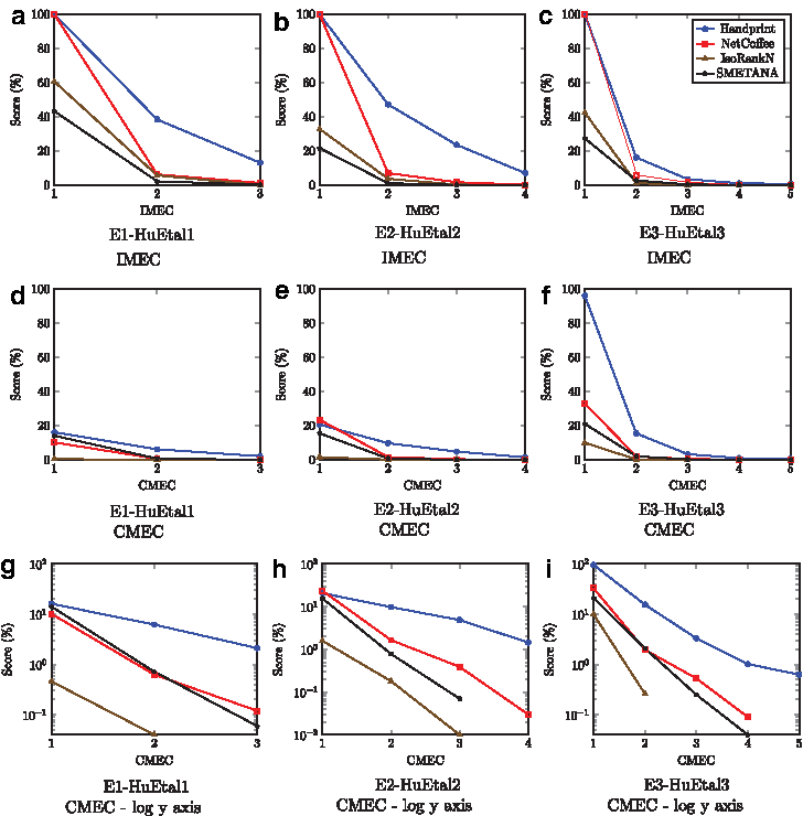
Comparison of existing algorithms: NetCoffee dataset and experiments using IMEC and CMEC curves. (a–c) IMEC curve across the three NetCoffee-based experiments. (d and e) CMEC curve across the three NetCoffee-based experiments. (g and h) CMEC curve across the three NetCoffee-based experiments using a logarithmic y axis to display the rate of accuracy loss. The IMEC curves are very steep across all network alignments and all datasets. This indicates that the networks being compared have little similarity between them. This is as expected since both the organisms and network sizes are highly disparate. This is further exhibited by the CMEC curve, as CMEC-1 is low for E1-HuEtal1 and E2-HuEtal2. NH performs better than the other alignment algorithms on this dataset for all points except CMEC-1 for E2-HuEtal2. CMEC, comprehensive multiple edge correctness; IMEC, induced multiple edge correctness; NH, node handprinting.

Table 2.

Performance Comparison of Existing Algorithms

Experiment	Metric	NH	NetCoffee	IsoRankN	SMETANA
E1-HuEtal1	Runtime	1 m 30.45 s	1.63 s	1 h 45 m 3 s	29.3 s
	Memory	84.97 MB	26.16 MB	563.34 MB	257.46 MB
	EC	21.84%	1.27%	0%	0.74%
	ICS	12.16%	0.67%	0%	0.19%
	S ³	8.47%	0.44%	0%	0.15%
E2-HuEtal2	Runtime	1 m 19.21 s	18.17 s	2 h 17 m 17 s	2 m 1.32 s
	Memory	172.7 MB	95.5 MB	730.63 MB	381.71 MB
	EC	11.11%	0.27%	0%	0%
	ICS	10.59%	0.07%	0%	0%
	S ³	5.73%	0.06%	0%	0%
E3-HuEtal3	Runtime	7 m 51.85 s	39.4 s	10 h 12 m 12 s	3 m 34.91 s
	Memory	486.18 MB	133.54 MB	1479.19 MB	577.26
	EC	7.37%	0%	0%	0.13%
	ICS	0.27%	0%	0%	0.01%
	S ³	0.26%	0%	0%	0%
E4-HerpesVirus	Runtime	0.12 s	1.04 s	11.74 s	55.5 s
	Memory	9.4 MB	9.94 MB	33.3 MB	231.175 MB
	EC	33.33%	0%	0%	6.67%
	ICS	12.82%	0%	0%	2.5%
	S ³	10.2%	0%	0%	1.85%
E5-Stress	Runtime	9 h 59 m 14 s	>72 h	>72 h	>72 h
	Memory	2.8 GB	>200 GB	>512 GB	>200 GB
	EC	3.76%	—	—	—
	ICS	<0.01 %	—	—	—
	S ³	<0.01 %	—	—	—
E6-Large	Runtime	4 h 52 m 32 s	>72 h	>72 h	>72 h
	Memory	1.9 GB	>200 GB	>512 GB	>200 GB
	EC	2.28%	—	—	—
	ICS	0.18%	—	—	—
	S ³	0.16%	—	—	—
E7-Mammals	Runtime	8 h 37 m 5 s	>72 h	>72 h	>72 h
	Memory	2.2 GB	>200 GB	>512 GB	>200 GB
	EC	6.39%	—	—	—
	ICS	0.06%	—	—	—
	S ³	0.06%	—	—	—

We note that while NH is not always the fastest alignment algorithm, it is able to calculate a much better alignment using reasonable computational resources. NH is also the only algorithm that is capable of handling the BioGRID dataset within a reasonable amount of time. NH was able to complete all alignments using the moderate resources of a standard desktop machine and does not require specialized hardware to perform the alignments.

E4-HerpesVirus is the only experiment using the BioGRID (Stark et al., 2006) dataset that all alignment algorithms completed within 72 hours. With this dataset we see NH being quicker and more memory efficient than the other alignment algorithms. Using EC, ICS, and S³, NH is far more accurate, with only SMETANA of the remaining methods able to calculate an alignment with a score above 0%. With E5-Stress, E6-Large, E7-Mammals, NH is the only alignment algorithm that is able to complete the alignment within 72 hr. Other alignment algorithms also required copious amounts of RAM (see Table 2), whereas NH could compute the alignment on a modest desktop machine. Over these experiments, we note that EC, ICS, and S³ are extremely low, especially ICS and S³. From these values, along with the IMEC and CMEC curves shown in Figure 4, we deduce that these networks have very different structures. We do note that the alignments of closely related organisms such as those in E4-HerpesVirus and E7-Mammals have shallower curves than experiments that include distantly related organisms. We believe that the reason E7-Mammals exhibits curve features that would be more in line with an alignment of distantly related organisms is that the sizes of the networks being compared are so dissimilar. We expect the accuracy to improve, and more common features to be discovered as more interactions are measured in the nonhuman mammals.

FIG. 4.

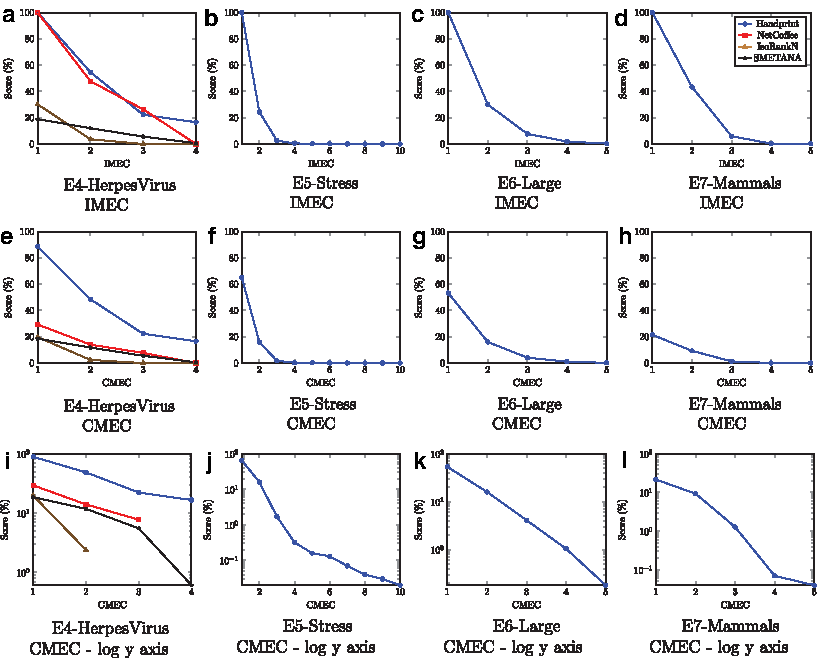
Alignment of the networks from BioGrid. (a–d) IMEC curve across the four BioGRID-based experiments. (e–h) CMEC curve across the four BioGRID experiments. (i–l) CMEC curve across the four BioGRID experiments using a logarithmic y axis. Only NH was able to complete the alignment for the larger experiments in this dataset. We noted that IMEC and CMEC curves are shallower when comparing closely related organisms than those with similar sizes. We believe that the sharp drop in IMEC for E7-Mammals is because of the disparity of network sizes of the mammals being compared.

5. Discussion

5.1. Accuracy

We compared the alignments using both modified metrics from pairwise alignment and our new metrics. While the classic measures of accuracy, extended into the multiple alignment space, are still capable of providing a notion of the similarity of the networks being aligned, they do not provide the depth of information that IMEC and CMEC are able to. NH is able to perform very competitively with state-of-the art algorithms, even with the variance of accuracy based on input ordering. We would also like to note that it is possible to apply sampling to the order of inputs and get multiple alignments out of NH before any of the other algorithms are able to finish one alignment in some experiments. We also present a simple visualization in Figure 5 of the alignment resulting from E4-HerpesVirus by both NH and NetCoffee to compare the difference in accuracy visually. We selected the resulting alignment for this experiment largely by the size of the input networks. Current visualization techniques do not scale well with large networks in terms of both runtime and usability. We did not visualize the alignment given by IsoRankN and SMETANA because our visualization solution was unable to handle many-to-many alignments gracefully.

FIG. 5.

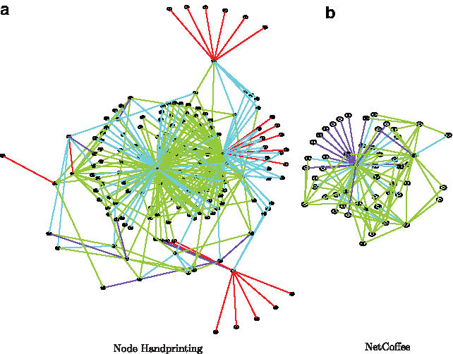
Visualization of the alignment of E4-HerpesVirus using (a) NH and (b) NetCoffee. Cooler colored edges (e.g., green and blue) denote that the edge has been conserved across fewer networks, and warmer colored edges (e.g., purple and red) express highly conserved edges. The visualization was performed only with NH and NetCoffee since these algorithms were the most accurate on this dataset, as well as the inability of this visualization approach to handle many-to-many mappings. The node labels represent the lines of the alignment (and therefore the protein interactions aligned as homologous by the algorithms). NH not only aligns a greater proportion of the proteins, but it is capable of aligning several fan structures that are common across all networks, whereas NetCoffee does not.

5.2. Computation time

While NH is not the fastest algorithm compared across all experiments, it was always within a reasonable margin of the fastest method. NH was the only alignment algorithm that is capable of performing the strenuous experiments.

A tight upper bound of the time complexity of the algorithm remains an open problem as it depends on the structure, density, similarity of the networks being compared, as well as the uniqueness of the structures within each network. We offer an approximation of the computational complexity but stress that this is very rough.

We consider k networks \documentclass{aastex}\usepackage{amsbsy}\usepackage{amsfonts}\usepackage{amssymb}\usepackage{bm}\usepackage{mathrsfs}\usepackage{pifont}\usepackage{stmaryrd}\usepackage{textcomp}\usepackage{portland, xspace}\usepackage{amsmath, amsxtra}\pagestyle{empty}\DeclareMathSizes {10} {9} {7} {6} \begin{document} $$G_1 = ( V_1 , E_1 ) \ldots G_k = ( V_k , E_k )$$ \end{document} as before. Let the average number of nodes be defined as \documentclass{aastex}\usepackage{amsbsy}\usepackage{amsfonts}\usepackage{amssymb}\usepackage{bm}\usepackage{mathrsfs}\usepackage{pifont}\usepackage{stmaryrd}\usepackage{textcomp}\usepackage{portland, xspace}\usepackage{amsmath, amsxtra}\pagestyle{empty}\DeclareMathSizes {10} {9} {7} {6} \begin{document} $$n = ( \mid V_1 \mid + \ldots + \mid V_k \mid ) / k$$ \end{document} and the average degree of nodes in \documentclass{aastex}\usepackage{amsbsy}\usepackage{amsfonts}\usepackage{amssymb}\usepackage{bm}\usepackage{mathrsfs}\usepackage{pifont}\usepackage{stmaryrd}\usepackage{textcomp}\usepackage{portland, xspace}\usepackage{amsmath, amsxtra}\pagestyle{empty}\DeclareMathSizes {10} {9} {7} {6} \begin{document} $$V_1 \ldots V_k$$ \end{document} be ρ where 0 < ρ ≤ n. To calculate the score function s(x, y), all adjacent nodes must be visited once for each candidate node, resulting in an average runtime equal to the average density squared (ρ²), resulting in a worst case O(n²). Biological networks are generally sparse, and in our experience have a very small average node density, so ρ will be significantly smaller than n. The score function is executed for all candidate pairings. There are ρn candidate pairings for each adjacent network pair since the n nodes in one graph must be compared to ρ nodes from the other. This is repeated across (k−1) adjacent network pairings. Thus the rough approximation of the computational complexity of this step is equal to ρ³n(k−1) with a worst case complexity of O(n⁴k).

Once the nodes are scored, we use a layered weighted bipartide matching solver to combine these pairwise “fragments” into a multiple alignment. In our initial implementation, this step has a complexity of ρn²k². This gives the program an overall complexity of ρ³nk + ρn²k², with a worst case O(n³k(n + k)). We performed several experiments to validate our rough complexity approximation, the results of which are shown in Figures 6 and 7.

FIG. 6.

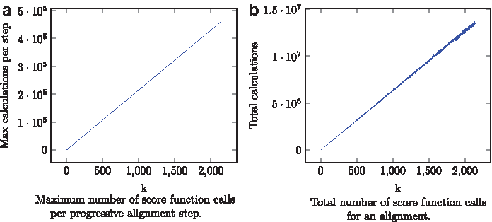
Resource usage scaling with varying the number of networks aligned (k). (a) and (b) represent the alignment of k distinctly generated networks with 400 nodes each. These networks were generated by GNLab. Each point is the average of 10 executions, each sampling a different input order. We found very little difference in both runtime and RAM usage between the different input orderings. (c) and (d) show the alignment of k identical networks. These networks were generated by GNLab and have 100 vertices. Both of these plots show a distinct quadratic curve.

FIG. 7.

Number of score function calls that must be performed with varying k. (a) The maximum number of score function calls that must be performed during an alignment. (b) The total number of score function calls that must be executed during an alignment. These results are using the same dataset as Figure 6c and d.

5.3. Memory requirements

The memory requirements of NH are not the lowest in all experiments performed, but were always within a reasonable margin of the most memory efficient alignment algorithm. NH has the best memory scaling however, and is the only alignment algorithm that is able to run on a standard desktop machine while allowing a realistic number of large networks to be aligned. While aligning networks from BioGRID dataset, NH requires less memory than other alignment algorithms. We believe that, as with runtime, the memory requirement of NH is highly dependent on the structure of networks being compared.

6. Conclusion

We have presented NH, a fast, accurate, lightweight, and highly scalable method for global alignment of multiple biological networks. We have compared our method to current multiple network alignment approaches and have found that NH is able to compute alignments with a favourable accuracy while using reasonable computational resources. It is also the only algorithm that is capable of aligning the larger networks from BioGrid. While NH is not guaranteed to give an optimal alignment, and the alignment quality may vary based on input ordering, it does provide a good alignment using minimal computational resources.

Footnotes

Acknowledgment

Funding: This work was supported by the Australian Postgraduate Award to A. Radu.

Author Disclosure Statement

The authors declare that no competing financial interests exist.

References

Aladag

A.E.

, and Erten

2013. SPINAL: scalable protein interaction network alignment. Bioinformatics, 29, 917–924.

El-Kebir

, Heringa

, and Klau

2011. Lagrangian relaxation applied to sparse global network alignment. Pattern Recognit. Bioinform., 7036, 225–236.

Flannick

, Novak

, Srinivasan

B.S.

, et al. 2006. Graemlin: general and robust alignment of multiple large interaction networks. Genome Res., 16, 1169–1181.

, Kehr

, and Reinert

2014. NetCoffee: a fast and accurate global alignment approach to identify functionally conserved proteins in multiple networks. Bioinformatics, 30, 540–548.

Kalaev

, Smoot

, Ideker

, and Sharan

2008. NetworkBLAST: comparative analysis of protein networks. Bioinformatics, 24, 594–596.

Kelley

B.P.

, Yuan

, Lewitter

, et al. 2004. PathBLAST: 20 a tool for alignment of protein interaction networks. Nucleic Acids Res., 32, W83–W88.

Koyutürk

, Kim

, Topkara

, et al. 2006. Pairwise alignment of protein interaction networks. J. Comput. Biol., 13, 182–199.

Kuchaiev

, Milenkovic

, Memisevic

, et al. 2010. Topological network alignment uncovers biological function and phylogeny. J. R. Soc. Interface, 7, 1341–1354.

Milo

, Shen-Orr

, Itzkovitz

, et al. 2002. Network motifs: simple building blocks of complex networks. Science, 298, 824.

10.

Pache

, Céol

, and Aloy

2012. NetAligner—a network alignment server to compare complexes, pathways and whole interactomes. Nucleic Acids Res., 40, W157–W161.

11.

Patro

, and Kingsford

2012. Global network alignment using multiscale spectral signatures. Bioinformatics, 28, 3105–3114.

12.

Phan

H.T.T.

, and Sternberg

M.J.E.

2012. PINALOG: a novel approach to align protein interaction networks—implications for complex detection and function prediction. Bioinformatics, 28, 1239–1245.

13.

Radu

, and Charleston

2014. Node fingerprinting: an efficient heuristic for aligning biological networks. J. Comput. Biol., 21, 760–770.

14.

Sahraeian

S.M.E.

, and Yoon

B.-J.

2013. SMETANA: accurate and scalable algorithm for probabilistic alignment of large-scale biological networks. PloS One, 8, e67995.

15.

Saraph

, and Milenković

2013. MAGNA: Maximizing Accuracy in Global Network Alignment. Bioinformatics, 30, 2931–2940.

16.

Singh

, Xu

, and Berger

2007. Pairwise global alignment of protein interaction networks by matching neighborhood topology. Res. Comput. Mol. Biol. 16–31.

17.

Singh

, Xu

, and Berger

2008. Global alignment of multiple protein interaction networks with application to functional orthology detection. Proc. Natl. Acad. Sci. USA, 105, 12763–12768.

18.

Stark

, Breitkreutz

B.-J.

, Reguly

, et al. 2006. BioGRID: a general repository for interaction datasets. Nucleic Acids Res., 34, D535–D539.