A Nonhomogeneous Hidden Markov Model for Gene Mapping Based on Next-Generation Sequencing Data

Abstract

The analysis of polygenetic characteristics for mapping quantitative trait loci (QTL) remains an important challenge. QTL analysis requires two or more strains of organisms that differ substantially in the (poly-)genetic trait of interest, resulting in a heterozygous offspring. The offspring with the trait of interest is selected and subsequently screened for molecular markers such as single-nucleotide polymorphisms (SNPs) with next-generation sequencing. Gene mapping relies on the co-segregation between genes and/or markers. Genes and/or markers that are linked to a QTL influencing the trait will segregate more frequently with this locus. For each identified marker, observed mismatch frequencies between the reads of the offspring and the parental reference strains can be modeled by a multinomial distribution with the probabilities depending on the state of an underlying, unobserved Markov process. The states indicate whether the SNP is located in a (vicinity of a) QTL or not. Consequently, genomic loci associated with the QTL can be discovered by analyzing hidden states along the genome. The aforementioned hidden Markov model assumes that the identified SNPs are equally distributed along the chromosome and does not take the distance between neighboring SNPs into account. The distance between the neighboring SNPs could influence the chance of co-segregation between genes and markers. To address this issue, we propose a nonhomogeneous hidden Markov model with a transition matrix that depends on a set of distance-varying observed covariates. The application of the model is illustrated on the data from a study of ethanol tolerance in yeast.

1. Introduction

The analysis of polygenetic characteristics for mapping quantitative trait loci (QTL) has received a substantial amount of consideration in molecular genetics over the last decades. QTL analysis is a method that links two types of information—phenotypic data (trait measurements) and genotypic data (usually molecular markers)—in an attempt to interpret the genetic basis of variation in traits and to link certain phenotypes to specific regions of chromosomes. The goal of this process is to identify the precise location of these linked chromosomal regions across the genome by looking for evidence of co-segregation, that is, the tendency for closely linked genes and genetic markers to be inherited together.

QTL analysis requires two or more strains of organisms that differ substantially in the quantitative trait of interest and reliable scoring of genetic markers. For this purpose, a cross is obtained from two parental strains, creating the first generation of heterozygous offspring (F1). The offspring with the phenotype of interest is identified and screened for genetic markers, such as single-nucleotide polymorphisms (SNPs). The advent of high-throughput technologies such as next-generation sequencing (NGS) (Shendure and Ji, 2005) provides a new way to score large numbers of genetic markers. Markers that are linked to a QTL influencing the trait of interest have a tendency to be inherited more frequently with this locus, whereas unlinked markers will not show any substantial association with the phenotype of interest.

Recently, a hidden Markov model (HMM) was proposed by Claesen and Burzykowski (2014) to map QTLs using NGS-assisted bulked segregant analysis (BSA) (Schneeberger et al., 2009). HMMs (MacDonald and Zucchini, 1997) consist of two stochastic processes: a (hidden) sequence of states characterized by the state transition probability distribution with a Markov chain property and a sequence of observations with state-dependent probability distribution. The HMM proposed by Claesen and Burzykowski (2014) provides a flexible approach to classify each identified SNP into one of several predefined states, which have their own specific biological interpretation. The identified states of the HMM allow to identify genomic regions that may be likely to contain trait-related genes.

The model proposed by Claesen and Burzykowski (2014) assumes that the identified SNPs are equally spaced across the whole genome. This assumption is not necessarily correct. On the other hand, the chance of co-segregation may depend on the distance between the SNPs. Hence, an extension of the HMM that accommodates the distance between SNPs is of interest. Toward this aim, the assumption that the latent Markov chain is homogeneous, that is, that the transition probabilities are constant, can be weakened. More specifically, the transition probabilities can be assumed to depend on the distance between SNPs. This results in a nonhomogeneous HMM (NH-HMM) model. Such models have been considered, for example, in environmental studies (Zucchini and Guttorp, 1991; Hughes and Guttorp, 1994; Charles et al., 1999; Hughes et al., 1999; Bellone et al., 2000; Charles et al., 2004; Robertson et al., 2004; Betrò et al., 2008). In our article, we apply an NH-HMM to the analysis of an experiment aimed at finding QTLs for high ethanol tolerance in Saccharomyces cerevisiae.

2. Data

In the case study, BSA (Schneeberger et al., 2009) was combined with NGS to allow simultaneous identification of many genetic markers.

A highly ethanol-tolerant yeast strain (S. cerevisiae) was crossed with a laboratory strain (without the trait) of a moderate ethanol tolerance, resulting in 5974 viable haploid yeast cells (Swinnen et al., 2012a,b). Haploid offspring was screened for high ethanol tolerance, first in a medium containing 16% of ethanol producing 136 ethanol-tolerant segregants and subsequently with 17% ethanol giving rise to 31 segregants. The genomic DNA from both pools, 16% ethanol (pool 1) and 17% ethanol (pool 2), and the parent strains with high ethanol tolerance was submitted to a pooled-segregant genome-wide sequencing analysis by means of high-throughput NGS using the Illumina/Solexa technique. The technique produced DNA sequences. These reads were subsequently aligned to a DNA sequence of the parental laboratory yeast strain (without the trait) and SNPs as genetic markers were identified. For each identified SNP, the chromosomal position, the number of sequencing events (reads), and the number of times that the nucleotides A, C, G, and T were present in the offspring were recorded. The larger the proportion of differences in terms of the nucleotides (mismatch/SNP frequency) between the offspring and the parental strain, the higher the chance of a presence of a trait-related gene in the vicinity of the chromosomal location.

3. Methodology

3.1. A homogeneous HMM

HMMs are a particular kind of mixture models that allow for serially dependent observations. An HMM consists of two components. The first component is a “parameter process” (Zucchini and MacDonald, 2009). It is a sequence \documentclass{aastex}\usepackage{amsbsy}\usepackage{amsfonts}\usepackage{amssymb}\usepackage{bm}\usepackage{mathrsfs}\usepackage{pifont}\usepackage{stmaryrd}\usepackage{textcomp}\usepackage{portland, xspace}\usepackage{amsmath, amsxtra}\pagestyle{empty}\DeclareMathSizes{10}{9}{7}{6}\begin{document} $$\{C_1 , C_2 , \ldots \}$$ \end{document} of discrete random variables that can assume one of m possible values (“states”) from a set \documentclass{aastex}\usepackage{amsbsy}\usepackage{amsfonts}\usepackage{amssymb}\usepackage{bm}\usepackage{mathrsfs}\usepackage{pifont}\usepackage{stmaryrd}\usepackage{textcomp}\usepackage{portland, xspace}\usepackage{amsmath, amsxtra}\pagestyle{empty}\DeclareMathSizes{10}{9}{7}{6}\begin{document} $$\Sigma = \{s_1 , s_2 , \ldots , s_m \} $$ \end{document} . We assume that the sequence of states forms a first-order Markov chain; that is, \documentclass{aastex}\usepackage{amsbsy}\usepackage{amsfonts}\usepackage{amssymb}\usepackage{bm}\usepackage{mathrsfs}\usepackage{pifont}\usepackage{stmaryrd}\usepackage{textcomp}\usepackage{portland, xspace}\usepackage{amsmath, amsxtra}\pagestyle{empty}\DeclareMathSizes{10}{9}{7}{6}\begin{document} $${\rm P} ( C_i \mid C_1 , \ldots , C_{i - 1} ) = {\rm P} ( C_i \mid C_{i - 1} )$$ \end{document} . Moreover, we assume that, for all i, P(C_i = s_j | C_i−₁ = s_k) ≡ γ_jk, where γ_jk is the probability of transition from state s_j to state s_k. The transition probabilities form the state-transition probability matrix Γ , with the element in jth row and kth column equal to γ_jk. Additionally, we specify the “initial state” probability distribution; that is, P(C₁ = s_j) ≡ δ_j, say.

The second part of an HMM is a “state-dependent” process \documentclass{aastex}\usepackage{amsbsy}\usepackage{amsfonts}\usepackage{amssymb}\usepackage{bm}\usepackage{mathrsfs}\usepackage{pifont}\usepackage{stmaryrd}\usepackage{textcomp}\usepackage{portland, xspace}\usepackage{amsmath, amsxtra}\pagestyle{empty}\DeclareMathSizes{10}{9}{7}{6}\begin{document} $$\{X_{1} , X_{2} , \ldots \} $$ \end{document} . The distribution of random variable X_i depends on state C_i; that is, \documentclass{aastex}\usepackage{amsbsy}\usepackage{amsfonts}\usepackage{amssymb}\usepackage{bm}\usepackage{mathrsfs}\usepackage{pifont}\usepackage{stmaryrd}\usepackage{textcomp}\usepackage{portland, xspace}\usepackage{amsmath, amsxtra}\pagestyle{empty}\DeclareMathSizes{10}{9}{7}{6}\begin{document} $${\rm P} ( X_i \mid X_1 , \ldots , X_{i - 1} , C_1 , \ldots , C_i ) = {\rm P} ( X_i \, \mid \, C_i )$$ \end{document} . In particular, we assume that P(X_i = x | C_i = s_j), the “emission probability” of x for state s_j, depends on a vector of parameters θ _j. We define \documentclass{aastex}\usepackage{amsbsy}\usepackage{amsfonts}\usepackage{amssymb}\usepackage{bm}\usepackage{mathrsfs}\usepackage{pifont}\usepackage{stmaryrd}\usepackage{textcomp}\usepackage{portland, xspace}\usepackage{amsmath, amsxtra}\pagestyle{empty}\DeclareMathSizes{10}{9}{7}{6}\begin{document} $${\boldsymbol{\theta}} = ( {\boldsymbol{\theta}}_1. \ldots , {\boldsymbol{\theta}}_\textbf{\textit{m}} )$$ \end{document} .

In practice, we observe only a sequence of values \documentclass{aastex}\usepackage{amsbsy}\usepackage{amsfonts}\usepackage{amssymb}\usepackage{bm}\usepackage{mathrsfs}\usepackage{pifont}\usepackage{stmaryrd}\usepackage{textcomp}\usepackage{portland, xspace}\usepackage{amsmath, amsxtra}\pagestyle{empty}\DeclareMathSizes{10}{9}{7}{6}\begin{document} $$\{X_1 = x_1 , X_2 = x_2 , \ldots , X_N = x_N \} $$ \end{document} , without the corresponding sequence of the generating states \documentclass{aastex}\usepackage{amsbsy}\usepackage{amsfonts}\usepackage{amssymb}\usepackage{bm}\usepackage{mathrsfs}\usepackage{pifont}\usepackage{stmaryrd}\usepackage{textcomp}\usepackage{portland, xspace}\usepackage{amsmath, amsxtra}\pagestyle{empty}\DeclareMathSizes{10}{9}{7}{6}\begin{document} $$\{C_1 = c_1 , C_2 = c_2 , \ldots , C_N = c_N \} $$ \end{document} . In other words, the Markovian “parameter process” is hidden from the observer and hence the name of the model.

Figure 1 schematically presents the HMM described above.

FIG. 1.

A HMM underlying the sequence of data values \documentclass{aastex}\usepackage{amsbsy}\usepackage{amsfonts}\usepackage{amssymb}\usepackage{bm}\usepackage{mathrsfs}\usepackage{pifont}\usepackage{stmaryrd}\usepackage{textcomp}\usepackage{portland, xspace}\usepackage{amsmath, amsxtra}\pagestyle{empty}\DeclareMathSizes{10}{9}{7}{6}\begin{document} $$( X_1 , \ldots , X_{i - 1} , X_i , X_{i + 1} , \ldots , X_N )$$ \end{document} . C_i is the hidden state for the observation X_i, P(X_i |C_i ) is the probability of emission of X_i in state C_i, and P(C_i|C_i₋₁) is the probability of transition from state C_i₋₁ to state C_i. HMM, hidden Markov model.

If the state sequence \documentclass{aastex}\usepackage{amsbsy}\usepackage{amsfonts}\usepackage{amssymb}\usepackage{bm}\usepackage{mathrsfs}\usepackage{pifont}\usepackage{stmaryrd}\usepackage{textcomp}\usepackage{portland, xspace}\usepackage{amsmath, amsxtra}\pagestyle{empty}\DeclareMathSizes{10}{9}{7}{6}\begin{document} $$\{C_1 , C_2 , \ldots , C_N \} $$ \end{document} is known exactly, that is, that \documentclass{aastex}\usepackage{amsbsy}\usepackage{amsfonts}\usepackage{amssymb}\usepackage{bm}\usepackage{mathrsfs}\usepackage{pifont}\usepackage{stmaryrd}\usepackage{textcomp}\usepackage{portland, xspace}\usepackage{amsmath, amsxtra}\pagestyle{empty}\DeclareMathSizes{10}{9}{7}{6}\begin{document} $$C_1 = c_1 , C_2 = c_2 , \ldots$$ \end{document} , given an HMM, the likelihood function based on the observed sequence \documentclass{aastex}\usepackage{amsbsy}\usepackage{amsfonts}\usepackage{amssymb}\usepackage{bm}\usepackage{mathrsfs}\usepackage{pifont}\usepackage{stmaryrd}\usepackage{textcomp}\usepackage{portland, xspace}\usepackage{amsmath, amsxtra}\pagestyle{empty}\DeclareMathSizes{10}{9}{7}{6}\begin{document} $$\{X_1 = x_1 , X_2 = x_2 , \ldots , X_N = x_N \} $$ \end{document} and the state sequence can be represented as follows: \documentclass{aastex}\usepackage{amsbsy}\usepackage{amsfonts}\usepackage{amssymb}\usepackage{bm}\usepackage{mathrsfs}\usepackage{pifont}\usepackage{stmaryrd}\usepackage{textcomp}\usepackage{portland, xspace}\usepackage{amsmath, amsxtra}\pagestyle{empty}\DeclareMathSizes{10}{9}{7}{6}\begin{document} \begin{align*}P ( x_1 , x_2 , \ldots , x_N , c_1 , c_2 , \ldots , c_N ) = \delta_{c_{1}} \gamma_{c_{1} , c_{2}} \cdots \gamma_{c_{N - 1} , c_{N}} p_{c_{1}} ( x_1 ) \cdots p_{c_{N}} ( x_N ). \tag{1}\end{align*} \end{document}

The likelihood function, given in Equation (1), is referred to as the complete-data likelihood, because it makes an assumption that both the observed sequence and the states are known.

Define u_j(i) as an indicator variable taking the value 1 if C_i = s_j and 0 otherwise. Moreover, define ν_jk(i) taking the value 1 if C_i−₁ = s_j and C_i = s_k and 0 otherwise. Using this notation, we can express the logarithm of Equation (1) as follows: \documentclass{aastex}\usepackage{amsbsy}\usepackage{amsfonts}\usepackage{amssymb}\usepackage{bm}\usepackage{mathrsfs}\usepackage{pifont}\usepackage{stmaryrd}\usepackage{textcomp}\usepackage{portland, xspace}\usepackage{amsmath, amsxtra}\pagestyle{empty}\DeclareMathSizes{10}{9}{7}{6}\begin{document} \begin{align*} \begin{split} \log [ {\rm P} ( x_1 , \ldots , x_N , c_1 , \ldots , c_N ) ] = \sum_{j = 1}^m u_j ( 1 ) \log ( \delta_j ) + \sum_{j = 1}^m \sum_{k = 1}^m \left( \sum_{i = 2}^N v_{jk} ( i ) \log ( \gamma_{jk} ) \right) + \sum_{j = 1}^m \sum_{i = 1}^N u_j ( i ) \log p_{j} ( x_i ). \end{split} \tag{2}\end{align*} \end{document}

Note that Equation (2) is composed of three components, each depending on a different set of parameters.

However, likelihood (1) cannot be used to estimate the parameters of the model, because the state sequence is not observed. Instead, the observed-data likelihood has to be used, given by \documentclass{aastex}\usepackage{amsbsy}\usepackage{amsfonts}\usepackage{amssymb}\usepackage{bm}\usepackage{mathrsfs}\usepackage{pifont}\usepackage{stmaryrd}\usepackage{textcomp}\usepackage{portland, xspace}\usepackage{amsmath, amsxtra}\pagestyle{empty}\DeclareMathSizes{10}{9}{7}{6}\begin{document} \begin{align*}L_N = P ( x_1 , x_2 , \ldots , x_N ) = \sum_{j_{1} = 1}^m \cdots \sum_{j_{N} = 1}^m \left\{ \delta_{j_{1}} \gamma_{j_{1} , j_{2}} \cdots \gamma_{j_{N - 1} , j_{N}}p_{j_{1}} ( x_1 ) \cdots p_{j_{N}} \left( x_N \right) \right\} . \tag{3}\end{align*} \end{document}

In essence, the observed-data likelihood results from treating the sequence of states as missing data.

The direct use of the likelihood in Equation (3) to estimate the parameters of an HMM would not be feasible, as it involves an enormous number of calculations (even for a moderate N). However, the maximization of Equation (3) can be obtained by using the forward–backward algorithm (also known as the Baum–Welch algorithm) (Baum et al., 1970), which is a form of the expectation–maximization algorithm (Dempster et al., 1977). In particular, in the expectation step (E-step), u_j(i) and ν_jk(i) are estimated given the observed data and current estimates of the model parameters. In the maximization step (M-step), the log-likelihood function (2) is maximized with respect to δ , Γ , and θ , given the estimates of u_j(i) and ν_jk(i). Since the parameters appear in separate components of Equation (2), the maximum of each of the components can be sought for separately.

The E- and M-steps are repeated until a convergence criterion is met. For instance, the difference between the values of parameters estimated in two consecutive iterations may be required to become smaller than a predefined threshold. Standard errors of the parameter estimates can be obtained by the method proposed by Louis (1982).

After estimating the parameters of the HMM, the sequence of the hidden states, which could have generated the observed sequence of symbols, can be predicted. For instance, the most likely sequence (“global decoding”) can be found with the help of the Viterbi algorithm (Viterbi, 1967). Alternately, for each X_i, the most likely state can be assigned based on the conditional state distribution given X_i (“local decoding”). Note that the so-determined most likely state may differ from the one assigned by the Viterbi algorithm (though in particular applications, the differences may be minor).

3.2. A nonhomogeneous HMM

In a homogeneous HMM (H-HMM), the transition probabilities are constant. In a NH-HMM, the transition probabilities may depend on the position of C_i in the state sequence \documentclass{aastex}\usepackage{amsbsy}\usepackage{amsfonts}\usepackage{amssymb}\usepackage{bm}\usepackage{mathrsfs}\usepackage{pifont}\usepackage{stmaryrd}\usepackage{textcomp}\usepackage{portland, xspace}\usepackage{amsmath, amsxtra}\pagestyle{empty}\DeclareMathSizes{10}{9}{7}{6}\begin{document} $$\{C_1 , C_2 , \ldots , \} $$ \end{document} . In other words, the model is characterized by position-specific transition-probability matrices Γ _i. For instance, assume that, for each random variable X_i from the observable sequence \documentclass{aastex}\usepackage{amsbsy}\usepackage{amsfonts}\usepackage{amssymb}\usepackage{bm}\usepackage{mathrsfs}\usepackage{pifont}\usepackage{stmaryrd}\usepackage{textcomp}\usepackage{portland, xspace}\usepackage{amsmath, amsxtra}\pagestyle{empty}\DeclareMathSizes{10}{9}{7}{6}\begin{document} $$\{X_1 , X_2 , \ldots , X_N \}$$ \end{document} , information is available about covariate Y_i. The transition-probability matrix can now depend on the covariate; that is, Γ _i = Γ (Y_i). The form of the dependence of the transition probabilities on the covariates has to be specified in a way that is proper to the particular application. Hughes (1993) discussed several different parameterizations for transition probabilities.

A possible form of dependence of transition probabilities on covariates can be specified as follows: \documentclass{aastex}\usepackage{amsbsy}\usepackage{amsfonts}\usepackage{amssymb}\usepackage{bm}\usepackage{mathrsfs}\usepackage{pifont}\usepackage{stmaryrd}\usepackage{textcomp}\usepackage{portland, xspace}\usepackage{amsmath, amsxtra}\pagestyle{empty}\DeclareMathSizes{10}{9}{7}{6}\begin{document} \begin{align*}\gamma_ {jk , i} = P ( C_ {i + 1} = s_k \mid C_i = s_j , \gamma_i ) = \frac {\exp ( \alpha_ {jk} + \beta_ {jk} y_i )} {\sum \limits_ {k = 1} ^m \exp ( \alpha_ {jk} + \beta_ {jk} y_i )} , \tag {4} \end{align*} \end{document}

in which the transition probabilities depend on covariate y_i through multinomial logit link functions. The unknown parameters α_jk and β_jk are the coefficients of the link function that have to be estimated. The resulting nonhomogeneous transition matrices Γ _i are used in Equation (3). The maximization of Equation (3) can be obtained by using the forward–backward algorithm, as for the HMM. After estimating the parameters of the NH-HMM, the sequence of the hidden states can be predicted using global or local decoding (see Section 3.1).

3.3. A nonhomogeneous HMM for BSA experiments

Claesen and Burzykowski (2014) proposed to use three states (m = 3) to map QTLs. These states correspond to linkage or no linkage with genes responsible for the phenotype of interest. For a given SNP, at location i, no linkage implies that the number of nucleotides concordant with the parental strain without the trait is equal to the number of discordant counts. As a consequence, the resulting SNP frequency should be equal to 50%. In case of linkage, the number of concordant counts and that of discordant counts are no longer equal to each other. If the number of discordant counts is larger than the number of concordant counts, linkage with a locus of the parent with the trait could be inferred. If the number of concordant counts is larger than the number of discordant counts, one could postulate that there is a linkage with genes of the parent without the trait.

For each identified SNP, we observe the set of counts (n_rA,i, n_rC,i, n_rG,i, n_rT,i) which provides the number of times nucleotides A, C, G, and T were present in the offspring. Conditioning on the reference nucleotide r observed for the particular SNP, the (“emission”) probability for the observed set of counts for the jth state can be expressed as follows: \documentclass{aastex}\usepackage{amsbsy}\usepackage{amsfonts}\usepackage{amssymb}\usepackage{bm}\usepackage{mathrsfs}\usepackage{pifont}\usepackage{stmaryrd}\usepackage{textcomp}\usepackage{portland, xspace}\usepackage{amsmath, amsxtra}\pagestyle{empty}\DeclareMathSizes{10}{9}{7}{6}\begin{document} \begin{align*}P_j ( {n} _ {rA , i} , {n} _ {rC , i} , {n} _ {rG , i} , {n} _ {rT , i} ) = {{n} _i \choose {n} _ {rA , i} , {n} _ {rC , i} , {n} _ {rG , i} , {n} _ {rT , i}} \prod_ {l \in \{A , C , G , T \}} \left( \frac {\mu_ {rl , j}} {\sum \limits_ {s \in \{A , C , G , T \}} \mu_ {rs , j}} \right)^ {n_ {rl , i}} , \tag {5} \end{align*} \end{document}

where μ_rl,j is the probability of observing the parental nucleotide r and offspring nucleotide l for the jth state.

By assuming that “nucleotide mismatch” probabilities \documentclass{aastex}\usepackage{amsbsy}\usepackage{amsfonts}\usepackage{amssymb}\usepackage{bm}\usepackage{mathrsfs}\usepackage{pifont}\usepackage{stmaryrd}\usepackage{textcomp}\usepackage{portland, xspace}\usepackage{amsmath, amsxtra}\pagestyle{empty}\DeclareMathSizes{10}{9}{7}{6}\begin{document} $$\mu_{rl , j} = \mu_{j}^{\prime}$$ \end{document} for r ≠ l and that “nucleotide match” probabilities μ_rr,j = μ_j, with \documentclass{aastex}\usepackage{amsbsy}\usepackage{amsfonts}\usepackage{amssymb}\usepackage{bm}\usepackage{mathrsfs}\usepackage{pifont}\usepackage{stmaryrd}\usepackage{textcomp}\usepackage{portland, xspace}\usepackage{amsmath, amsxtra}\pagestyle{empty}\DeclareMathSizes{10}{9}{7}{6}\begin{document} $$\mu_j + 3 \mu_j^{\prime} = 0.25$$ \end{document} , and using the transformation \documentclass{aastex}\usepackage{amsbsy}\usepackage{amsfonts}\usepackage{amssymb}\usepackage{bm}\usepackage{mathrsfs}\usepackage{pifont}\usepackage{stmaryrd}\usepackage{textcomp}\usepackage{portland, xspace}\usepackage{amsmath, amsxtra}\pagestyle{empty}\DeclareMathSizes{10}{9}{7}{6}\begin{document} \begin{align*}\theta_j = \log \left( \frac {\mu_j} {3 \mu^ {\prime} _j} \right) , \tag {6} \end{align*} \end{document}

the probability, given in Equation (5), can be expressed in the following form: \documentclass{aastex}\usepackage{amsbsy}\usepackage{amsfonts}\usepackage{amssymb}\usepackage{bm}\usepackage{mathrsfs}\usepackage{pifont}\usepackage{stmaryrd}\usepackage{textcomp}\usepackage{portland, xspace}\usepackage{amsmath, amsxtra}\pagestyle{empty}\DeclareMathSizes{10}{9}{7}{6}\begin{document} \begin{align*}P_j ( {n} _ {rA , i} , {n} _ {rC , i} , {n} _ {rG , i} , {n} _ {rT , i} ) = {{n} _i \choose {n} _ {rA , i} , {n} _ {rC , i} , {n} _ {rG , i} , {n} _ {rT , i}} \left( \frac {e^ {\theta_ {j}}} {1 + e^ {\theta_ {j}}} \right) ^ {n_ {rr , j}} \prod_ {l \neq r} \left( \frac {1} {3 ( 1 + e^ {\theta_ {j}} )} \right)^ {n_ {rl , i}} . \tag {7} \end{align*} \end{document}

Because of higher error rates in NGS sequencing (Dohm et al., 2008), the possibility of including sequencing errors in the model has been proposed by Claesen and Burzykowski (2014). In particular, assuming that there are no sequencing errors in the reference sequence, that the probability of a sequencing error (ɛ) is identical for all nucleotides, and that the probability of a sequencing error in the offspring sequence does not depend on the sequenced nucleotide, Equation (7) takes the following form: \documentclass{aastex}\usepackage{amsbsy}\usepackage{amsfonts}\usepackage{amssymb}\usepackage{bm}\usepackage{mathrsfs}\usepackage{pifont}\usepackage{stmaryrd}\usepackage{textcomp}\usepackage{portland, xspace}\usepackage{amsmath, amsxtra}\pagestyle{empty}\DeclareMathSizes{10}{9}{7}{6}\begin{document} \begin{align*}P_j ( {n} _ {rA , i} , {n} _ {rC , i} , {n} _ {rG , i} , {n} _ {rT , i} ) = {{n} _i \choose {n} _ {rA , i} , {n} _ {rC , i} , {n} _ {rG , i} , {n} _ {rT , i}} \left( \frac {e^ {\theta_ {j}} ( 1 - 3 \varepsilon ) + \varepsilon} {1 + e^ {\theta_ {j}}} \right) ^ {n_ {{\rm rr} , j}} \prod_ {l \neq r} \left( \frac {1 + \varepsilon ( 3 e^ {\theta_ {i}} - 1 )} {3 ( 1 + e^ {\theta_ {j}} )} \right)^ {n_ {rl , i}} . \tag {8} \end{align*} \end{document}

where ɛ = ɛ_tot/3.

In the proposed NH-HMM, the transition probabilities depend upon the distance between adjacent SNPs (in 10,000 bp). Denote the distance between the ith and (i + 1)th SNP by y_i. The transition probabilities can then be modeled as a function of y_i by the multinomial logit link function (4). To ensure estimability of the parameters α_jk and β_jk, we constrain α_jj and β_jj to be equal to zero.

4. Results

Figure 2 presents the distribution of the distance between neighboring SNPs (in 10 kbp) for pool 1 of chromosome XIV and chromosome IX of the high ethanol-tolerance dataset. As it can be seen from the histograms, the SNPs are not equally spaced. Therefore, we applied the proposed NH-HMM to the data (the results of chromosome IX can be found in the Supplementary Materials available online at www.liebertonline.com/cmb). We compare the results of the proposed NH-HMM with the outcome of the HMM with the homogeneous transition matrix in terms of the parameter estimates and the allocation of the SNPs to particular states.

FIG. 2.

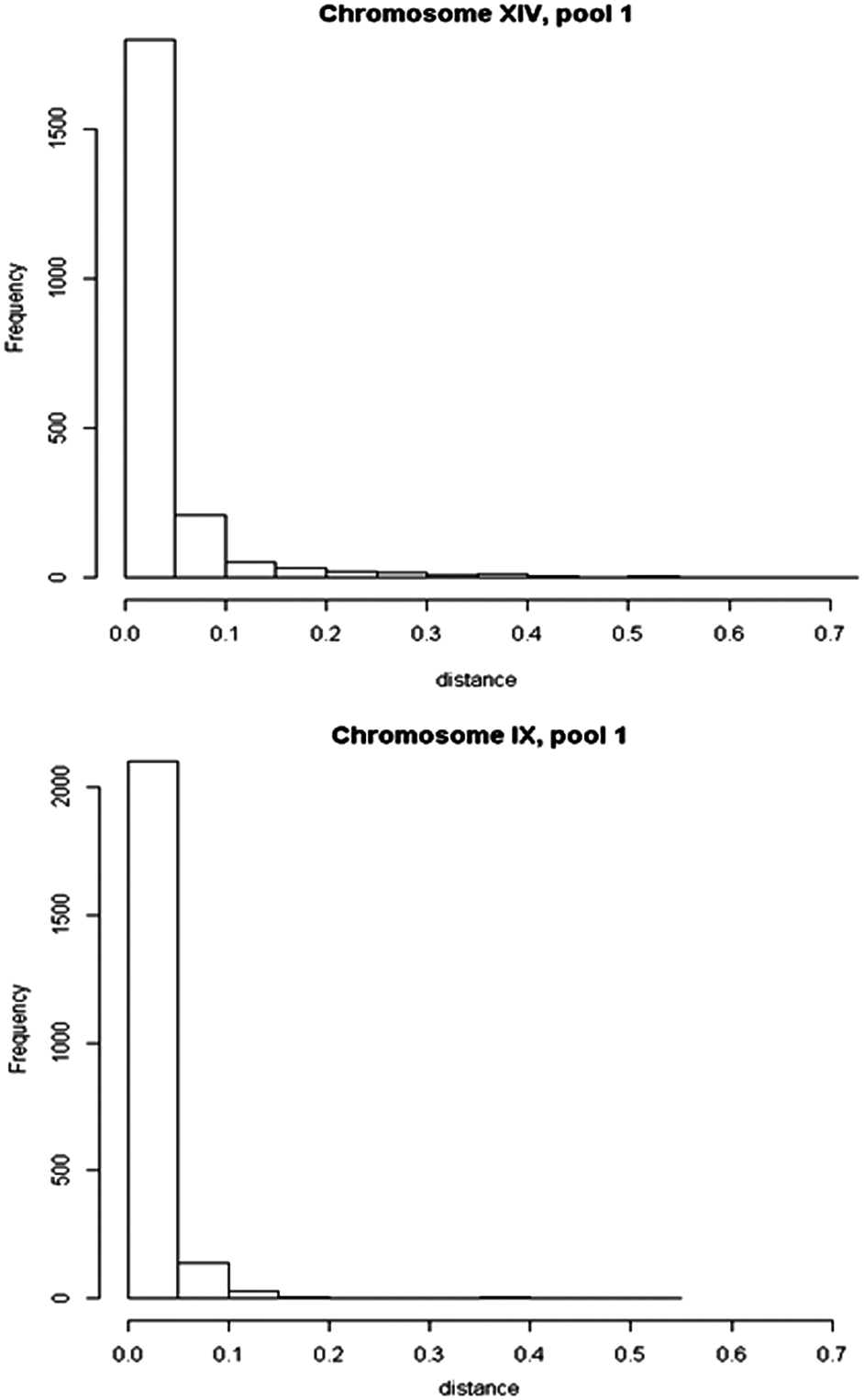
The histograms of distance (10 kbp) between neighboring SNPs in chromosome XIV, pool 1 (top panel), and chromosome IX, pool 1 (bottom panel). SNPs, single-nucleotide polymorphisms.

4.1. Chromosome XIV, pool 1

Table 1 shows the estimated concordance probabilities, initial probabilities, Akaike's information criterion (AIC), and Bayesian information criterion (BIC) for the H-HMM and NH-HMM.

Table 1.

Chromosome XIV, Pool 1: Comparison of Two Forms of the Hidden Markov Model with Three States and Their Corresponding Parameter Estimates (95% Confidence Intervals in Brackets)

Model	μ₁	μ₂	μ₃	δ₁	δ₂	δ₃	−log L_N	AIC	BIC
H-HMM	0.2269 [0.220, 0.230]	0.1284 [0.127, 0.129]	0.0559 [0.054, 0.056]	0^a	1^a	0^a	71,662.85	143,347.7	143,409.7
NH-HMM	0.2268 [0.220, 0.230]	0.1283 [0.127, 0.129]	0.0558 [0.054, 0.056]	0^a	1^a	0^a	71,638.09	143,298.2	143,360.1

Confidence interval could not be calculated as these parameters are at the boundary of the parameter space.

AIC, Akaike's information criterion; BIC, Bayesian information criterion; H-HMM, homogeneous hidden Markov model; NH-HMM, nonhomogeneous hidden Markov model.

The comparison of the first and the second row of Table 1 reveals that on the basis of the information criteria, the NH-HMM is worth considering. Note that the estimates of the concordance probabilities μ_j are almost similar for both models. In particular, based on the NH-HMM, the total probabilities of discordance between the reference parent and the offspring with high ethanol tolerance can be estimated to be equal to 1–4 × 0.2268 = 0.0928, 1–4 × 0.128 = 0.488, and 1–4 × 0.0559 = 0.776 for the first, second, and third state, respectively. Thus, following the reasoning outlined in Section 3.3, the first state can be seen as corresponding to SNPs linked with a gene locus of the parent without the trait, the second state can be considered as corresponding to the SNPs not linked with any genes, whereas the third state can be seen as SNPs that are potentially linked to one or more genes responsible to high ethanol tolerance.

Table 2 shows the estimated coefficients of the logit link function (4) describing the dependence of the transition probabilities on the distance between the adjacent SNPs (in 10 kbp). The estimated transition probabilities of the Markov chain, as a function of the distance between SNPs, are shown in Figure 3. The estimated coefficients indicate that, conditional on being in state 1, increasing the distance to the neighboring SNP increases the probability of transition to the second state. Similarly, for state 2, the larger the distance between the adjacent SNPs, the higher the chance of transition to state 3 as compared to state 1. For state 3, results similar to those for state 1 are obtained: increasing the distance between SNPs increases the probability of transition to the second state. In other words, for all three states, increasing the distance between the neighboring SNPs increases the chance of transition to another state. As a consequence, the transition probabilities of staying in the same state decrease as the distance between the neighboring SNPs increases. For state 1 (Fig. 3) this decline is especially large as compared to SNPs in states 2 and 3. The small number of SNPs, less densely spread out along the chromosome with SNPs frequency below 20% (Fig. 4), is most likely responsible for this effect. On the other hand, the probability of co-segregation decreases as the distance between the adjacent SNPs increases. The presence of QTLs for high ethanol tolerance in state 3 could be a possible reason for the high chance of transition from state 2 to 3 and from state 3 to 2 over large distances.

FIG. 3.

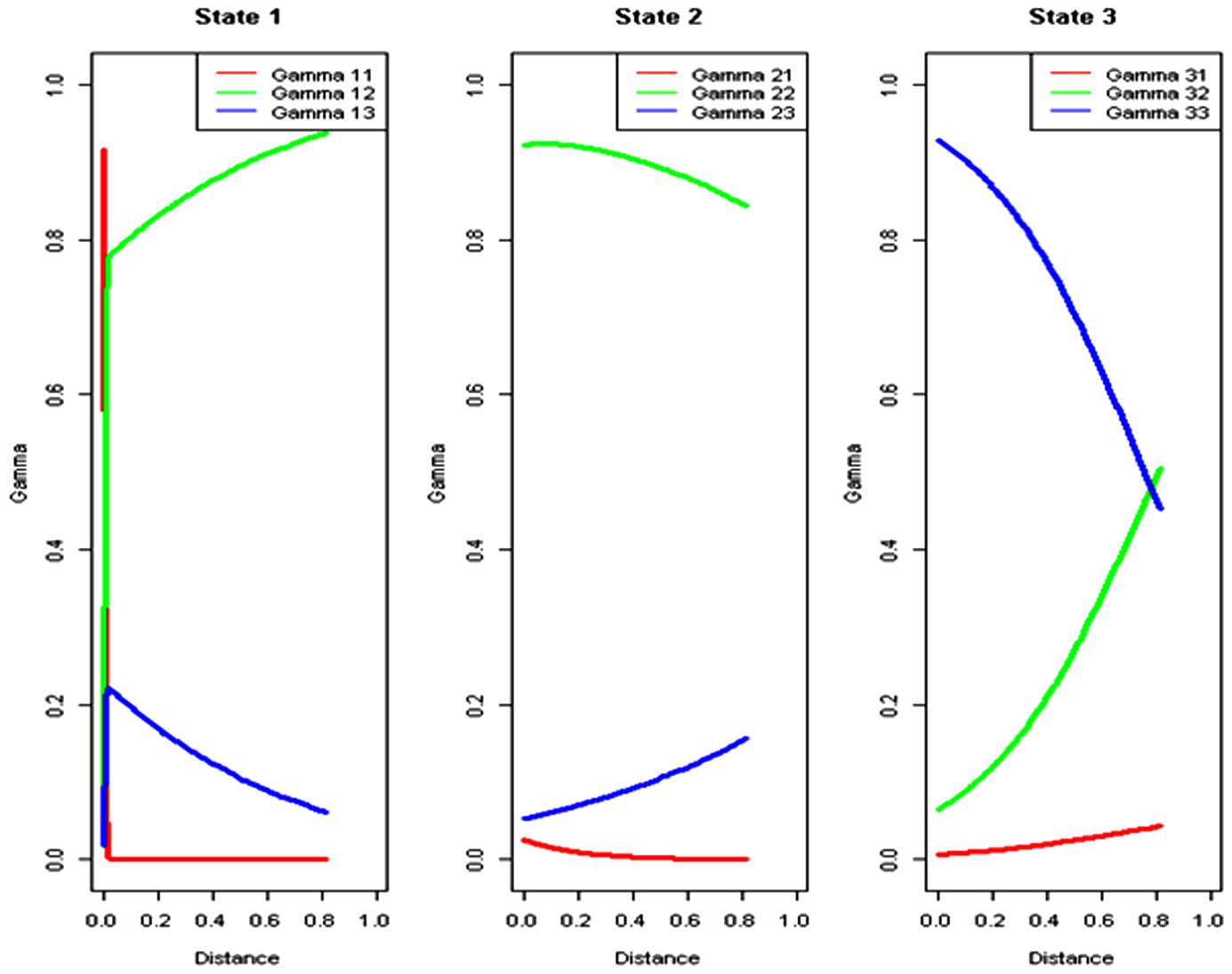
Probabilities of transition from one state to another, as estimated by the three-state nonhomogeneous HMM for chromosome XIV, pool 1.

FIG. 4.

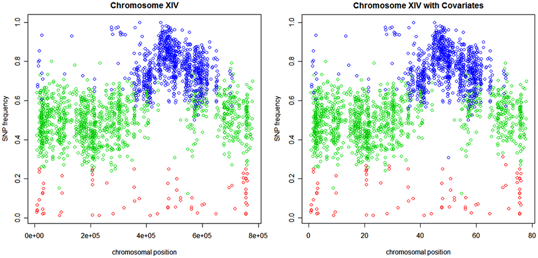
Chromosome XIV, pool 1, predicted SNP-specific states for the model with homogeneous HMM (left panel) and with nonhomogeneous HMM (right panel). Red stands for state 1, green for state 2, and blue for state 3.

Table 2.

Parameter Estimates (95% Confidence Intervals in Brackets) for the Nonhomogeneous Hidden Markov Model with Three States for Pool 1 of Chromosome XIV

Parameters	j = 1	j = 2	j = 3
α_j ₁	0	−3.591 [−4.055, −3.126]	−4.93 [−5.776, −4.084]
α_j ₂	−2.705 [−4.088, −1.323]	0	−2.668 [−2.950, −2.385]
α_j ₃	−3.926 [−5.483, −2.369]	−2.866 [−3.149, −2.583]	0
β_j ₁	0	−4.834 [−14.476, 4.806]	3.167 [−2.939, 9.273]
β_j ₂	438.909 [177.203,700.616]	0	3.402 [1.184, 5.619]
β_j ₃	437.078 [175.235,698.921]	1.444 [−1.074, 3.964]	0

The left-hand-side panel of Figure 4 presents the states predicted for each SNP based on the most likely state sequence (Viterbi algorithm) obtained from the fitted NH-HMM (Table 2), while the right-hand-side panel presents the states predicted for each SNP obtained from the NH-HMM. Both plots clearly illustrate that state 3 (blue) is associated with a high frequency of mismatched nucleotides, state 2 (green) with an intermediate frequency, and state 1 (red) with a low frequency. Except in few cases (10 SNPs), NH-HMM and H-HMM assign the SNPs to the same states.

4.2. Chromosome XIV, pool 2

Table 3 shows the results for the H-HMM and NH-HMM for pool 2 of chromosome XIV. The corresponding total discordance probabilities are equal to 0.321, 0.609, and 0.876 for state 1, state 2, and state 3, respectively. Table 4 shows the estimated coefficients of the logit link function describing the dependence of the transition probabilities on the distance between the adjacent SNPs (in 10 kbp) for the NH-HMM. It can be observed that (see Fig. 5), similarly to pool 1, the probabilities of staying in the same state decrease as the distance between the neighboring SNPs increases. However, for state 1 of pool 2, this decline is not as large as for pool 1 (see Fig. 3). The larger number of SNPs around 200,000 bp, due to the presence of a minor QTL, could be a possible reason for this behavior (Fig. 6). If the distance between SNPs increases, the possibility of moving from state 2 to state 3 and for state 3 to 2 also increases. Except for 10 SNPs, NH-HMM and H-HMM assign the SNPs to the same states (see Fig. 6).

FIG. 5.

Probabilities of transition from one state to another, as estimated by the three-state nonhomogeneous HMM for chromosome XIV, pool 2.

FIG. 6.

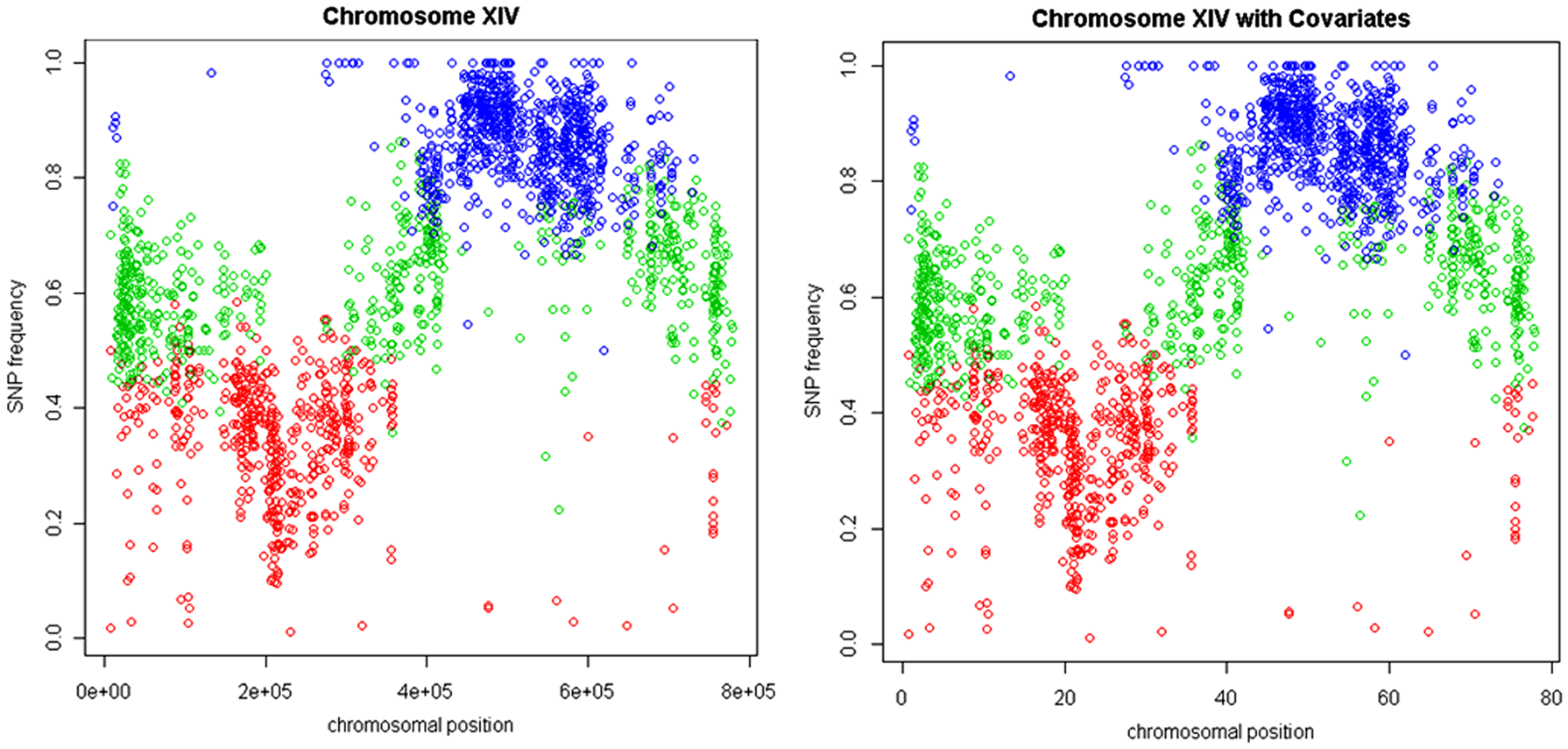
Chromosome XIV, pool 2, predicted SNP-specific states for the model with homogeneous HMM (left panel) and with nonhomogeneous HMM (right panel). Red stands for state 1, green for state 2, and blue for state 3.

Table 3.

Chromosome XIV, Pool 2: Comparison of Two Forms of the Hidden Markov Model with Three States and Their Corresponding Parameter Estimates (95% Confidence Intervals in Brackets)

Model	μ₁	μ₂	μ₃	δ₁	δ₂	δ₃	−log L_N	AIC	BIC
H-HMM	0.1696 [0.168,0.171]	0.0979 [0.096,0.099]	0.0309 [0.029,0.032]	1^a	0^a	0^a	74,749.81	149,521.6	149,583.6
NH-HMM	0.1695 [0.168,0.171]	0.0979 [0.168,0.171]	0.0308 [0.168,0.171]	1^a	0^a	0^a	74,739.59	149,501.2	149,563.1

Confidence interval could not be calculated as these parameters are at the boundary of the parameter space.

Table 4.

Parameter Estimates (95% Confidence Intervals in Brackets) for the Nonhomogeneous Hidden Markov Model with Three States of Pool 2 of Chromosome XIV

Parameters	j = 1	j = 2	j = 3
α_j ₁	0	−2.0530 [−2.324, −1.781]	−5.2343 [−6.163, −4.305]
α_j ₂	−2.0421 [−2.323, −1.76]	0	−2.8260 [−3.130, −2.516]
α_j ₃	−4.1373 [−4.868, −3.406]	−2.3521 [−2.660, −2.043]	0
β_j ₁	0	0.9012 [−1.529, 3.331]	8.0646 [4.057, 12.071]
β_j ₂	3.4682 [0.663, 6.273]	0	5.646201 [3.095, 8.197]
β_j ₃	4.5416 [−0.671, 9.755]	1.1887 [−1.414, 3.792]	0

5. Conclusions

In this article, we have presented an NH-HMM model for QTL mapping. The approach adopted by the NH-HMM has a number of advantages over a homogeneous HMM. Most importantly, by taking into account the distance between adjacent SNPs, an NH-HMM better models chromosomes where some regions are densely covered and others are covered at lower density. In addition, an NH-HMM can be extended to include other covariates except the distance between the adjacent SNPs. However, further investigation should be devoted to the choice of the relevant covariates for the NH-HMM. One of the main concerns in an NH-HMM model is choosing a suitable link function together with an appropriate distance scale. For instance, in our case, we choose the standard (multinomial) logit link function between covariates and the transition probabilities. Other link functions, such as probit, are also possible. In our analysis, the distance scale of 10 kbp between the adjacent SNPs was used.

Another important issue for using the NH-HMM is the number of parameters in the model that have to be estimated. Applying the NH-HMM can increase the number of estimated parameters related to the transition probabilities. For larger number of states, the number of these parameters increases the computation time of the forward–backward algorithm.

To decide which stochastic model fits the data best, AIC and BIC can be computed. In our case, there was a slight difference between the values of these information criteria for the basic HMM and the NH-HMM. Moreover, there was little difference in the estimated values of the parameters of interest, that is, the concordance probabilities. Thus, in our application, the results did not depend on the assumption of (non)homogeneity of the transition matrix.

Footnotes

Acknowledgments

The authors are grateful to Steve Swinnen, Thiago Pais, Maria R. Foulquie-Moreno, and Johan M. Thevelein of the Laboratory of Molecular Cell Biology, Institute of Botany and Microbiology, KU Leuven, and Department of Molecular Microbiology, VIB (Flemish Institute for Biotechnology), for providing the data. The authors gratefully acknowledge the support from the IAP Research Network P7/06 of the Belgian State (Belgian Science Policy).

Author Disclosure Statement

No competing financial interests exist.

References

Baum

L.E.

, Petrie

, Soules

, et al. 1970. A maximization technique occurring in the statistical analysis of probabilistic functions in Markov chains. Ann. Math. Stat. 41, 164–171.

Bellone

, Hughes

J.P.

, and Guttorp

2000. A hidden Markov model for downscaling synoptic atmospheric patterns to precipitation amounts. Clim. Res. 15, 1–12.

Betrò

, Bodini

, and Cossu

Q.A.

2008. Using hidden Markov model to analyze extreme rainfall events in Central-East Sardinia. Envirionmetrics, 19, 702–713.

Charles

S.P.

, Bates

B.C.

, and Hughes

J.P.

1999. A spatiotemporal model for downscaling precipitation occurrence and amounts. J. Geophys. Res. 104, 31657–31669.

Charles

S.P.

, Bates

B.C.

, Smith

I.N.

, et al. 2004. Statistical downscaling of daily precipitation from observed and modelled atmospheric fields. Hydrol. Processes, 18, 1373–1394.

Claesen

, and Burzykowski

, 2014. A hidden Markov-model for gene mapping based on whole genome sequencing data. Stat. Appl. Genet. Mol. Biol. [Epub ahead of print]; doi: 10.1515/sagmb-2014-0007.

Dempster

A.P.

, Laird

N.M.

, and Rubin

D.B.

1977. Maximum likelihood from incomplete data via the EM algorithm. J.R. Stat. Soc. B., 39, 1–38.

Dohm

J.C.

, Lottaz,C., Borodina

, et al. 2008. Substantial biases in ultra-short read data sets from high-throughput DNA sequences. Nucleic Acids Res., 36, e105.

Hughes

J.P.

1993. Disturbance effects on coral reef dynamics. Coral Reefs, 12, 115–234.

10.

Hughes

J.P.

, and Guttorp

1994. A class of stochastic models for relating synoptic atmospheric patterns to regional hydrologic phenomena. Water Resour. Res., 30, 1535–1546.

11.

Hughes

J.P.

, Guttorp

, and Charles

S.P.

1999. A non-homogeneous hidden Markov model for precipitation occurrence. Appl. Stat., 48, 15–30.

12.

Louis

T.A.

1982. Finding the observed information matrix when using the EM algorithm. J.R. Stat. Soc. B., 44, 226–233.

13.

MacDonald

I.L.

, and Zucchini

1997. Hidden Markov and Other Models for Discrete Valued Time Series. Chapman & Hall, London.

14.

Robertson

A.W.

, Kirshner

, and Smyth

2004. Downscaling of daily rainfall occurrence over Northeast Brazil using a hidden Markov model. J. Clim., 17, 4407–4424.

15.

Schneeberger

, Ossowski

, Lanz

, et al. 2009. SHOREmap: simultaneous mapping and mutation identification by deep sequencing. Nat. Methods, 6, 550–551.

16.

Shendure

, and Ji

2005. Next-generation DNA sequencing. Nat. Biotechnol., 26, 1135–1145.

17.

Swinnen

, Schaerlaekens

, Pais

, et al. 2012a. Identification of novel causative genes determining the complex trait of high ethanol tolerance in yeast using pooled segregant whole-genome sequence analysis. Genome Res. 22, 975–984.

18.

Swinnen

, Thevelein

J.M.

, and Nevoigt

2012b. Genetic mapping of quantitative phenotypic traits in Saccharomyces cerevisiae. FEMS Yeast Res., 12, 215–227.

19.

Viterbi

A.J.

1967. Error bounds for convolutional codes and an asymptotically optimum decoding algorithm. IEEE Trans. Inf. Theory, 13, 260–269.

20.

Zucchini

, and Guttorp

1991. A hidden Markov model for space-time precipitation. Water Resour. Res. 27, 1917–1923.

21.

Zucchini

, and MacDonald

I.L.

2009. Hidden Markov Models for Time Series. An Introduction Using R. CRC Press, Boca Raton, FL.

Supplementary Material

Please find the following supplemental material available below.

For Open Access articles published under a Creative Commons License, all supplemental material carries the same license as the article it is associated with.

For non-Open Access articles published, all supplemental material carries a non-exclusive license, and permission requests for re-use of supplemental material or any part of supplemental material shall be sent directly to the copyright owner as specified in the copyright notice associated with the article.

0.00 MB

0.03 MB