We introduce the concept of RNA multistructures, which is a formal grammar–based framework specifically designed to model a set of alternate RNA secondary structures. Such alternate structures can either be a set of suboptimal foldings, or distinct stable folding states, or variants within an RNA family. We provide several such examples and propose an efficient algorithm to search for RNA multistructures within a genomic sequence.
1. Introduction
Structural RNAs play important roles in a wide range of cellular processes, including protein synthesis, gene expression regulation, and more. In many RNA families the spatial architecture of the molecule is an important component of its function (Brosnan and Voinnet, 2009; Mattick and Makunin, 2006). This spatial architecture is mainly built upon the set of base pairings, which is captured in the secondary structure. Over the years, a great number of computational methods have been proposed to model consensus secondary structures. In many cases however, the signature for an RNA family cannot be compiled into a single consensus structure and is mainly given by a set of alternate secondary structures. For example, certain classes of RNAs adopt at least two distinct stable folding states to carry out their function. This is the case of riboswitches, which undergo structural changes upon binding with other molecules (Edwards and Batey, 2010), and recently some other RNA regulators were proven to show evolutionary evidence for alternative structure (Ritz et al., 2013). The necessity to take into account multiple structures also arises when modeling an RNA family with some structural variation across species, or when it comes to work with a set of predicted suboptimal foldings.
The objective of this article is to propose a computational method to deal efficiently with such sets of alternate secondary structures. We introduce the formal concept of RNA multistructures, which represent a set of alternate RNA secondary structures in a compact and nonredundant way. The definition uses formal grammars. Grammars have been applied extensively to the problem of RNA folding, aligning, and homology searching (Nawrocki et al., 2009; Hofacker and Stadler, 2014; Giegerich and Touzet, 2014). Compared to other tools from language theory, such as deterministic finite automata and HMMs, they are the method of choice because they are able to model long-range interactions. Here we exploit the power of this formalism to encode alternative foldings. The article is organized as follows. In Section 2, we briefly recall some basic definitions. Section 3 introduces the definition of RNA multistructures. Section 4 presents some examples to illustrate the utility of the concept. Lastly, in section 5, we describe an algorithm to search for an RNA multistructure in a genomic sequence.
2. RNA Secondary Structures
Throughout this article, we see RNA secondary structures as pure combinatorial objects composed of helices. Assume we have a linear sequence α provided with totally ordered positions. An interval is a pair of positions 〈x, y〉 of α such that x ≤ y. The interval 〈x, y〉 precedes the interval 〈x′, y′〉 if y < x′. A helix h is a pair of intervals 〈x, y〉 and 〈x′, y′〉 such that 〈x, y〉 precedes 〈x′, y′〉. So a helix is characterized by four positions on α, denoted h.5start, h.5end, h.3start, h.3end for x, y, x′ and y′ respectively. With this definition, a helix can contain unpaired positions, internal loops, or bulges, as illustrated in Figure 1. We say that the helix g is nested in the helix h if h.5end < g.5start and g.3end < h.3start. We say g is juxtaposed with h if g.3end < h.5start. A secondary structure is a set of helices that are all pairwise nested or juxtaposed. Note that in general any relation between two helices is authorized: They can overlap, form a pseudoknot, or be included in each other (See Fig. 2).
Several examples of the so-called helices: (a) all positions in the helix are paired, (b) helix with an internal symmetric loop, and (c) helix with a bulge. All these three types of helix are abstracted as a pair of intervals.
(a) Two nested helices, (b) two juxtaposed helices, (c) two overlapping helices, (d) two crossing helices that form a pseudoknot, and (e) a helix included in another helix.
3. RNA Multistructures
Before proceeding to the formal definition, we illustrate our motivation with a simple example taken from the human mitochondrial tRNA sequence. This sequence is 69 nt long and has eight thermodynamically stable helices, which are represented in Figure 3a. We denote this set of helices \documentclass{aastex}\usepackage{amsbsy}\usepackage{amsfonts}\usepackage{amssymb}\usepackage{bm}\usepackage{mathrsfs}\usepackage{pifont}\usepackage{stmaryrd}\usepackage{textcomp}\usepackage{portland, xspace}\usepackage{amsmath, amsxtra}\pagestyle{empty}\DeclareMathSizes{10}{9}{7}{6}\begin{document}
$$t{ \cal RN A}$$
\end{document}. The elements of \documentclass{aastex}\usepackage{amsbsy}\usepackage{amsfonts}\usepackage{amssymb}\usepackage{bm}\usepackage{mathrsfs}\usepackage{pifont}\usepackage{stmaryrd}\usepackage{textcomp}\usepackage{portland, xspace}\usepackage{amsmath, amsxtra}\pagestyle{empty}\DeclareMathSizes{10}{9}{7}{6}\begin{document}
$$t{ \cal RN A}$$
\end{document} can combine to form a variety of secondary structures. The question that we want to address is: How do you encode this set of secondary structures, or a given subset of these secondary structures, into a single compact data structure? Furthermore, we want to take advantage of the redundancy between the structures, since the structures may share some structural modules, and we want the data structure to be efficiently used for further queries.
Human mitochondrial tRNA sequence [source: FJ004809.1/12137–12205–RFAM, RF0005 (Burge et al., 2013)]. (a) Helices are numbered from 1 to 8 from 5′ to 3′, and are written in Vienna bracket–dot format. They are also represented as a set of pairs of intervals. (b) Helix graph. (c) Directed helix graph: h —▸g means that g is juxtaposed with h, and h --⊳ g means that g is nested in h.
In first approach, the set of helices \documentclass{aastex}\usepackage{amsbsy}\usepackage{amsfonts}\usepackage{amssymb}\usepackage{bm}\usepackage{mathrsfs}\usepackage{pifont}\usepackage{stmaryrd}\usepackage{textcomp}\usepackage{portland, xspace}\usepackage{amsmath, amsxtra}\pagestyle{empty}\DeclareMathSizes{10}{9}{7}{6}\begin{document}
$$t{ \cal RN A}$$
\end{document} can be represented by a graph, called the helix graph, whose vertices are helices, and there is an edge between every two vertices if helices are either juxtaposed, or nested. This graph is represented in Figure 3b. In this graph, the set of all secondary structures coincides with the set of cliques. However, this representation does not convey the necessary information to understand the topology of the set of helices. A better approach is to classify edges in two categories. This is what is done in the directed graph of Figure 3c. Plain arcs are for juxtaposed helices, and dotted arcs are for nested helices. Arcs are oriented in the same direction as the 3start positions on the underlying sequence α. In this graph, any secondary structure can be seen as a selection of plain paths, such that any two plain paths are linked by dotted paths. Each plain path characterizes a flat structure.
Definition 1.A set of helices w is a flat structure if, for any two distinct helices h and g in w, h and g are juxtaposed.
It is clear that any secondary structure can be partitioned into flat structures. We say that a flat structure w is nested into a helix h if all helices of w are nested into h. We define a multistructure as a combination of flat structures generated by a tree grammar.
Definition 2.A multistructure is a pair\documentclass{aastex}\usepackage{amsbsy}\usepackage{amsfonts}\usepackage{amssymb}\usepackage{bm}\usepackage{mathrsfs}\usepackage{pifont}\usepackage{stmaryrd}\usepackage{textcomp}\usepackage{portland, xspace}\usepackage{amsmath, amsxtra}\pagestyle{empty}\DeclareMathSizes{10}{9}{7}{6}\begin{document}
$${ \cal M} = ( { \cal H , G} )$$
\end{document}, where\documentclass{aastex}\usepackage{amsbsy}\usepackage{amsfonts}\usepackage{amssymb}\usepackage{bm}\usepackage{mathrsfs}\usepackage{pifont}\usepackage{stmaryrd}\usepackage{textcomp}\usepackage{portland, xspace}\usepackage{amsmath, amsxtra}\pagestyle{empty}\DeclareMathSizes{10}{9}{7}{6}\begin{document}
$${ \cal H}$$
\end{document}is a set of helices and\documentclass{aastex}\usepackage{amsbsy}\usepackage{amsfonts}\usepackage{amssymb}\usepackage{bm}\usepackage{mathrsfs}\usepackage{pifont}\usepackage{stmaryrd}\usepackage{textcomp}\usepackage{portland, xspace}\usepackage{amsmath, amsxtra}\pagestyle{empty}\DeclareMathSizes{10}{9}{7}{6}\begin{document}
$${ \cal G}$$
\end{document}is a tree grammar. The grammar alphabet contains a start symbol S, a binary terminal symbol\documentclass{aastex}\usepackage{amsbsy}\usepackage{amsfonts}\usepackage{amssymb}\usepackage{bm}\usepackage{mathrsfs}\usepackage{pifont}\usepackage{stmaryrd}\usepackage{textcomp}\usepackage{portland, xspace}\usepackage{amsmath, amsxtra}\pagestyle{empty}\DeclareMathSizes{10}{9}{7}{6}\begin{document}
$$\circ$$
\end{document}, and for each helix h of\documentclass{aastex}\usepackage{amsbsy}\usepackage{amsfonts}\usepackage{amssymb}\usepackage{bm}\usepackage{mathrsfs}\usepackage{pifont}\usepackage{stmaryrd}\usepackage{textcomp}\usepackage{portland, xspace}\usepackage{amsmath, amsxtra}\pagestyle{empty}\DeclareMathSizes{10}{9}{7}{6}\begin{document}
$${ \cal H}$$
\end{document}, a nonterminal symbol H and a terminal symbol h. All its productions are of the form\documentclass{aastex}\usepackage{amsbsy}\usepackage{amsfonts}\usepackage{amssymb}\usepackage{bm}\usepackage{mathrsfs}\usepackage{pifont}\usepackage{stmaryrd}\usepackage{textcomp}\usepackage{portland, xspace}\usepackage{amsmath, amsxtra}\pagestyle{empty}\DeclareMathSizes{10}{9}{7}{6}\begin{document}
\begin{align*} ( 1 ) \quad & S \rightarrow H_1 \circ \ldots \circ H_q \\ ( 2 ) \quad & H \rightarrow h ( H_1 \circ \ldots \circ H_q ) \\ ( 3 ) \quad & H \rightarrow h\end{align*}
\end{document}
where\documentclass{aastex}\usepackage{amsbsy}\usepackage{amsfonts}\usepackage{amssymb}\usepackage{bm}\usepackage{mathrsfs}\usepackage{pifont}\usepackage{stmaryrd}\usepackage{textcomp}\usepackage{portland, xspace}\usepackage{amsmath, amsxtra}\pagestyle{empty}\DeclareMathSizes{10}{9}{7}{6}\begin{document}
$$h_1 \circ \ldots \circ h_q$$
\end{document}is any flat structure on\documentclass{aastex}\usepackage{amsbsy}\usepackage{amsfonts}\usepackage{amssymb}\usepackage{bm}\usepackage{mathrsfs}\usepackage{pifont}\usepackage{stmaryrd}\usepackage{textcomp}\usepackage{portland, xspace}\usepackage{amsmath, amsxtra}\pagestyle{empty}\DeclareMathSizes{10}{9}{7}{6}\begin{document}
$${ \cal H}$$
\end{document}in (1), and a flat structure that is nested in h in (2).
In the definition of \documentclass{aastex}\usepackage{amsbsy}\usepackage{amsfonts}\usepackage{amssymb}\usepackage{bm}\usepackage{mathrsfs}\usepackage{pifont}\usepackage{stmaryrd}\usepackage{textcomp}\usepackage{portland, xspace}\usepackage{amsmath, amsxtra}\pagestyle{empty}\DeclareMathSizes{10}{9}{7}{6}\begin{document}
$${ \cal G}$$
\end{document}, \documentclass{aastex}\usepackage{amsbsy}\usepackage{amsfonts}\usepackage{amssymb}\usepackage{bm}\usepackage{mathrsfs}\usepackage{pifont}\usepackage{stmaryrd}\usepackage{textcomp}\usepackage{portland, xspace}\usepackage{amsmath, amsxtra}\pagestyle{empty}\DeclareMathSizes{10}{9}{7}{6}\begin{document}
$$H_1 \circ \ldots \circ H_q$$
\end{document} indicates which plain paths from the helix graph are authorized in the multistructure, and \documentclass{aastex}\usepackage{amsbsy}\usepackage{amsfonts}\usepackage{amssymb}\usepackage{bm}\usepackage{mathrsfs}\usepackage{pifont}\usepackage{stmaryrd}\usepackage{textcomp}\usepackage{portland, xspace}\usepackage{amsmath, amsxtra}\pagestyle{empty}\DeclareMathSizes{10}{9}{7}{6}\begin{document}
$$h ( \ldots )$$
\end{document} indicates which dotted paths are authorized in the multistructure. The \documentclass{aastex}\usepackage{amsbsy}\usepackage{amsfonts}\usepackage{amssymb}\usepackage{bm}\usepackage{mathrsfs}\usepackage{pifont}\usepackage{stmaryrd}\usepackage{textcomp}\usepackage{portland, xspace}\usepackage{amsmath, amsxtra}\pagestyle{empty}\DeclareMathSizes{10}{9}{7}{6}\begin{document}
$$\circ$$
\end{document} symbol allows to generate trees of arbitrary arity. An instance of the multistructure \documentclass{aastex}\usepackage{amsbsy}\usepackage{amsfonts}\usepackage{amssymb}\usepackage{bm}\usepackage{mathrsfs}\usepackage{pifont}\usepackage{stmaryrd}\usepackage{textcomp}\usepackage{portland, xspace}\usepackage{amsmath, amsxtra}\pagestyle{empty}\DeclareMathSizes{10}{9}{7}{6}\begin{document}
$${ \cal M}$$
\end{document} is any structure recognized by its grammar \documentclass{aastex}\usepackage{amsbsy}\usepackage{amsfonts}\usepackage{amssymb}\usepackage{bm}\usepackage{mathrsfs}\usepackage{pifont}\usepackage{stmaryrd}\usepackage{textcomp}\usepackage{portland, xspace}\usepackage{amsmath, amsxtra}\pagestyle{empty}\DeclareMathSizes{10}{9}{7}{6}\begin{document}
$${ \cal G}$$
\end{document}. It is straightforward to verify that each instance of a multistructure is a secondary structure.
By construction, the language of this grammar is exactly the set of all secondary structures on \documentclass{aastex}\usepackage{amsbsy}\usepackage{amsfonts}\usepackage{amssymb}\usepackage{bm}\usepackage{mathrsfs}\usepackage{pifont}\usepackage{stmaryrd}\usepackage{textcomp}\usepackage{portland, xspace}\usepackage{amsmath, amsxtra}\pagestyle{empty}\DeclareMathSizes{10}{9}{7}{6}\begin{document}
$$t{ \cal RN A}$$
\end{document}. The reader is invited to check that it contains 43 structures.
We take this example a step further and address the problem of building a multistructure for all locally optimal secondary structures on \documentclass{aastex}\usepackage{amsbsy}\usepackage{amsfonts}\usepackage{amssymb}\usepackage{bm}\usepackage{mathrsfs}\usepackage{pifont}\usepackage{stmaryrd}\usepackage{textcomp}\usepackage{portland, xspace}\usepackage{amsmath, amsxtra}\pagestyle{empty}\DeclareMathSizes{10}{9}{7}{6}\begin{document}
$$t{ \cal RN A}$$
\end{document}. A locally optimal secondary structure is a secondary structure to which it is not possible to add a supplementary helix (Clote, 2005; Saffarian et al., 2012). In other words, it is a maximal clique in our helix graph of Figure 3. Figure 4 represents all locally optimal secondary structures for \documentclass{aastex}\usepackage{amsbsy}\usepackage{amsfonts}\usepackage{amssymb}\usepackage{bm}\usepackage{mathrsfs}\usepackage{pifont}\usepackage{stmaryrd}\usepackage{textcomp}\usepackage{portland, xspace}\usepackage{amsmath, amsxtra}\pagestyle{empty}\DeclareMathSizes{10}{9}{7}{6}\begin{document}
$$t{ \cal RN A}$$
\end{document}. In Saffarian et al. (2012), we have proved that locally optimal secondary structures are exactly the secondary structures that are partitioned into some maximal flat structures, called maximal for juxtaposition, and corresponding to some maximal plain paths in the helix graph.
Locally optimal secondary structures for the set of helices \documentclass{aastex}\usepackage{amsbsy}\usepackage{amsfonts}\usepackage{amssymb}\usepackage{bm}\usepackage{mathrsfs}\usepackage{pifont}\usepackage{stmaryrd}\usepackage{textcomp}\usepackage{portland, xspace}\usepackage{amsmath, amsxtra}\pagestyle{empty}\DeclareMathSizes{10}{9}{7}{6}\begin{document}
$$t{ \cal RN A}$$
\end{document} introduced in Figure 3.
Definition 3.(adapted from Saffarian et al., 2012) Given a set of helices \documentclass{aastex}\usepackage{amsbsy}\usepackage{amsfonts}\usepackage{amssymb}\usepackage{bm}\usepackage{mathrsfs}\usepackage{pifont}\usepackage{stmaryrd}\usepackage{textcomp}\usepackage{portland, xspace}\usepackage{amsmath, amsxtra}\pagestyle{empty}\DeclareMathSizes{10}{9}{7}{6}\begin{document}
$${ \cal H}$$
\end{document}, a flat structure w is maximal for juxtaposition if it satisfies the following condition: for each helix f of\documentclass{aastex}\usepackage{amsbsy}\usepackage{amsfonts}\usepackage{amssymb}\usepackage{bm}\usepackage{mathrsfs}\usepackage{pifont}\usepackage{stmaryrd}\usepackage{textcomp}\usepackage{portland, xspace}\usepackage{amsmath, amsxtra}\pagestyle{empty}\DeclareMathSizes{10}{9}{7}{6}\begin{document}
$${ \cal H}$$
\end{document} not present in w, then f is contained into some helix of w, or if {f} ∪ w is a secondary structure, then f is nested in some helix of w. Here, this result allows to define \documentclass{aastex}\usepackage{amsbsy}\usepackage{amsfonts}\usepackage{amssymb}\usepackage{bm}\usepackage{mathrsfs}\usepackage{pifont}\usepackage{stmaryrd}\usepackage{textcomp}\usepackage{portland, xspace}\usepackage{amsmath, amsxtra}\pagestyle{empty}\DeclareMathSizes{10}{9}{7}{6}\begin{document}
$${ \cal G}_1$$
\end{document}.
\documentclass{aastex}\usepackage{amsbsy}\usepackage{amsfonts}\usepackage{amssymb}\usepackage{bm}\usepackage{mathrsfs}\usepackage{pifont}\usepackage{stmaryrd}\usepackage{textcomp}\usepackage{portland, xspace}\usepackage{amsmath, amsxtra}\pagestyle{empty}\DeclareMathSizes{10}{9}{7}{6}\begin{document}
\begin{align*}S & \rightarrow H_1 \\ H_1 & \rightarrow h_1 ( H_2 \circ H_5 \circ H_8 ) \ \mid \ h_1 ( H_2 \circ H_6 ) \ \mid \ h_1 ( H_3 ) \ \mid \ h_1 ( H_4 \circ H_8 ) \\ H_2 & \rightarrow h_2 \\ H_3 & \rightarrow h_3 ( H_4 \circ H_7 ) \ \mid \ h_3 ( H_5 ) \\ H_4 & \rightarrow h_4 \\ H_5 & \rightarrow h_5 \\ H_6 & \rightarrow h_6 ( H_7 ) \\ H_7 & \rightarrow h_7 \\ H_8 & \rightarrow h_8\end{align*}
\end{document}
By construction, \documentclass{aastex}\usepackage{amsbsy}\usepackage{amsfonts}\usepackage{amssymb}\usepackage{bm}\usepackage{mathrsfs}\usepackage{pifont}\usepackage{stmaryrd}\usepackage{textcomp}\usepackage{portland, xspace}\usepackage{amsmath, amsxtra}\pagestyle{empty}\DeclareMathSizes{10}{9}{7}{6}\begin{document}
$${ \cal G}_1$$
\end{document} generates exactly all locally optimal secondary structures of \documentclass{aastex}\usepackage{amsbsy}\usepackage{amsfonts}\usepackage{amssymb}\usepackage{bm}\usepackage{mathrsfs}\usepackage{pifont}\usepackage{stmaryrd}\usepackage{textcomp}\usepackage{portland, xspace}\usepackage{amsmath, amsxtra}\pagestyle{empty}\DeclareMathSizes{10}{9}{7}{6}\begin{document}
$$t{ \cal RN A}$$
\end{document}. The number of instances is 5: h1(h2\documentclass{aastex}\usepackage{amsbsy}\usepackage{amsfonts}\usepackage{amssymb}\usepackage{bm}\usepackage{mathrsfs}\usepackage{pifont}\usepackage{stmaryrd}\usepackage{textcomp}\usepackage{portland, xspace}\usepackage{amsmath, amsxtra}\pagestyle{empty}\DeclareMathSizes{10}{9}{7}{6}\begin{document}
$$\circ$$
\end{document}h5\documentclass{aastex}\usepackage{amsbsy}\usepackage{amsfonts}\usepackage{amssymb}\usepackage{bm}\usepackage{mathrsfs}\usepackage{pifont}\usepackage{stmaryrd}\usepackage{textcomp}\usepackage{portland, xspace}\usepackage{amsmath, amsxtra}\pagestyle{empty}\DeclareMathSizes{10}{9}{7}{6}\begin{document}
$$\circ$$
\end{document}h8), h1(h2\documentclass{aastex}\usepackage{amsbsy}\usepackage{amsfonts}\usepackage{amssymb}\usepackage{bm}\usepackage{mathrsfs}\usepackage{pifont}\usepackage{stmaryrd}\usepackage{textcomp}\usepackage{portland, xspace}\usepackage{amsmath, amsxtra}\pagestyle{empty}\DeclareMathSizes{10}{9}{7}{6}\begin{document}
$$\circ$$
\end{document}h6(h7)), h1(h3(h4\documentclass{aastex}\usepackage{amsbsy}\usepackage{amsfonts}\usepackage{amssymb}\usepackage{bm}\usepackage{mathrsfs}\usepackage{pifont}\usepackage{stmaryrd}\usepackage{textcomp}\usepackage{portland, xspace}\usepackage{amsmath, amsxtra}\pagestyle{empty}\DeclareMathSizes{10}{9}{7}{6}\begin{document}
$$\circ$$
\end{document}h7)), h1(h3(h5)), h1(h4\documentclass{aastex}\usepackage{amsbsy}\usepackage{amsfonts}\usepackage{amssymb}\usepackage{bm}\usepackage{mathrsfs}\usepackage{pifont}\usepackage{stmaryrd}\usepackage{textcomp}\usepackage{portland, xspace}\usepackage{amsmath, amsxtra}\pagestyle{empty}\DeclareMathSizes{10}{9}{7}{6}\begin{document}
$$\circ$$
\end{document}h8), which are the maximal cliques of Figure 4. As expected, none are included in each other.
Lastly, multistructures can be used to encode a predefined set of secondary structures. This time, we start from a set of candidate secondary structures with low free energy level. We ran the mfold software with 20% suboptimality (Zuker, 2003) on our tRNA sequence and obtained four suboptimal structures, shown in Figure 5. From this set of structures, we extracted the set of helices, which appears to be the helix set \documentclass{aastex}\usepackage{amsbsy}\usepackage{amsfonts}\usepackage{amssymb}\usepackage{bm}\usepackage{mathrsfs}\usepackage{pifont}\usepackage{stmaryrd}\usepackage{textcomp}\usepackage{portland, xspace}\usepackage{amsmath, amsxtra}\pagestyle{empty}\DeclareMathSizes{10}{9}{7}{6}\begin{document}
$$t{ \cal RN A}$$
\end{document}. To build the productions of the grammar \documentclass{aastex}\usepackage{amsbsy}\usepackage{amsfonts}\usepackage{amssymb}\usepackage{bm}\usepackage{mathrsfs}\usepackage{pifont}\usepackage{stmaryrd}\usepackage{textcomp}\usepackage{portland, xspace}\usepackage{amsmath, amsxtra}\pagestyle{empty}\DeclareMathSizes{10}{9}{7}{6}\begin{document}
$${ \cal G}_2$$
\end{document}, we consider for each helix h the flat structure composed of all helices connected to the multibranch loop closed by h.
\documentclass{aastex}\usepackage{amsbsy}\usepackage{amsfonts}\usepackage{amssymb}\usepackage{bm}\usepackage{mathrsfs}\usepackage{pifont}\usepackage{stmaryrd}\usepackage{textcomp}\usepackage{portland, xspace}\usepackage{amsmath, amsxtra}\pagestyle{empty}\DeclareMathSizes{10}{9}{7}{6}\begin{document}
\begin{align*}S & \rightarrow H_1 \\ H_1 & \rightarrow h_1 ( H_2 \circ H_5 \circ H_8 ) \ \mid \ h_1 ( H_2 \circ H_6 ) \ \mid \ h_1 ( H_3 ) \\ H_2 & \rightarrow h_2 \\ H_3 & \rightarrow h_3 ( H_4 \circ H_7 ) \ \mid \ h_3 ( H_5 ) \\ H_4 & \rightarrow h_4 \\ H_5 & \rightarrow h_5 \\ H_6 & \rightarrow h_6 ( H_7 ) \\ H_7 & \rightarrow h_7 \\ H_8 & \rightarrow h_8\end{align*}
\end{document}
M-fold output for the human mitochondrial tRNA sequence.
Compared to \documentclass{aastex}\usepackage{amsbsy}\usepackage{amsfonts}\usepackage{amssymb}\usepackage{bm}\usepackage{mathrsfs}\usepackage{pifont}\usepackage{stmaryrd}\usepackage{textcomp}\usepackage{portland, xspace}\usepackage{amsmath, amsxtra}\pagestyle{empty}\DeclareMathSizes{10}{9}{7}{6}\begin{document}
$${ \cal G}_1$$
\end{document}, the production H1 → h1(H4\documentclass{aastex}\usepackage{amsbsy}\usepackage{amsfonts}\usepackage{amssymb}\usepackage{bm}\usepackage{mathrsfs}\usepackage{pifont}\usepackage{stmaryrd}\usepackage{textcomp}\usepackage{portland, xspace}\usepackage{amsmath, amsxtra}\pagestyle{empty}\DeclareMathSizes{10}{9}{7}{6}\begin{document}
$$\circ$$
\end{document}H8) is missing since none of the four suboptimal structures contains this combination of helices. This new multistructure has four distinct instances that correspond exactly to the four suboptimal secondary structures of Figure 5: {1, 2, 6, 7}, {1, 3, 5}, {1, 2, 5, 8}, and {1, 3, 4, 7}. This construction is guaranteed to give all input structures. We will see in the subsection 4.3 on bacterial RNase P RNA that it can happen that some new instances are created by the grammar.
The two multistructures \documentclass{aastex}\usepackage{amsbsy}\usepackage{amsfonts}\usepackage{amssymb}\usepackage{bm}\usepackage{mathrsfs}\usepackage{pifont}\usepackage{stmaryrd}\usepackage{textcomp}\usepackage{portland, xspace}\usepackage{amsmath, amsxtra}\pagestyle{empty}\DeclareMathSizes{10}{9}{7}{6}\begin{document}
$${ \cal G}_1$$
\end{document} and \documentclass{aastex}\usepackage{amsbsy}\usepackage{amsfonts}\usepackage{amssymb}\usepackage{bm}\usepackage{mathrsfs}\usepackage{pifont}\usepackage{stmaryrd}\usepackage{textcomp}\usepackage{portland, xspace}\usepackage{amsmath, amsxtra}\pagestyle{empty}\DeclareMathSizes{10}{9}{7}{6}\begin{document}
$${ \cal G}_2$$
\end{document} can be computed from the sequence without knowing the actual secondary structure. They result from in silico prediction. Nevertheless, they can serve to improve homology searching, even if the real structure is not known: Build the associated multistructure, then use this multistructure to scan a genomic sequence in conjunction with sequence similarity.
4.2. Multistructure for the guanine riboswitch
Riboswitches are regulatory elements that are found in the untranslated regions of messenger RNA. They adopt alternate secondary structures depending on the binding of specific metabolites. This binding affects the translation of the gene, and thus participates to the regulation of its activity. Riboswitches are usually composed of two domains: The aptamer domain, which acts as a receptor that specifically binds the ligand, and the expression platform, which acts directly on gene expression. Figure 6 shows such an example—the guanine riboswitch in the xpt gene, which is involved in purine metabolism in Bacillus subtilis. The multistructure associated with the two conformational states is as follows.
\documentclass{aastex}\usepackage{amsbsy}\usepackage{amsfonts}\usepackage{amssymb}\usepackage{bm}\usepackage{mathrsfs}\usepackage{pifont}\usepackage{stmaryrd}\usepackage{textcomp}\usepackage{portland, xspace}\usepackage{amsmath, amsxtra}\pagestyle{empty}\DeclareMathSizes{10}{9}{7}{6}\begin{document}
\begin{align*}S & \rightarrow H_4 \ \mid \ H_1 \circ H_5 \circ H_6 \\ H_1 & \rightarrow h_1 ( H_2 \circ H_3 ) \\ H_2 & \rightarrow h_2 \\ H_3 & \rightarrow h_3 \\ H_4 & \rightarrow h_4 ( H_2 \circ H_3 \circ H_7 ) \\ H_5 & \rightarrow h_5 \\ H_6 & \rightarrow h_6 \\ H_7 & \rightarrow h_7 ( H_8 \circ H_9 ) \\ H_8 & \rightarrow h_8 \\ H_9 & \rightarrow h_9\end{align*}
\end{document}
Alternate configurations of the guanine riboswitch (source: Biological Physics at CMU, Mike Widom's lab). (a) In presence of the ligand, the aptamer forms (in green), and the terminator also forms (in red). As a result, the gene is switched off. (b) If the aptamer does not form, then the terminator is not formed, and the gene is switched on.
The variables h1, h2, and h3 constitute the aptamer domain and are refered as P1, P2, and P3 respectively, in the terminology of purine riboswitches: h1 is the aptamer (in green on the figure), and h2 and h3 bind the metabolite; h6 (in red in the figure) is the main element of the expression platform. It is a translation-terminating stem-loop, which forms in the presence of the ligand, when h1 is also formed. This grammar generates exactly two secondary structures, h1(h2\documentclass{aastex}\usepackage{amsbsy}\usepackage{amsfonts}\usepackage{amssymb}\usepackage{bm}\usepackage{mathrsfs}\usepackage{pifont}\usepackage{stmaryrd}\usepackage{textcomp}\usepackage{portland, xspace}\usepackage{amsmath, amsxtra}\pagestyle{empty}\DeclareMathSizes{10}{9}{7}{6}\begin{document}
$$\circ$$
\end{document}h3) \documentclass{aastex}\usepackage{amsbsy}\usepackage{amsfonts}\usepackage{amssymb}\usepackage{bm}\usepackage{mathrsfs}\usepackage{pifont}\usepackage{stmaryrd}\usepackage{textcomp}\usepackage{portland, xspace}\usepackage{amsmath, amsxtra}\pagestyle{empty}\DeclareMathSizes{10}{9}{7}{6}\begin{document}
$$\circ$$
\end{document}h5\documentclass{aastex}\usepackage{amsbsy}\usepackage{amsfonts}\usepackage{amssymb}\usepackage{bm}\usepackage{mathrsfs}\usepackage{pifont}\usepackage{stmaryrd}\usepackage{textcomp}\usepackage{portland, xspace}\usepackage{amsmath, amsxtra}\pagestyle{empty}\DeclareMathSizes{10}{9}{7}{6}\begin{document}
$$\circ$$
\end{document}h6, which is the off state, and h4(h2\documentclass{aastex}\usepackage{amsbsy}\usepackage{amsfonts}\usepackage{amssymb}\usepackage{bm}\usepackage{mathrsfs}\usepackage{pifont}\usepackage{stmaryrd}\usepackage{textcomp}\usepackage{portland, xspace}\usepackage{amsmath, amsxtra}\pagestyle{empty}\DeclareMathSizes{10}{9}{7}{6}\begin{document}
$$\circ$$
\end{document}h3\documentclass{aastex}\usepackage{amsbsy}\usepackage{amsfonts}\usepackage{amssymb}\usepackage{bm}\usepackage{mathrsfs}\usepackage{pifont}\usepackage{stmaryrd}\usepackage{textcomp}\usepackage{portland, xspace}\usepackage{amsmath, amsxtra}\pagestyle{empty}\DeclareMathSizes{10}{9}{7}{6}\begin{document}
$$\circ$$
\end{document}h7(h8\documentclass{aastex}\usepackage{amsbsy}\usepackage{amsfonts}\usepackage{amssymb}\usepackage{bm}\usepackage{mathrsfs}\usepackage{pifont}\usepackage{stmaryrd}\usepackage{textcomp}\usepackage{portland, xspace}\usepackage{amsmath, amsxtra}\pagestyle{empty}\DeclareMathSizes{10}{9}{7}{6}\begin{document}
$$\circ$$
\end{document}h9)), which is the on state. This clearly shows that these two states are mutually exclusive, and no other conformation is likely to form.
4.3. Multistructures for bacterial RNase P RNAs
In this example, we explain how to model an RNA family with a multistructure. Bacterial RNase P RNAs fall into two major classes that share a common catalytic core, but also show some distinct structural modules: type A (represented by Escherichia coli in Fig. 7) is the common and ancestral form found in most bacteria, and type B (represented by Bacillus subtilis in Fig. 7) is found in the low-GC content gram-positive bacteria (Haas and Brown, 1998). We explain how to gather the two structures in the same multistructure. Following the nomenclature of the RNase P database, helices are labeled P1 − P18 from 5′ to 3′ in the E. coli structure. Helices P4 and P6 form pseudoknots and do not belong to the secondary structure. B. subtilis features some additional helices, denoted P5.1, P10.1, P15.1, and P19, and lacks helices P13, P14, P16, and P17. The corresponding grammar is obtained by taking all flat structures of each of the two consensus secondary structures for type A and type B.
\documentclass{aastex}\usepackage{amsbsy}\usepackage{amsfonts}\usepackage{amssymb}\usepackage{bm}\usepackage{mathrsfs}\usepackage{pifont}\usepackage{stmaryrd}\usepackage{textcomp}\usepackage{portland, xspace}\usepackage{amsmath, amsxtra}\pagestyle{empty}\DeclareMathSizes{10}{9}{7}{6}\begin{document}
\begin{align*}S & \rightarrow P_1 \\ P_1 & \rightarrow p_1 ( P_2 ) \ \mid \ p_1 ( P_2 \circ P_{19} ) \\ P_2 & \rightarrow p_2 ( P_3 ) \ \mid \ p_2 ( P_3 \circ P_5 \circ P_{15} \circ P_{18} ) \ \mid \ p_2 ( P_3 \circ P_5 \circ P_{15} \circ P_{15.1} \circ P_{18} ) \\ P_3 & \rightarrow p_3 \\ P_5 & \rightarrow p_5 ( P_{5.1} \circ P_7 ) \ \mid \ p_5 ( P_7 ) \\ P_{5.1} & \rightarrow p_{5.1} \\ P_7 & \rightarrow p_7 ( P_8 \circ P_9 \circ P_{10} ) \\ P_8 & \rightarrow p_8 \\ P_9 & \rightarrow p_9 \\ P_{10} & \rightarrow p_{10} ( P_{10.1} \circ P_{11} ) \ \mid \ p_{11} \\ P_{10.1} & \rightarrow p_{10.1} \\ P_{11} & \rightarrow p_{11} ( P_{12} ) \ \mid \ p_{11} ( P_{12} \circ P_{13} \circ P_{14} ) \\ P_{12} & \rightarrow p_{12} \\ P_{13} & \rightarrow p_{13} \\ P_{14} & \rightarrow p_{14} \\ P_{15} & \rightarrow p_{15} ( P_{16} ) \ \mid \ p_{15} \\ P_{15.1} & \rightarrow p_{15.1} \\ P_{16} & \rightarrow p_{16} ( P_{17} ) \\ P_{17} & \rightarrow p_{17} \\ P_{18} & \rightarrow p_{18} \\ P_{19} & \rightarrow p_{19}\end{align*}
\end{document}
Secondary structures for bacterial RNase P RNA (source: Brown, 1999).
Green nonsulfur bacteria RNase P RNAs are known to show some notable variation against the forms A and B. The majority of them (represented here by H. auriantacus in Fig. 7) are of the type A class, except for the structural module P18/P15.1 that is instead quite similar to that of the type B and for the helix P19. One exception is represented by the sequence of T. roseum, which has independently converged with the class B RNAs (presence of helices P10.1 and P15.1, and absence of helices P13, P14, and P19). However, T. roseum RNA retains P16/P17 and does not contain P5.1 (Haas and Brown 1998) (see Fig. 7). Interestingly, these two variants appear as instances of the multistructure designed to encode solely types A and B. It means that in this example, these two new structures created by the multistructure are functional and have been selected by the evolution.
5. Searching multistructures in genomic sequences
We now turn to the following problem: Given a multistructure \documentclass{aastex}\usepackage{amsbsy}\usepackage{amsfonts}\usepackage{amssymb}\usepackage{bm}\usepackage{mathrsfs}\usepackage{pifont}\usepackage{stmaryrd}\usepackage{textcomp}\usepackage{portland, xspace}\usepackage{amsmath, amsxtra}\pagestyle{empty}\DeclareMathSizes{10}{9}{7}{6}\begin{document}
$${ \cal M} = ( { \cal H , G} )$$
\end{document} and a text such as a genomic sequence, how to identify occurrences of \documentclass{aastex}\usepackage{amsbsy}\usepackage{amsfonts}\usepackage{amssymb}\usepackage{bm}\usepackage{mathrsfs}\usepackage{pifont}\usepackage{stmaryrd}\usepackage{textcomp}\usepackage{portland, xspace}\usepackage{amsmath, amsxtra}\pagestyle{empty}\DeclareMathSizes{10}{9}{7}{6}\begin{document}
$${ \cal M}$$
\end{document} in a text. For that, we assume that the text is given by a list of putative helices K, which have been obtained by preprocessing the genomic sequence. We define formally what is an occurrence of a multistructure in such a text.
Definition 4.Let\documentclass{aastex}\usepackage{amsbsy}\usepackage{amsfonts}\usepackage{amssymb}\usepackage{bm}\usepackage{mathrsfs}\usepackage{pifont}\usepackage{stmaryrd}\usepackage{textcomp}\usepackage{portland, xspace}\usepackage{amsmath, amsxtra}\pagestyle{empty}\DeclareMathSizes{10}{9}{7}{6}\begin{document}
$${ \cal H}$$
\end{document}and K be two sets of helices. A helix mapping from\documentclass{aastex}\usepackage{amsbsy}\usepackage{amsfonts}\usepackage{amssymb}\usepackage{bm}\usepackage{mathrsfs}\usepackage{pifont}\usepackage{stmaryrd}\usepackage{textcomp}\usepackage{portland, xspace}\usepackage{amsmath, amsxtra}\pagestyle{empty}\DeclareMathSizes{10}{9}{7}{6}\begin{document}
$${ \cal H}$$
\end{document}to K is an injective function φ : \documentclass{aastex}\usepackage{amsbsy}\usepackage{amsfonts}\usepackage{amssymb}\usepackage{bm}\usepackage{mathrsfs}\usepackage{pifont}\usepackage{stmaryrd}\usepackage{textcomp}\usepackage{portland, xspace}\usepackage{amsmath, amsxtra}\pagestyle{empty}\DeclareMathSizes{10}{9}{7}{6}\begin{document}
$${ \cal H} \,\mapsto K$$
\end{document}such that, for any two helices h and h′ in\documentclass{aastex}\usepackage{amsbsy}\usepackage{amsfonts}\usepackage{amssymb}\usepackage{bm}\usepackage{mathrsfs}\usepackage{pifont}\usepackage{stmaryrd}\usepackage{textcomp}\usepackage{portland, xspace}\usepackage{amsmath, amsxtra}\pagestyle{empty}\DeclareMathSizes{10}{9}{7}{6}\begin{document}
$${ \cal H}$$
\end{document}, if h is nested in h′, then φ(h) is nested in φ(h′), and if h is juxtaposed with h′, then φ(h) is juxtaposed with φ(h′).
Definition 5.Let\documentclass{aastex}\usepackage{amsbsy}\usepackage{amsfonts}\usepackage{amssymb}\usepackage{bm}\usepackage{mathrsfs}\usepackage{pifont}\usepackage{stmaryrd}\usepackage{textcomp}\usepackage{portland, xspace}\usepackage{amsmath, amsxtra}\pagestyle{empty}\DeclareMathSizes{10}{9}{7}{6}\begin{document}
$${ \cal M} = ( { \cal H , G} )$$
\end{document}be a multistructure and K be a text defined by a set of helices. An occurrence of\documentclass{aastex}\usepackage{amsbsy}\usepackage{amsfonts}\usepackage{amssymb}\usepackage{bm}\usepackage{mathrsfs}\usepackage{pifont}\usepackage{stmaryrd}\usepackage{textcomp}\usepackage{portland, xspace}\usepackage{amsmath, amsxtra}\pagestyle{empty}\DeclareMathSizes{10}{9}{7}{6}\begin{document}
$${ \cal M}$$
\end{document}in K is a pair\documentclass{aastex}\usepackage{amsbsy}\usepackage{amsfonts}\usepackage{amssymb}\usepackage{bm}\usepackage{mathrsfs}\usepackage{pifont}\usepackage{stmaryrd}\usepackage{textcomp}\usepackage{portland, xspace}\usepackage{amsmath, amsxtra}\pagestyle{empty}\DeclareMathSizes{10}{9}{7}{6}\begin{document}
$$( { \cal H}^{ \prime} , \phi )$$
\end{document}, where\documentclass{aastex}\usepackage{amsbsy}\usepackage{amsfonts}\usepackage{amssymb}\usepackage{bm}\usepackage{mathrsfs}\usepackage{pifont}\usepackage{stmaryrd}\usepackage{textcomp}\usepackage{portland, xspace}\usepackage{amsmath, amsxtra}\pagestyle{empty}\DeclareMathSizes{10}{9}{7}{6}\begin{document}
$${ \cal H}^{ \prime}$$
\end{document}is a subset of\documentclass{aastex}\usepackage{amsbsy}\usepackage{amsfonts}\usepackage{amssymb}\usepackage{bm}\usepackage{mathrsfs}\usepackage{pifont}\usepackage{stmaryrd}\usepackage{textcomp}\usepackage{portland, xspace}\usepackage{amsmath, amsxtra}\pagestyle{empty}\DeclareMathSizes{10}{9}{7}{6}\begin{document}
$${ \cal H}$$
\end{document}and φ is a helix mapping from\documentclass{aastex}\usepackage{amsbsy}\usepackage{amsfonts}\usepackage{amssymb}\usepackage{bm}\usepackage{mathrsfs}\usepackage{pifont}\usepackage{stmaryrd}\usepackage{textcomp}\usepackage{portland, xspace}\usepackage{amsmath, amsxtra}\pagestyle{empty}\DeclareMathSizes{10}{9}{7}{6}\begin{document}
$${ \cal H}^{ \prime}$$
\end{document}to K.
This definition allows for approximate search with errors, since \documentclass{aastex}\usepackage{amsbsy}\usepackage{amsfonts}\usepackage{amssymb}\usepackage{bm}\usepackage{mathrsfs}\usepackage{pifont}\usepackage{stmaryrd}\usepackage{textcomp}\usepackage{portland, xspace}\usepackage{amsmath, amsxtra}\pagestyle{empty}\DeclareMathSizes{10}{9}{7}{6}\begin{document}
$${ \cal H}^{ \prime}$$
\end{document} is not required to contain all helices of the instances of the multistructure. Note also that in this general definition, we do not specify whether one instance or all instances of the multistructure should appear in the text. This gives rise to two distinct searching problems, which are formalized as follows.
Simple occurrence problem: Let e be a natural number. Find in the text K all occurrences of \documentclass{aastex}\usepackage{amsbsy}\usepackage{amsfonts}\usepackage{amssymb}\usepackage{bm}\usepackage{mathrsfs}\usepackage{pifont}\usepackage{stmaryrd}\usepackage{textcomp}\usepackage{portland, xspace}\usepackage{amsmath, amsxtra}\pagestyle{empty}\DeclareMathSizes{10}{9}{7}{6}\begin{document}
$${ \cal M}$$
\end{document} with at most e errors, where the number of errors of an occurrence \documentclass{aastex}\usepackage{amsbsy}\usepackage{amsfonts}\usepackage{amssymb}\usepackage{bm}\usepackage{mathrsfs}\usepackage{pifont}\usepackage{stmaryrd}\usepackage{textcomp}\usepackage{portland, xspace}\usepackage{amsmath, amsxtra}\pagestyle{empty}\DeclareMathSizes{10}{9}{7}{6}\begin{document}
$$( { \cal H}^{ \prime} , \phi )$$
\end{document} is defined as the smallest number of helices appearing in some instance of \documentclass{aastex}\usepackage{amsbsy}\usepackage{amsfonts}\usepackage{amssymb}\usepackage{bm}\usepackage{mathrsfs}\usepackage{pifont}\usepackage{stmaryrd}\usepackage{textcomp}\usepackage{portland, xspace}\usepackage{amsmath, amsxtra}\pagestyle{empty}\DeclareMathSizes{10}{9}{7}{6}\begin{document}
$${ \cal M}$$
\end{document} and that are not in \documentclass{aastex}\usepackage{amsbsy}\usepackage{amsfonts}\usepackage{amssymb}\usepackage{bm}\usepackage{mathrsfs}\usepackage{pifont}\usepackage{stmaryrd}\usepackage{textcomp}\usepackage{portland, xspace}\usepackage{amsmath, amsxtra}\pagestyle{empty}\DeclareMathSizes{10}{9}{7}{6}\begin{document}
$${ \cal H}^{ \prime}$$
\end{document}. In other words, it amounts to finding in the text K all positions where at least one instance of the multistructure matches the putative helices K with at most e errors.
Universal occurrence problem: Let e be a natural number. Find in the text K all occurrences of \documentclass{aastex}\usepackage{amsbsy}\usepackage{amsfonts}\usepackage{amssymb}\usepackage{bm}\usepackage{mathrsfs}\usepackage{pifont}\usepackage{stmaryrd}\usepackage{textcomp}\usepackage{portland, xspace}\usepackage{amsmath, amsxtra}\pagestyle{empty}\DeclareMathSizes{10}{9}{7}{6}\begin{document}
$${ \cal M}$$
\end{document} with at most e errors, where the number of errors of an occurrence \documentclass{aastex}\usepackage{amsbsy}\usepackage{amsfonts}\usepackage{amssymb}\usepackage{bm}\usepackage{mathrsfs}\usepackage{pifont}\usepackage{stmaryrd}\usepackage{textcomp}\usepackage{portland, xspace}\usepackage{amsmath, amsxtra}\pagestyle{empty}\DeclareMathSizes{10}{9}{7}{6}\begin{document}
$$( { \cal H}^{ \prime} , \phi )$$
\end{document} is defined as the largest number of helices appearing in some instance of \documentclass{aastex}\usepackage{amsbsy}\usepackage{amsfonts}\usepackage{amssymb}\usepackage{bm}\usepackage{mathrsfs}\usepackage{pifont}\usepackage{stmaryrd}\usepackage{textcomp}\usepackage{portland, xspace}\usepackage{amsmath, amsxtra}\pagestyle{empty}\DeclareMathSizes{10}{9}{7}{6}\begin{document}
$${ \cal M}$$
\end{document} and that are not in \documentclass{aastex}\usepackage{amsbsy}\usepackage{amsfonts}\usepackage{amssymb}\usepackage{bm}\usepackage{mathrsfs}\usepackage{pifont}\usepackage{stmaryrd}\usepackage{textcomp}\usepackage{portland, xspace}\usepackage{amsmath, amsxtra}\pagestyle{empty}\DeclareMathSizes{10}{9}{7}{6}\begin{document}
$${ \cal H}^{ \prime}$$
\end{document}. So this problem asks that all instances of the multistructure match the same location in the text, with at most e errors.
Figure 8 shows an example for the simple and for the universal occurrence problem. The simple occurrence problem applies typically to RNA sequences that are provided with a set of potential secondary structures, such as locally optimal secondary structures in grammar \documentclass{aastex}\usepackage{amsbsy}\usepackage{amsfonts}\usepackage{amssymb}\usepackage{bm}\usepackage{mathrsfs}\usepackage{pifont}\usepackage{stmaryrd}\usepackage{textcomp}\usepackage{portland, xspace}\usepackage{amsmath, amsxtra}\pagestyle{empty}\DeclareMathSizes{10}{9}{7}{6}\begin{document}
$${ \cal G}_1$$
\end{document} or suboptimal structures in grammar \documentclass{aastex}\usepackage{amsbsy}\usepackage{amsfonts}\usepackage{amssymb}\usepackage{bm}\usepackage{mathrsfs}\usepackage{pifont}\usepackage{stmaryrd}\usepackage{textcomp}\usepackage{portland, xspace}\usepackage{amsmath, amsxtra}\pagestyle{empty}\DeclareMathSizes{10}{9}{7}{6}\begin{document}
$${ \cal G}_2$$
\end{document}, or variants for bacterial RNase P RNA of Figure 7. It is equivalent to search for all occurrences of all instances of the multistructure independently. However, seeing this problem as a multistructure allows to obtain a more efficient algorithm, since some common substructures between the different instances are shared. By contrast, the universal occurrence problem applies typically to RNA sequences that support several stable folding states, such as riboswitches. This problem allows for checking if the sequence is likely to fold into any instance of the multistructure. Moreover, helices that are present in several instances should be also mutualized in the occurrences.
Simple and universal occurrence problems. (a) The multistructure contains four helices, \documentclass{aastex}\usepackage{amsbsy}\usepackage{amsfonts}\usepackage{amssymb}\usepackage{bm}\usepackage{mathrsfs}\usepackage{pifont}\usepackage{stmaryrd}\usepackage{textcomp}\usepackage{portland, xspace}\usepackage{amsmath, amsxtra}\pagestyle{empty}\DeclareMathSizes{10}{9}{7}{6}\begin{document}
$${ \cal H}$$
\end{document} = {h1, h2, h3, h4}, and has two instances: h1(h3\documentclass{aastex}\usepackage{amsbsy}\usepackage{amsfonts}\usepackage{amssymb}\usepackage{bm}\usepackage{mathrsfs}\usepackage{pifont}\usepackage{stmaryrd}\usepackage{textcomp}\usepackage{portland, xspace}\usepackage{amsmath, amsxtra}\pagestyle{empty}\DeclareMathSizes{10}{9}{7}{6}\begin{document}
$$\circ$$
\end{document} h4) and h1(h2(h3)). (b) The text K is composed of 9 helices, numbered from 1 to 9. This text contains exactly two solutions to the universal occurrence problem with 0 error, which are defined by the mapping φ1 and φ2 respectively. φ1: \documentclass{aastex}\usepackage{amsbsy}\usepackage{amsfonts}\usepackage{amssymb}\usepackage{bm}\usepackage{mathrsfs}\usepackage{pifont}\usepackage{stmaryrd}\usepackage{textcomp}\usepackage{portland, xspace}\usepackage{amsmath, amsxtra}\pagestyle{empty}\DeclareMathSizes{10}{9}{7}{6}\begin{document}
$${ \cal H}$$
\end{document}→K is such that φ1(h1)=2, φ1(h2)=4, φ1(h3)=3, φ1(h4)=5, and φ2: \documentclass{aastex}\usepackage{amsbsy}\usepackage{amsfonts}\usepackage{amssymb}\usepackage{bm}\usepackage{mathrsfs}\usepackage{pifont}\usepackage{stmaryrd}\usepackage{textcomp}\usepackage{portland, xspace}\usepackage{amsmath, amsxtra}\pagestyle{empty}\DeclareMathSizes{10}{9}{7}{6}\begin{document}
$${ \cal H}$$
\end{document}→K is such that φ2(h1)=6, φ2(h2)=8, φ2(h3)=7, φ2(h4)=9. By definition, these are also solutions to the simple occurrence problem with 0 error. For this latter problem, we have two more solutions, described by the mapping ϕ1 and ϕ2, respectively: ϕ1(h1) = 1, ϕ1(h3) = 3, ϕ1(h4) = 5 for the instance h1(h3\documentclass{aastex}\usepackage{amsbsy}\usepackage{amsfonts}\usepackage{amssymb}\usepackage{bm}\usepackage{mathrsfs}\usepackage{pifont}\usepackage{stmaryrd}\usepackage{textcomp}\usepackage{portland, xspace}\usepackage{amsmath, amsxtra}\pagestyle{empty}\DeclareMathSizes{10}{9}{7}{6}\begin{document}
$$\circ$$
\end{document} h4) and ϕ2(h1) = 2, ϕ2(h2) = 4, ϕ2(h4) = 5 for the instance h1(h2(h4)). If one error is authorized, then any pair of nested or juxtaposed helices is also a solution to the simple occurrence problem, and any pair of nested helices is also a solution to the universal occurrence problem.
5.1. Algorithm for the simple occurrence problem
We need some preliminary definitions. We first define two total orders between helices, which apply both on helices of the multistructure and on helices of the text; ≼ is such that the start positions of the helices are sorted from 5′ to 3′: f ≼ g\documentclass{aastex}\usepackage{amsbsy}\usepackage{amsfonts}\usepackage{amssymb}\usepackage{bm}\usepackage{mathrsfs}\usepackage{pifont}\usepackage{stmaryrd}\usepackage{textcomp}\usepackage{portland, xspace}\usepackage{amsmath, amsxtra}\pagestyle{empty}\DeclareMathSizes{10}{9}{7}{6}\begin{document}
$${ \Leftrightarrow}$$
\end{document}f.5start ≤ g.5start, and orders arbitrarily helices with the same 5start position. The symbol \documentclass{aastex}\usepackage{amsbsy}\usepackage{amsfonts}\usepackage{amssymb}\usepackage{bm}\usepackage{mathrsfs}\usepackage{pifont}\usepackage{stmaryrd}\usepackage{textcomp}\usepackage{portland, xspace}\usepackage{amsmath, amsxtra}\pagestyle{empty}\DeclareMathSizes{10}{9}{7}{6}\begin{document}
$$\sqsubseteq$$
\end{document} is such that the end positions of the helices are sorted from 5′ to 3′: f\documentclass{aastex}\usepackage{amsbsy}\usepackage{amsfonts}\usepackage{amssymb}\usepackage{bm}\usepackage{mathrsfs}\usepackage{pifont}\usepackage{stmaryrd}\usepackage{textcomp}\usepackage{portland, xspace}\usepackage{amsmath, amsxtra}\pagestyle{empty}\DeclareMathSizes{10}{9}{7}{6}\begin{document}
$$\sqsubseteq$$
\end{document}g\documentclass{aastex}\usepackage{amsbsy}\usepackage{amsfonts}\usepackage{amssymb}\usepackage{bm}\usepackage{mathrsfs}\usepackage{pifont}\usepackage{stmaryrd}\usepackage{textcomp}\usepackage{portland, xspace}\usepackage{amsmath, amsxtra}\pagestyle{empty}\DeclareMathSizes{10}{9}{7}{6}\begin{document}
$${\Leftrightarrow}$$
\end{document}f.3end ≤ g.3end, and orders arbitrarily helices with the same 3end position. In the text K, we denote K[k.ℓ] the set of helices that are greater than k for the ≼ ordering and smaller than ℓ for the \documentclass{aastex}\usepackage{amsbsy}\usepackage{amsfonts}\usepackage{amssymb}\usepackage{bm}\usepackage{mathrsfs}\usepackage{pifont}\usepackage{stmaryrd}\usepackage{textcomp}\usepackage{portland, xspace}\usepackage{amsmath, amsxtra}\pagestyle{empty}\DeclareMathSizes{10}{9}{7}{6}\begin{document}
$$\sqsubseteq$$
\end{document} ordering: \documentclass{aastex}\usepackage{amsbsy}\usepackage{amsfonts}\usepackage{amssymb}\usepackage{bm}\usepackage{mathrsfs}\usepackage{pifont}\usepackage{stmaryrd}\usepackage{textcomp}\usepackage{portland, xspace}\usepackage{amsmath, amsxtra}\pagestyle{empty}\DeclareMathSizes{10}{9}{7}{6}\begin{document}
$$K [ k. \ell ] = \{ f \in K; k \preceq f \sqsubseteq \ell \} $$
\end{document}.
The algorithm works by decomposing the multistructure into smaller structures. Given a flat structure \documentclass{aastex}\usepackage{amsbsy}\usepackage{amsfonts}\usepackage{amssymb}\usepackage{bm}\usepackage{mathrsfs}\usepackage{pifont}\usepackage{stmaryrd}\usepackage{textcomp}\usepackage{portland, xspace}\usepackage{amsmath, amsxtra}\pagestyle{empty}\DeclareMathSizes{10}{9}{7}{6}\begin{document}
$$w = h_1 \circ \ldots \circ h_q , { \cal M} [ w ]$$
\end{document} denotes the set of structures that are generated from \documentclass{aastex}\usepackage{amsbsy}\usepackage{amsfonts}\usepackage{amssymb}\usepackage{bm}\usepackage{mathrsfs}\usepackage{pifont}\usepackage{stmaryrd}\usepackage{textcomp}\usepackage{portland, xspace}\usepackage{amsmath, amsxtra}\pagestyle{empty}\DeclareMathSizes{10}{9}{7}{6}\begin{document}
$$H_1 \circ \ldots \circ H_q$$
\end{document} in \documentclass{aastex}\usepackage{amsbsy}\usepackage{amsfonts}\usepackage{amssymb}\usepackage{bm}\usepackage{mathrsfs}\usepackage{pifont}\usepackage{stmaryrd}\usepackage{textcomp}\usepackage{portland, xspace}\usepackage{amsmath, amsxtra}\pagestyle{empty}\DeclareMathSizes{10}{9}{7}{6}\begin{document}
$${ \cal G}$$
\end{document}. Given two helices k and ℓ in the text, define S(w, k, ℓ) as the minimal number of errors to match \documentclass{aastex}\usepackage{amsbsy}\usepackage{amsfonts}\usepackage{amssymb}\usepackage{bm}\usepackage{mathrsfs}\usepackage{pifont}\usepackage{stmaryrd}\usepackage{textcomp}\usepackage{portland, xspace}\usepackage{amsmath, amsxtra}\pagestyle{empty}\DeclareMathSizes{10}{9}{7}{6}\begin{document}
$${ \cal M} [ w ]$$
\end{document} with text helices in K[k.ℓ] in the simple occurrence problem, and T(h, k, ℓ) as the minimal number of errors to matches structures nested in h with text helices in \documentclass{aastex}\usepackage{amsbsy}\usepackage{amsfonts}\usepackage{amssymb}\usepackage{bm}\usepackage{mathrsfs}\usepackage{pifont}\usepackage{stmaryrd}\usepackage{textcomp}\usepackage{portland, xspace}\usepackage{amsmath, amsxtra}\pagestyle{empty}\DeclareMathSizes{10}{9}{7}{6}\begin{document}
$$K [ k \ldots \ell ]$$
\end{document}:
Equations for calculating S are given in Figure 9.
Recurrence equations to compute S values for the simple occurrence problem. λ denotes the empty flat structure, k + 1 the helix succeeding k for ≼, firstJuxt(k) the first helix according to ≼ that is juxtaposed with k, firstNested(k) the first helix according to ≼ that is nested in k, and lastNested(k) the last helix according to \documentclass{aastex}\usepackage{amsbsy}\usepackage{amsfonts}\usepackage{amssymb}\usepackage{bm}\usepackage{mathrsfs}\usepackage{pifont}\usepackage{stmaryrd}\usepackage{textcomp}\usepackage{portland, xspace}\usepackage{amsmath, amsxtra}\pagestyle{empty}\DeclareMathSizes{10}{9}{7}{6}\begin{document}
$$\sqsubseteq$$
\end{document} that is nested in k. ||M[h]|| = 1 + {||\documentclass{aastex}\usepackage{amsbsy}\usepackage{amsfonts}\usepackage{amssymb}\usepackage{bm}\usepackage{mathrsfs}\usepackage{pifont}\usepackage{stmaryrd}\usepackage{textcomp}\usepackage{portland, xspace}\usepackage{amsmath, amsxtra}\pagestyle{empty}\DeclareMathSizes{10}{9}{7}{6}\begin{document}
$$\cal M$$
\end{document}[w]||;H → h(w) ∈ \documentclass{aastex}\usepackage{amsbsy}\usepackage{amsfonts}\usepackage{amssymb}\usepackage{bm}\usepackage{mathrsfs}\usepackage{pifont}\usepackage{stmaryrd}\usepackage{textcomp}\usepackage{portland, xspace}\usepackage{amsmath, amsxtra}\pagestyle{empty}\DeclareMathSizes{10}{9}{7}{6}\begin{document}
$$\cal G$$
\end{document}} and \documentclass{aastex}\usepackage{amsbsy}\usepackage{amsfonts}\usepackage{amssymb}\usepackage{bm}\usepackage{mathrsfs}\usepackage{pifont}\usepackage{stmaryrd}\usepackage{textcomp}\usepackage{portland, xspace}\usepackage{amsmath, amsxtra}\pagestyle{empty}\DeclareMathSizes{10}{9}{7}{6}\begin{document}
$$\parallel {\cal M} [ h_1 \circ{ \ldots} \circ hq ] \parallel = \parallel {\cal M} [ h_1 ] \parallel + \parallel {\cal M} [ h_2 \circ { \ldots} \circ hq ] \parallel$$
\end{document}. Cases 1 and 2 are initial cases. We give above an example for case 3.
Property 1: The value \documentclass{aastex}\usepackage{amsbsy}\usepackage{amsfonts}\usepackage{amssymb}\usepackage{bm}\usepackage{mathrsfs}\usepackage{pifont}\usepackage{stmaryrd}\usepackage{textcomp}\usepackage{portland, xspace}\usepackage{amsmath, amsxtra}\pagestyle{empty}\DeclareMathSizes{10}{9}{7}{6}\begin{document}
$$\min \{ S ( w , k_0 , \ell_0 ) , S \rightarrow w \in { \cal G} \} $$
\end{document}, where k0 is the smallest helix of K for the ≼ ordering and ℓ0 the largest helix of K for the \documentclass{aastex}\usepackage{amsbsy}\usepackage{amsfonts}\usepackage{amssymb}\usepackage{bm}\usepackage{mathrsfs}\usepackage{pifont}\usepackage{stmaryrd}\usepackage{textcomp}\usepackage{portland, xspace}\usepackage{amsmath, amsxtra}\pagestyle{empty}\DeclareMathSizes{10}{9}{7}{6}\begin{document}
$$\sqsubseteq$$
\end{document} ordering, gives the number of errors to match \documentclass{aastex}\usepackage{amsbsy}\usepackage{amsfonts}\usepackage{amssymb}\usepackage{bm}\usepackage{mathrsfs}\usepackage{pifont}\usepackage{stmaryrd}\usepackage{textcomp}\usepackage{portland, xspace}\usepackage{amsmath, amsxtra}\pagestyle{empty}\DeclareMathSizes{10}{9}{7}{6}\begin{document}
$${ \cal M}$$
\end{document} against K, such as defined in the simple occurrence problem.
Proof. We show that S(w, k, ℓ) is the minimal number of errors to match \documentclass{aastex}\usepackage{amsbsy}\usepackage{amsfonts}\usepackage{amssymb}\usepackage{bm}\usepackage{mathrsfs}\usepackage{pifont}\usepackage{stmaryrd}\usepackage{textcomp}\usepackage{portland, xspace}\usepackage{amsmath, amsxtra}\pagestyle{empty}\DeclareMathSizes{10}{9}{7}{6}\begin{document}
$${ \cal M} [ w ]$$
\end{document} with \documentclass{aastex}\usepackage{amsbsy}\usepackage{amsfonts}\usepackage{amssymb}\usepackage{bm}\usepackage{mathrsfs}\usepackage{pifont}\usepackage{stmaryrd}\usepackage{textcomp}\usepackage{portland, xspace}\usepackage{amsmath, amsxtra}\pagestyle{empty}\DeclareMathSizes{10}{9}{7}{6}\begin{document}
$$K [ k \ldots \ell ]$$
\end{document}, and T(h, k, ℓ) is the minimal number of errors to match \documentclass{aastex}\usepackage{amsbsy}\usepackage{amsfonts}\usepackage{amssymb}\usepackage{bm}\usepackage{mathrsfs}\usepackage{pifont}\usepackage{stmaryrd}\usepackage{textcomp}\usepackage{portland, xspace}\usepackage{amsmath, amsxtra}\pagestyle{empty}\DeclareMathSizes{10}{9}{7}{6}\begin{document}
$${ \cal M} [ h ]$$
\end{document} with \documentclass{aastex}\usepackage{amsbsy}\usepackage{amsfonts}\usepackage{amssymb}\usepackage{bm}\usepackage{mathrsfs}\usepackage{pifont}\usepackage{stmaryrd}\usepackage{textcomp}\usepackage{portland, xspace}\usepackage{amsmath, amsxtra}\pagestyle{empty}\DeclareMathSizes{10}{9}{7}{6}\begin{document}
$$K [ k \ldots \ell ]$$
\end{document}. The proof is by recurrence on the total number of helices in \documentclass{aastex}\usepackage{amsbsy}\usepackage{amsfonts}\usepackage{amssymb}\usepackage{bm}\usepackage{mathrsfs}\usepackage{pifont}\usepackage{stmaryrd}\usepackage{textcomp}\usepackage{portland, xspace}\usepackage{amsmath, amsxtra}\pagestyle{empty}\DeclareMathSizes{10}{9}{7}{6}\begin{document}
$${ \cal M} [ w ]$$
\end{document} and ℓ.3end − k.5start. We consider each case of the formula in Figure 9. S(λ, k, ℓ) is a basis case, where the multistructure is empty. S(λ, k, ℓ) is the cost of matching the empty flat structure against any text.
Case 1 is another basis case, where the text K[k.ℓ] is empty. Then \documentclass{aastex}\usepackage{amsbsy}\usepackage{amsfonts}\usepackage{amssymb}\usepackage{bm}\usepackage{mathrsfs}\usepackage{pifont}\usepackage{stmaryrd}\usepackage{textcomp}\usepackage{portland, xspace}\usepackage{amsmath, amsxtra}\pagestyle{empty}\DeclareMathSizes{10}{9}{7}{6}\begin{document}
$$S ( h_1 \circ \ldots \circ h_q , k , \ell )$$
\end{document} is the cost of deleting \documentclass{aastex}\usepackage{amsbsy}\usepackage{amsfonts}\usepackage{amssymb}\usepackage{bm}\usepackage{mathrsfs}\usepackage{pifont}\usepackage{stmaryrd}\usepackage{textcomp}\usepackage{portland, xspace}\usepackage{amsmath, amsxtra}\pagestyle{empty}\DeclareMathSizes{10}{9}{7}{6}\begin{document}
$${ \cal M} [ h_1 \circ \ldots \circ h_q ]$$
\end{document}, which is one error to remove h1, T(h1, k, ℓ) errors to delete \documentclass{aastex}\usepackage{amsbsy}\usepackage{amsfonts}\usepackage{amssymb}\usepackage{bm}\usepackage{mathrsfs}\usepackage{pifont}\usepackage{stmaryrd}\usepackage{textcomp}\usepackage{portland, xspace}\usepackage{amsmath, amsxtra}\pagestyle{empty}\DeclareMathSizes{10}{9}{7}{6}\begin{document}
$${ \cal M} [ h_1 ]$$
\end{document}, and \documentclass{aastex}\usepackage{amsbsy}\usepackage{amsfonts}\usepackage{amssymb}\usepackage{bm}\usepackage{mathrsfs}\usepackage{pifont}\usepackage{stmaryrd}\usepackage{textcomp}\usepackage{portland, xspace}\usepackage{amsmath, amsxtra}\pagestyle{empty}\DeclareMathSizes{10}{9}{7}{6}\begin{document}
$$S ( h_2 \circ \ldots \circ h_q , k , \ell )$$
\end{document} errors to delete \documentclass{aastex}\usepackage{amsbsy}\usepackage{amsfonts}\usepackage{amssymb}\usepackage{bm}\usepackage{mathrsfs}\usepackage{pifont}\usepackage{stmaryrd}\usepackage{textcomp}\usepackage{portland, xspace}\usepackage{amsmath, amsxtra}\pagestyle{empty}\DeclareMathSizes{10}{9}{7}{6}\begin{document}
$${ \cal M} [ h_2 \circ \ldots \circ h_q ]$$
\end{document}.
Case 2 is a degenerate case where the helix k does not belong to the set K[k.ℓ], and thus K[k.ℓ] = K[k + 1.ℓ].
Case 3 correponds to the main case and is divided into four possibilities.
Case 3-a: The helix k of the text does not match the pattern. The search goes on with the remaining helices of the text: K[k + 1.ℓ].
Case 3-b: The helix h1 of the pattern is not present in the text, but some helix nested in h1 matches the text. The deletion of h1 costs one error. The substructure \documentclass{aastex}\usepackage{amsbsy}\usepackage{amsfonts}\usepackage{amssymb}\usepackage{bm}\usepackage{mathrsfs}\usepackage{pifont}\usepackage{stmaryrd}\usepackage{textcomp}\usepackage{portland, xspace}\usepackage{amsmath, amsxtra}\pagestyle{empty}\DeclareMathSizes{10}{9}{7}{6}\begin{document}
$${ \cal M} [ h_1 ]$$
\end{document} is matched with K[k.p] for some helix p of the text giving T(h1, k, p) errors, and the substructure \documentclass{aastex}\usepackage{amsbsy}\usepackage{amsfonts}\usepackage{amssymb}\usepackage{bm}\usepackage{mathrsfs}\usepackage{pifont}\usepackage{stmaryrd}\usepackage{textcomp}\usepackage{portland, xspace}\usepackage{amsmath, amsxtra}\pagestyle{empty}\DeclareMathSizes{10}{9}{7}{6}\begin{document}
$${ \cal M} [ h_2 \circ \ldots \circ h_q ]$$
\end{document} matches the remaining of the text, K[firstjuxt(p).ℓ] giving \documentclass{aastex}\usepackage{amsbsy}\usepackage{amsfonts}\usepackage{amssymb}\usepackage{bm}\usepackage{mathrsfs}\usepackage{pifont}\usepackage{stmaryrd}\usepackage{textcomp}\usepackage{portland, xspace}\usepackage{amsmath, amsxtra}\pagestyle{empty}\DeclareMathSizes{10}{9}{7}{6}\begin{document}
$$S ( h_2 \circ \ldots \circ h_q$$
\end{document}, first Juxt\documentclass{aastex}\usepackage{amsbsy}\usepackage{amsfonts}\usepackage{amssymb}\usepackage{bm}\usepackage{mathrsfs}\usepackage{pifont}\usepackage{stmaryrd}\usepackage{textcomp}\usepackage{portland, xspace}\usepackage{amsmath, amsxtra}\pagestyle{empty}\DeclareMathSizes{10}{9}{7}{6}\begin{document}
$$( p ) , \ell )$$
\end{document} errors.
Case 3-c: Neither h1, nor any helix of \documentclass{aastex}\usepackage{amsbsy}\usepackage{amsfonts}\usepackage{amssymb}\usepackage{bm}\usepackage{mathrsfs}\usepackage{pifont}\usepackage{stmaryrd}\usepackage{textcomp}\usepackage{portland, xspace}\usepackage{amsmath, amsxtra}\pagestyle{empty}\DeclareMathSizes{10}{9}{7}{6}\begin{document}
$${ \cal M} [ h_1 ]$$
\end{document} is found in the text. The whole substructure is deleted, which costs \documentclass{aastex}\usepackage{amsbsy}\usepackage{amsfonts}\usepackage{amssymb}\usepackage{bm}\usepackage{mathrsfs}\usepackage{pifont}\usepackage{stmaryrd}\usepackage{textcomp}\usepackage{portland, xspace}\usepackage{amsmath, amsxtra}\pagestyle{empty}\DeclareMathSizes{10}{9}{7}{6}\begin{document}
$$\parallel { \cal M} [ h_1 ] \parallel$$
\end{document} errors. Then the substructure \documentclass{aastex}\usepackage{amsbsy}\usepackage{amsfonts}\usepackage{amssymb}\usepackage{bm}\usepackage{mathrsfs}\usepackage{pifont}\usepackage{stmaryrd}\usepackage{textcomp}\usepackage{portland, xspace}\usepackage{amsmath, amsxtra}\pagestyle{empty}\DeclareMathSizes{10}{9}{7}{6}\begin{document}
$${ \cal M} [ h_2 \circ \ldots \circ h_q ]$$
\end{document} is matched against K[k.ℓ].
Case 3-d: the helix h1 is matched with k. The substructure \documentclass{aastex}\usepackage{amsbsy}\usepackage{amsfonts}\usepackage{amssymb}\usepackage{bm}\usepackage{mathrsfs}\usepackage{pifont}\usepackage{stmaryrd}\usepackage{textcomp}\usepackage{portland, xspace}\usepackage{amsmath, amsxtra}\pagestyle{empty}\DeclareMathSizes{10}{9}{7}{6}\begin{document}
$${ \cal M} [ h_1 ]$$
\end{document} is matched with the subset K[firstNested(k).lastNested(k)] giving T(h1, firstNested(k), lastNested(k)) errors, and the substructure \documentclass{aastex}\usepackage{amsbsy}\usepackage{amsfonts}\usepackage{amssymb}\usepackage{bm}\usepackage{mathrsfs}\usepackage{pifont}\usepackage{stmaryrd}\usepackage{textcomp}\usepackage{portland, xspace}\usepackage{amsmath, amsxtra}\pagestyle{empty}\DeclareMathSizes{10}{9}{7}{6}\begin{document}
$${ \cal M} [ h_2 \circ \ldots \circ h_q ]$$
\end{document} is matched against the remaining of the text, K[firstJuxt(k).ℓ], giving \documentclass{aastex}\usepackage{amsbsy}\usepackage{amsfonts}\usepackage{amssymb}\usepackage{bm}\usepackage{mathrsfs}\usepackage{pifont}\usepackage{stmaryrd}\usepackage{textcomp}\usepackage{portland, xspace}\usepackage{amsmath, amsxtra}\pagestyle{empty}\DeclareMathSizes{10}{9}{7}{6}\begin{document}
$$S ( h_2 \circ \ldots \circ h_q ,$$
\end{document}firstJuxt\documentclass{aastex}\usepackage{amsbsy}\usepackage{amsfonts}\usepackage{amssymb}\usepackage{bm}\usepackage{mathrsfs}\usepackage{pifont}\usepackage{stmaryrd}\usepackage{textcomp}\usepackage{portland, xspace}\usepackage{amsmath, amsxtra}\pagestyle{empty}\DeclareMathSizes{10}{9}{7}{6}\begin{document}
$$( k ) , \ell )$$
\end{document} errors. ■
It is possible to implement equations of Figure 9 using dynamic programming for T and S. There are mn2 values to compute for function T, where m and n are the numbers of helices in \documentclass{aastex}\usepackage{amsbsy}\usepackage{amsfonts}\usepackage{amssymb}\usepackage{bm}\usepackage{mathrsfs}\usepackage{pifont}\usepackage{stmaryrd}\usepackage{textcomp}\usepackage{portland, xspace}\usepackage{amsmath, amsxtra}\pagestyle{empty}\DeclareMathSizes{10}{9}{7}{6}\begin{document}
$${ \cal H}$$
\end{document} and K respectively. Considering S, one can note that the first parameter w is always a suffix of some flat structure. A suffix of \documentclass{aastex}\usepackage{amsbsy}\usepackage{amsfonts}\usepackage{amssymb}\usepackage{bm}\usepackage{mathrsfs}\usepackage{pifont}\usepackage{stmaryrd}\usepackage{textcomp}\usepackage{portland, xspace}\usepackage{amsmath, amsxtra}\pagestyle{empty}\DeclareMathSizes{10}{9}{7}{6}\begin{document}
$$w = h_1 \circ \ldots \circ h_q$$
\end{document} is any flat structure of the form \documentclass{aastex}\usepackage{amsbsy}\usepackage{amsfonts}\usepackage{amssymb}\usepackage{bm}\usepackage{mathrsfs}\usepackage{pifont}\usepackage{stmaryrd}\usepackage{textcomp}\usepackage{portland, xspace}\usepackage{amsmath, amsxtra}\pagestyle{empty}\DeclareMathSizes{10}{9}{7}{6}\begin{document}
$$h_i \circ \cdots \circ h_q$$
\end{document} for any 1 ≤ i ≤ q. If we denote by W the set of flat structures on \documentclass{aastex}\usepackage{amsbsy}\usepackage{amsfonts}\usepackage{amssymb}\usepackage{bm}\usepackage{mathrsfs}\usepackage{pifont}\usepackage{stmaryrd}\usepackage{textcomp}\usepackage{portland, xspace}\usepackage{amsmath, amsxtra}\pagestyle{empty}\DeclareMathSizes{10}{9}{7}{6}\begin{document}
$${ \cal H}$$
\end{document} that appears in the right-hand-side of a production of \documentclass{aastex}\usepackage{amsbsy}\usepackage{amsfonts}\usepackage{amssymb}\usepackage{bm}\usepackage{mathrsfs}\usepackage{pifont}\usepackage{stmaryrd}\usepackage{textcomp}\usepackage{portland, xspace}\usepackage{amsmath, amsxtra}\pagestyle{empty}\DeclareMathSizes{10}{9}{7}{6}\begin{document}
$${ \cal G}$$
\end{document}, the total number of all different suffixes of W is bounded by \documentclass{aastex}\usepackage{amsbsy}\usepackage{amsfonts}\usepackage{amssymb}\usepackage{bm}\usepackage{mathrsfs}\usepackage{pifont}\usepackage{stmaryrd}\usepackage{textcomp}\usepackage{portland, xspace}\usepackage{amsmath, amsxtra}\pagestyle{empty}\DeclareMathSizes{10}{9}{7}{6}\begin{document}
$$\sigma = \sum\nolimits_{w \in W} \mid w \mid$$
\end{document}. So the total number of different values to compute for S and T is in O(mn2 + σn2). We still have to discuss the order of execution to compute T and S. When computing T(h, k, ℓ), we need to access values of S of the form S(w, k, ℓ), where w is a flat structure nested in h. When computing S(w, k, ℓ), and supposing that all required values for T are known, we only need to access values of S that are of the form S(w′, k′, ℓ), where w′ is always a suffix of w. More precisely, either w′ = w and k ≺ k′, or w′ is a proper suffix of w and k ≼ k′. Note also that the last parameter ℓ is unchanged. This means that to compute S(w, k, ℓ), we can forget all previously computed values for S whose first parameter is not a suffix of w and whose last parameter is not ℓ. However, as some flat structures of W may share common suffixes, some S(w′, k′, ℓ) values are used several times. To prevent redundant useless computations, it is thus necessary to order flat structures according to their suffixes. We define the \documentclass{aastex}\usepackage{amsbsy}\usepackage{amsfonts}\usepackage{amssymb}\usepackage{bm}\usepackage{mathrsfs}\usepackage{pifont}\usepackage{stmaryrd}\usepackage{textcomp}\usepackage{portland, xspace}\usepackage{amsmath, amsxtra}\pagestyle{empty}\DeclareMathSizes{10}{9}{7}{6}\begin{document}
$$\sqsubseteq$$
\end{document}lex order on W as the lexicographic ordering built on \documentclass{aastex}\usepackage{amsbsy}\usepackage{amsfonts}\usepackage{amssymb}\usepackage{bm}\usepackage{mathrsfs}\usepackage{pifont}\usepackage{stmaryrd}\usepackage{textcomp}\usepackage{portland, xspace}\usepackage{amsmath, amsxtra}\pagestyle{empty}\DeclareMathSizes{10}{9}{7}{6}\begin{document}
$$\sqsubseteq$$
\end{document}, starting from the rightmost helices: \documentclass{aastex}\usepackage{amsbsy}\usepackage{amsfonts}\usepackage{amssymb}\usepackage{bm}\usepackage{mathrsfs}\usepackage{pifont}\usepackage{stmaryrd}\usepackage{textcomp}\usepackage{portland, xspace}\usepackage{amsmath, amsxtra}\pagestyle{empty}\DeclareMathSizes{10}{9}{7}{6}\begin{document}
$$h_1 \circ \cdots \circ h_{q - 1} \circ h_q \sqsubseteq$$
\end{document}lex\documentclass{aastex}\usepackage{amsbsy}\usepackage{amsfonts}\usepackage{amssymb}\usepackage{bm}\usepackage{mathrsfs}\usepackage{pifont}\usepackage{stmaryrd}\usepackage{textcomp}\usepackage{portland, xspace}\usepackage{amsmath, amsxtra}\pagestyle{empty}\DeclareMathSizes{10}{9}{7}{6}\begin{document}
$$h^{ \prime}_ 1 \circ \cdots \circ h^{ \prime}_{q^{ \prime} - 1} \circ h^{ \prime}_{q^{ \prime}}$$
\end{document} if, and only if, \documentclass{aastex}\usepackage{amsbsy}\usepackage{amsfonts}\usepackage{amssymb}\usepackage{bm}\usepackage{mathrsfs}\usepackage{pifont}\usepackage{stmaryrd}\usepackage{textcomp}\usepackage{portland, xspace}\usepackage{amsmath, amsxtra}\pagestyle{empty}\DeclareMathSizes{10}{9}{7}{6}\begin{document}
$$h_q$$
\end{document} ⊏ \documentclass{aastex}\usepackage{amsbsy}\usepackage{amsfonts}\usepackage{amssymb}\usepackage{bm}\usepackage{mathrsfs}\usepackage{pifont}\usepackage{stmaryrd}\usepackage{textcomp}\usepackage{portland, xspace}\usepackage{amsmath, amsxtra}\pagestyle{empty}\DeclareMathSizes{10}{9}{7}{6}\begin{document}
$$h^{ \prime}_{q^{ \prime}}$$
\end{document}, or \documentclass{aastex}\usepackage{amsbsy}\usepackage{amsfonts}\usepackage{amssymb}\usepackage{bm}\usepackage{mathrsfs}\usepackage{pifont}\usepackage{stmaryrd}\usepackage{textcomp}\usepackage{portland, xspace}\usepackage{amsmath, amsxtra}\pagestyle{empty}\DeclareMathSizes{10}{9}{7}{6}\begin{document}
$$h_q = h^{ \prime}_{q^{ \prime}}$$
\end{document} and \documentclass{aastex}\usepackage{amsbsy}\usepackage{amsfonts}\usepackage{amssymb}\usepackage{bm}\usepackage{mathrsfs}\usepackage{pifont}\usepackage{stmaryrd}\usepackage{textcomp}\usepackage{portland, xspace}\usepackage{amsmath, amsxtra}\pagestyle{empty}\DeclareMathSizes{10}{9}{7}{6}\begin{document}
$$h_1 \circ \cdots \circ h_{q - 1} \sqsubseteq$$
\end{document}lex\documentclass{aastex}\usepackage{amsbsy}\usepackage{amsfonts}\usepackage{amssymb}\usepackage{bm}\usepackage{mathrsfs}\usepackage{pifont}\usepackage{stmaryrd}\usepackage{textcomp}\usepackage{portland, xspace}\usepackage{amsmath, amsxtra}\pagestyle{empty}\DeclareMathSizes{10}{9}{7}{6}\begin{document}
$$h^{ \prime}_1 \circ \cdots \circ h^{ \prime}_{q^{ \prime} - 1}$$
\end{document}.
It follows from these remarks that helices ℓ should be enumerated in increasing order for \documentclass{aastex}\usepackage{amsbsy}\usepackage{amsfonts}\usepackage{amssymb}\usepackage{bm}\usepackage{mathrsfs}\usepackage{pifont}\usepackage{stmaryrd}\usepackage{textcomp}\usepackage{portland, xspace}\usepackage{amsmath, amsxtra}\pagestyle{empty}\DeclareMathSizes{10}{9}{7}{6}\begin{document}
$$\sqsubseteq$$
\end{document}, flat structures w of W in increasing order for the lexicographic ordering \documentclass{aastex}\usepackage{amsbsy}\usepackage{amsfonts}\usepackage{amssymb}\usepackage{bm}\usepackage{mathrsfs}\usepackage{pifont}\usepackage{stmaryrd}\usepackage{textcomp}\usepackage{portland, xspace}\usepackage{amsmath, amsxtra}\pagestyle{empty}\DeclareMathSizes{10}{9}{7}{6}\begin{document}
$$\sqsubseteq$$
\end{document}lex, helices k in decreasing order for ≼, and suffixes of a given flat structure in decreasing order for ≼. Figure 10 shows the resulting algorithm, using a permanent two-dimensional table for T of size mn2 and a temporary two-dimensional table S′ for S.
Property 2: In the algorithm of Figure 10, before the execution of the (⋆) line, all values T(hq-(i-1),k, ℓ), T(hq-(i-1),k, p) with k ≼ p\documentclass{aastex}\usepackage{amsbsy}\usepackage{amsfonts}\usepackage{amssymb}\usepackage{bm}\usepackage{mathrsfs}\usepackage{pifont}\usepackage{stmaryrd}\usepackage{textcomp}\usepackage{portland, xspace}\usepackage{amsmath, amsxtra}\pagestyle{empty}\DeclareMathSizes{10}{9}{7}{6}\begin{document}
$$\sqsubseteq$$
\end{document}ℓ, and T(hq-(i-1),firstNested(k), lastNested(k)) were previously computed.
Proof. The computation of \documentclass{aastex}\usepackage{amsbsy}\usepackage{amsfonts}\usepackage{amssymb}\usepackage{bm}\usepackage{mathrsfs}\usepackage{pifont}\usepackage{stmaryrd}\usepackage{textcomp}\usepackage{portland, xspace}\usepackage{amsmath, amsxtra}\pagestyle{empty}\DeclareMathSizes{10}{9}{7}{6}\begin{document}
$$T ( h_{q - ( i - 1 ) } , \ldots , \ldots )$$
\end{document} is finished when the values of the form \documentclass{aastex}\usepackage{amsbsy}\usepackage{amsfonts}\usepackage{amssymb}\usepackage{bm}\usepackage{mathrsfs}\usepackage{pifont}\usepackage{stmaryrd}\usepackage{textcomp}\usepackage{portland, xspace}\usepackage{amsmath, amsxtra}\pagestyle{empty}\DeclareMathSizes{10}{9}{7}{6}\begin{document}
$$S ( w^{ \prime} , \ldots , \ldots )$$
\end{document} have been all previously computed, where w′ is a flat structure such that \documentclass{aastex}\usepackage{amsbsy}\usepackage{amsfonts}\usepackage{amssymb}\usepackage{bm}\usepackage{mathrsfs}\usepackage{pifont}\usepackage{stmaryrd}\usepackage{textcomp}\usepackage{portland, xspace}\usepackage{amsmath, amsxtra}\pagestyle{empty}\DeclareMathSizes{10}{9}{7}{6}\begin{document}
$$H_{q - ( i - 1 ) } \rightarrow h_{q - ( i - 1 ) } ( w^{ \prime} ) \in { \cal G}$$
\end{document}.
For S(w′, k, p): we have either p ⊏ ℓ or p = ℓ. In the first case, the loop on ℓ ensures that S(w′, k, p) has been computed before. In the latter case, we have \documentclass{aastex}\usepackage{amsbsy}\usepackage{amsfonts}\usepackage{amssymb}\usepackage{bm}\usepackage{mathrsfs}\usepackage{pifont}\usepackage{stmaryrd}\usepackage{textcomp}\usepackage{portland, xspace}\usepackage{amsmath, amsxtra}\pagestyle{empty}\DeclareMathSizes{10}{9}{7}{6}\begin{document}
$$w^{ \prime} \sqsubseteq_{ \rm lex} h_1 \circ \ldots h_q$$
\end{document}, which implies that S(w′, k, ℓ) has already been computed in the loop on w. For S(w′,firstNested(k), lastNested(k)): we have lastNested(k) ⊏ ℓ. So the loop on ℓ ensures that the value has been computed before. ■
Property 3: In the algorithm of Figure 10, before the execution of the (⋆) line, for any j and k′ such that either k ≺ k′\documentclass{aastex}\usepackage{amsbsy}\usepackage{amsfonts}\usepackage{amssymb}\usepackage{bm}\usepackage{mathrsfs}\usepackage{pifont}\usepackage{stmaryrd}\usepackage{textcomp}\usepackage{portland, xspace}\usepackage{amsmath, amsxtra}\pagestyle{empty}\DeclareMathSizes{10}{9}{7}{6}\begin{document}
$$\sqsubseteq$$
\end{document}ℓ and \documentclass{aastex}\usepackage{amsbsy}\usepackage{amsfonts}\usepackage{amssymb}\usepackage{bm}\usepackage{mathrsfs}\usepackage{pifont}\usepackage{stmaryrd}\usepackage{textcomp}\usepackage{portland, xspace}\usepackage{amsmath, amsxtra}\pagestyle{empty}\DeclareMathSizes{10}{9}{7}{6}\begin{document}
$$j \in [ 1 , q ]$$
\end{document}, or k = k′ and \documentclass{aastex}\usepackage{amsbsy}\usepackage{amsfonts}\usepackage{amssymb}\usepackage{bm}\usepackage{mathrsfs}\usepackage{pifont}\usepackage{stmaryrd}\usepackage{textcomp}\usepackage{portland, xspace}\usepackage{amsmath, amsxtra}\pagestyle{empty}\DeclareMathSizes{10}{9}{7}{6}\begin{document}
$$j \in [ 1 , i - 1 ]$$
\end{document}, then S′[j, k′] has been computed and equals \documentclass{aastex}\usepackage{amsbsy}\usepackage{amsfonts}\usepackage{amssymb}\usepackage{bm}\usepackage{mathrsfs}\usepackage{pifont}\usepackage{stmaryrd}\usepackage{textcomp}\usepackage{portland, xspace}\usepackage{amsmath, amsxtra}\pagestyle{empty}\DeclareMathSizes{10}{9}{7}{6}\begin{document}
$$S ( h_{q - ( j - 1 ) } \circ \ldots \circ h_q , k^{ \prime} , \ell )$$
\end{document}.
Proof. At the start of each iteration of the loop on ℓ, the property is true at the first execution of the (⋆) line: k is the last helix for ≼, and s = 0, thus i = 1. The helix ℓ being fixed, we now prove by recurrence that the property remains true for all the next executions. Suppose that the property was true at a given execution of the (⋆) line, and let us consider the next execution of the (⋆) line. Let \documentclass{aastex}\usepackage{amsbsy}\usepackage{amsfonts}\usepackage{amssymb}\usepackage{bm}\usepackage{mathrsfs}\usepackage{pifont}\usepackage{stmaryrd}\usepackage{textcomp}\usepackage{portland, xspace}\usepackage{amsmath, amsxtra}\pagestyle{empty}\DeclareMathSizes{10}{9}{7}{6}\begin{document}
$$k^{ \prime} \in K [ k , \ell ]$$
\end{document} and 1 ≤ j ≤ q. As shown in Figure 11, there are three cases.
Data dependencies when computing S′[i, k]. The three cases, (1), (2), and (3), are covered by the proof of Property 3.
Case 1:s + 1 ≤ j ≤ i+1 and k = k′. Then the previous computation of S′[j, k′] was done at a previous iteration of the loop on i and concerned the correct suffix of w of size j.
Case 2:s + 1 ≤ j ≤ q and k ≺ k′. Then no previous computation of S′[j, k′] has been done in any iteration of this loop on i. The value of S′[j, k′] is thus the same as the one in a previous iteration of the loop on k, but in the same iteration of the loop on w, thus again for the correct suffix of w of size j.
Case 3: If 1 ≤ j ≤ s, then no previous computation of S′[j, k′] was done in any iteration of this loop on i, nor on k: the value S′[j, k′] comes from a previous iteration of the loop on w, on a different \documentclass{aastex}\usepackage{amsbsy}\usepackage{amsfonts}\usepackage{amssymb}\usepackage{bm}\usepackage{mathrsfs}\usepackage{pifont}\usepackage{stmaryrd}\usepackage{textcomp}\usepackage{portland, xspace}\usepackage{amsmath, amsxtra}\pagestyle{empty}\DeclareMathSizes{10}{9}{7}{6}\begin{document}
$$w^{ \prime} = h^{ \prime}_1 \circ \ldots \circ h^{ \prime}_{q^{ \prime}}$$
\end{document}′flat structure. By recurrence, this value was \documentclass{aastex}\usepackage{amsbsy}\usepackage{amsfonts}\usepackage{amssymb}\usepackage{bm}\usepackage{mathrsfs}\usepackage{pifont}\usepackage{stmaryrd}\usepackage{textcomp}\usepackage{portland, xspace}\usepackage{amsmath, amsxtra}\pagestyle{empty}\DeclareMathSizes{10}{9}{7}{6}\begin{document}
$$S^{ \prime} [ j , k^{ \prime} ] = S ( h^{ \prime}_{q^{ \prime} - ( j - 1 ) } \circ \ldots \circ h^{ \prime}_{q^{ \prime}} , k^{ \prime} , \ell )$$
\end{document}. As w and w′ have a common suffix of length s, and as j ≤ s, their suffix of size j are identical: \documentclass{aastex}\usepackage{amsbsy}\usepackage{amsfonts}\usepackage{amssymb}\usepackage{bm}\usepackage{mathrsfs}\usepackage{pifont}\usepackage{stmaryrd}\usepackage{textcomp}\usepackage{portland, xspace}\usepackage{amsmath, amsxtra}\pagestyle{empty}\DeclareMathSizes{10}{9}{7}{6}\begin{document}
$$h^{ \prime}_{q^{ \prime} - ( j - 1 ) } \circ \ldots \circ h^{ \prime}_{q^{ \prime}} = h_{q - ( j - 1 ) } \circ \ldots \circ h_{q}$$
\end{document}. Thus \documentclass{aastex}\usepackage{amsbsy}\usepackage{amsfonts}\usepackage{amssymb}\usepackage{bm}\usepackage{mathrsfs}\usepackage{pifont}\usepackage{stmaryrd}\usepackage{textcomp}\usepackage{portland, xspace}\usepackage{amsmath, amsxtra}\pagestyle{empty}\DeclareMathSizes{10}{9}{7}{6}\begin{document}
$$S^{ \prime} [ j , k^{ \prime} ] = S ( h_{q - ( j - 1 ) } \circ \ldots \circ h_{q} , k^{ \prime} , \ell )$$
\end{document}.
So, by recurrence, the property is thus always true. ■
The consequence of Properties 2 and 3 is that all values needed for the computation of S′[i, k] in the (⋆) line are already computed. Therefore, the algorithm of Figure 10 ultimately computes all correct values for T.
We now present the complexity analysis of this algorithm. For a given helix ℓ and a flat structure w, we eventually store in S′[j, k] the value of S for the suffix of w of size j, compared to the text K[k.ℓ], that is \documentclass{aastex}\usepackage{amsbsy}\usepackage{amsfonts}\usepackage{amssymb}\usepackage{bm}\usepackage{mathrsfs}\usepackage{pifont}\usepackage{stmaryrd}\usepackage{textcomp}\usepackage{portland, xspace}\usepackage{amsmath, amsxtra}\pagestyle{empty}\DeclareMathSizes{10}{9}{7}{6}\begin{document}
$$S^{ \prime} [ j , k ] = S ( h_{q - ( j - 1 ) } \circ \ldots \circ h_q , k , \ell )$$
\end{document}. The table S′ is of size y × n, where y ≤ m is the maximal length of a flat structure in W, and n is the number of helices in K. This algorithm thus requires space O(mn2). As for the time complexity, the loop on ℓ has O(n) iterations, and, for each ℓ and w, the loop on k has also O(n) iterations. In the worst case, there is no common suffixes between flat structures of W: For each flat structure w, the loop on i covers all helices of w, in O(y) executions of the (⋆) line. For any fixed ℓ and k, the total number of executions of the (⋆) line is thus bounded by σ. Finally, each execution of the (⋆) line takes at worst O(n) time (loop on p with k ≼ p\documentclass{aastex}\usepackage{amsbsy}\usepackage{amsfonts}\usepackage{amssymb}\usepackage{bm}\usepackage{mathrsfs}\usepackage{pifont}\usepackage{stmaryrd}\usepackage{textcomp}\usepackage{portland, xspace}\usepackage{amsmath, amsxtra}\pagestyle{empty}\DeclareMathSizes{10}{9}{7}{6}\begin{document}
$$\sqsubseteq$$
\end{document}ℓ, see case 3b of Fig. 9). Taking all together, the algorithm runs is in O(σn3) worst-case time. Note that the algorithm of Figure 10 computes the minimal number of errors. Retrieving the actual best alignments of the pattern with the text is done through backtracking in the T table, recomputing only the relevant S tables.
5.2. Algorithm for the universal occurrence problem
For the universal occurrence problem, Equations of Figure 9 should be adapted to take into account the fact that the maximum number of errors applies to all instances, and not to a single instance. To do that, the operators in Equation (⋄) and in the caption of Figure 9 have to be replaced by max operators when computing T and \documentclass{aastex}\usepackage{amsbsy}\usepackage{amsfonts}\usepackage{amssymb}\usepackage{bm}\usepackage{mathrsfs}\usepackage{pifont}\usepackage{stmaryrd}\usepackage{textcomp}\usepackage{portland, xspace}\usepackage{amsmath, amsxtra}\pagestyle{empty}\DeclareMathSizes{10}{9}{7}{6}\begin{document}
$$\parallel{ \cal M} [ w ] \parallel$$
\end{document}. The number of errors to match \documentclass{aastex}\usepackage{amsbsy}\usepackage{amsfonts}\usepackage{amssymb}\usepackage{bm}\usepackage{mathrsfs}\usepackage{pifont}\usepackage{stmaryrd}\usepackage{textcomp}\usepackage{portland, xspace}\usepackage{amsmath, amsxtra}\pagestyle{empty}\DeclareMathSizes{10}{9}{7}{6}\begin{document}
$${ \cal M}$$
\end{document} against K is then given by \documentclass{aastex}\usepackage{amsbsy}\usepackage{amsfonts}\usepackage{amssymb}\usepackage{bm}\usepackage{mathrsfs}\usepackage{pifont}\usepackage{stmaryrd}\usepackage{textcomp}\usepackage{portland, xspace}\usepackage{amsmath, amsxtra}\pagestyle{empty}\DeclareMathSizes{10}{9}{7}{6}\begin{document}
$$\max \{ S ( w , k_0 , \ell_0 ) , S \rightarrow w \in { \cal G} \} $$
\end{document}. The implementation and the complexity remain unchanged.
6. Conclusion
We have shown that our definition of RNA multistructure can faithfully model several situations where alternate structures naturally arise. This result suggests many questions for future research: How to build automatically multistructures? How to sample or enumerate them? How to compare them? How to search for structural elements in a multistructure? In this article, we have investigated the pattern matching problem and have provided an algorithm to search for RNA multistructures in a text. We have made the decision to stay at a abstract level. The RNA sequence and the text are both defined as sets of helices, which can be either nested or juxtaposed. However, there are several directions to enrich this topological information and to make the model more realistic. One of them is to add compatibility relations or distance contraints between helices. Compatibility could come from the free energy level of the helix, its scope, or some other structural properties of the helix, such as the presence or the absence of a bulge, the presence of a motif mandatory for the function of the molecule, as the AA platform. This additional information also makes the algorithm significantly faster in practice, because it allows to prune the search space in the dynamic programming algorithm. A prototype has been implemented and is available upon request.
Footnotes
Acknowledgments
The authors would like to thank Robert Giegerich (Bielefeld Universität) for fruitful discussions and valuable suggestions, which helped to significantly improve this work.
Author Disclosure Statement
No competing financial interests exist.
References
1.
BrosnanC.A., and VoinnetO.2009. The long and the short of noncoding RNAs. Curr. Opin. Cell Biol., 21, 416–425.
2.
BrownJ.W.1999. The Ribonuclease P database. Nucleic Acids Res., 27, 314.
3.
BurgeS.W., DaubJ., EberhardtR., et al.2013. Rfam 11.0: 10 years of RNA families. Nucleic Acids Res. 41, D226–D232.
4.
CloteP.2005. An efficient algorithm to compute the landscape of locally optimal RNA secondary structures with respect to the Nussinov-Jacobson energy model. J. Comput. Biol., 1, 83–101.
5.
EdwardsA.L., and BateyR.T.2010. Riboswitches: a common RNA regulatory element. Nat. Educ., 3, 9.
6.
GiegerichR., and TouzetH.2014. Modeling dynamic programming problems over sequences and trees with inverse coupled rewrite systems. Algorithms, 7, 62–144.
7.
HaasE.S., and BrownJ.W.1998. Evolutionary variation in bacterial RNase P RNAs. Nucleic Acids Res., 26, 4093–4099.
8.
HofackerI., and StadlerP.2014. Product grammars for alignment and folding. IEEE/ACM Trans. Comput. Biol. Bioinform.99.
9.
MattickJ.S., and MakuninI.V.2006. Non-coding RNA. Hum. Mol. Genet., 15, R17–R29.
10.
NawrockiE.P., KolbeD.L., and EddyS.R.2009. Infernal 1.0: inference of RNA alignments. Bioinformatics, 25, 1335–1337.
11.
RitzJ., MartinJ.S., and LaederachA.2013. Evolutionary evidence for alternative structure in RNA sequence co-variation. PLoS Comput. Biol., 9, e1003152.
12.
SaffarianA., GiraudM., de MonteA., and TouzetH.2012. RNA locally optimal secondary structures. J. Comput. Biol., 19, 1120–1133.
13.
ZukerM.2003. Mfold web server for nucleic acid folding and hybridization prediction. Nucleic Acids Res. 31, 3406–3415.

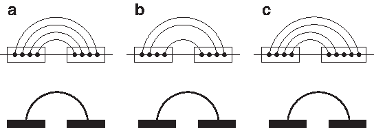
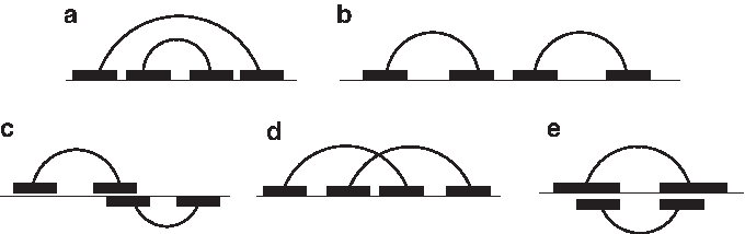
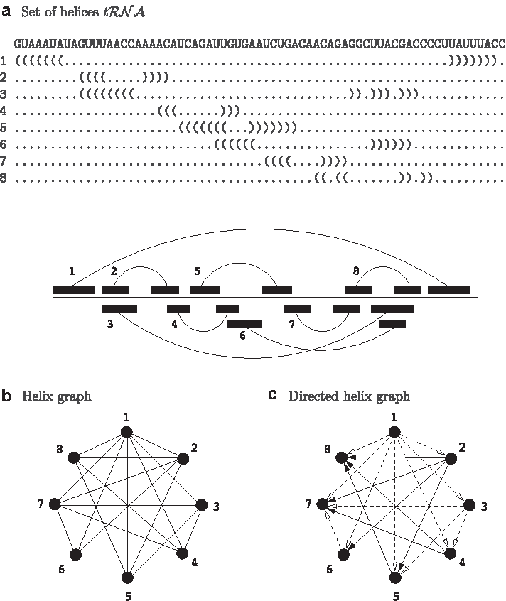
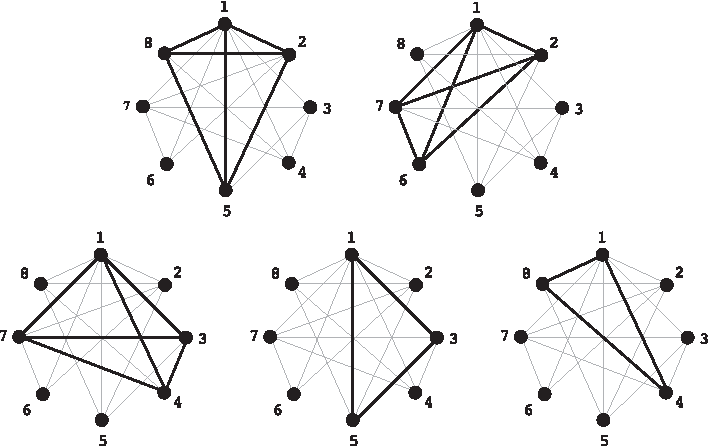

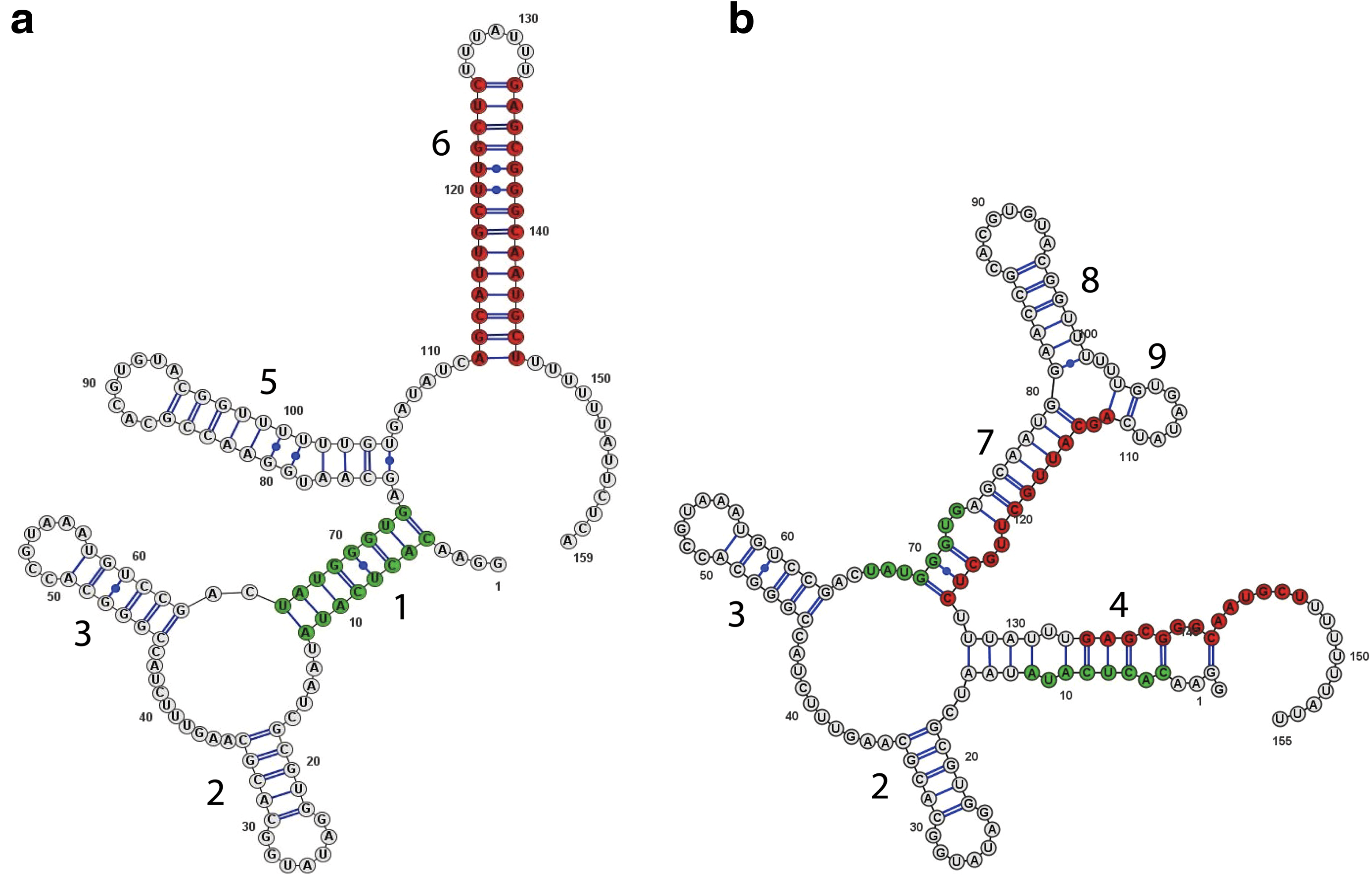
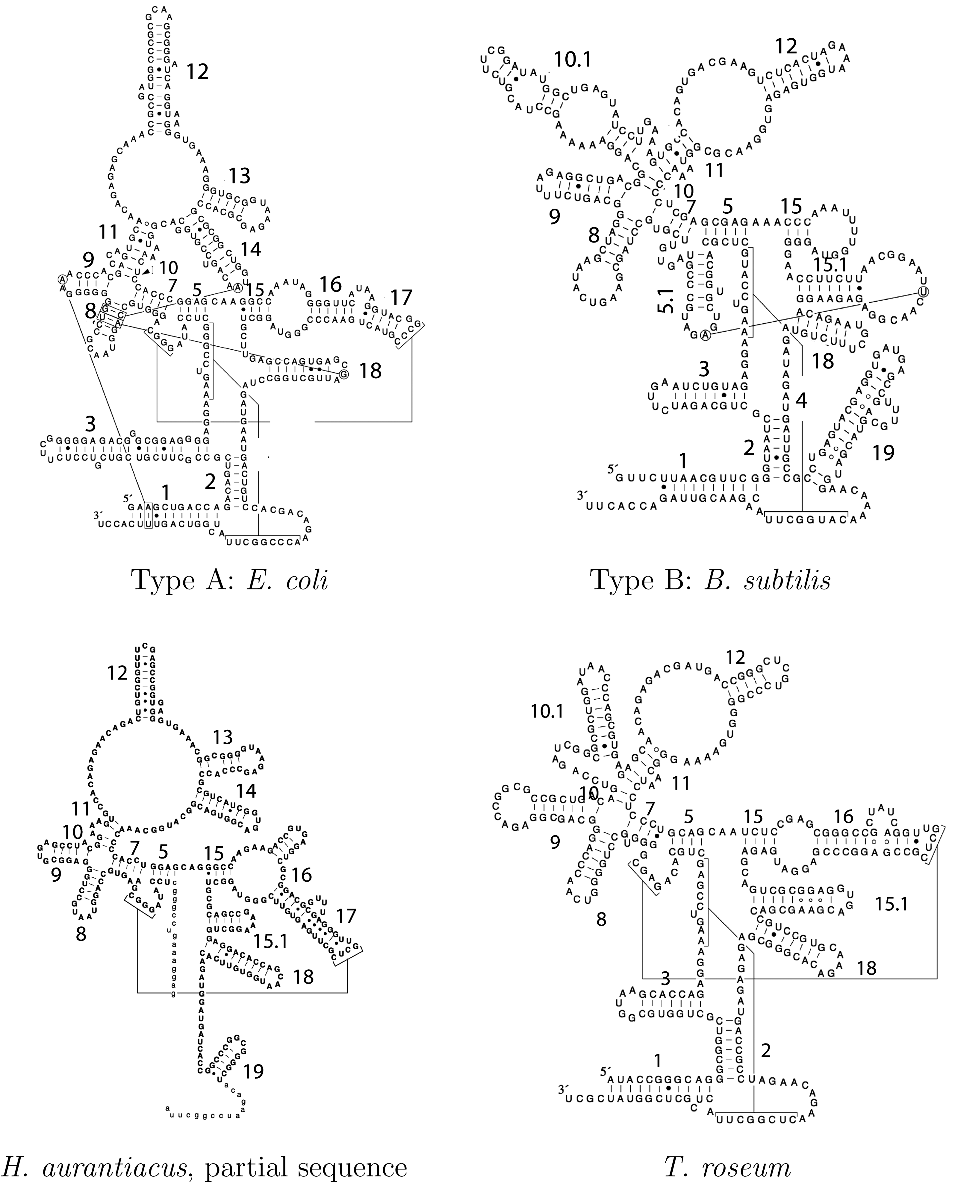


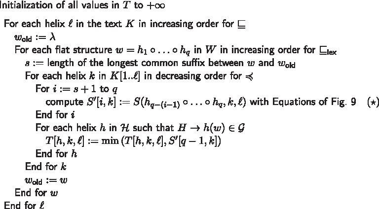
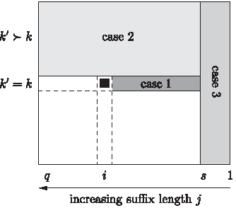
 operators in Equation (⋄) and in the caption of Figure 9 have to be replaced by max operators when computing T and