Learning Sequence Determinants of Protein:Protein Interaction Specificity with Sparse Graphical Models

Abstract

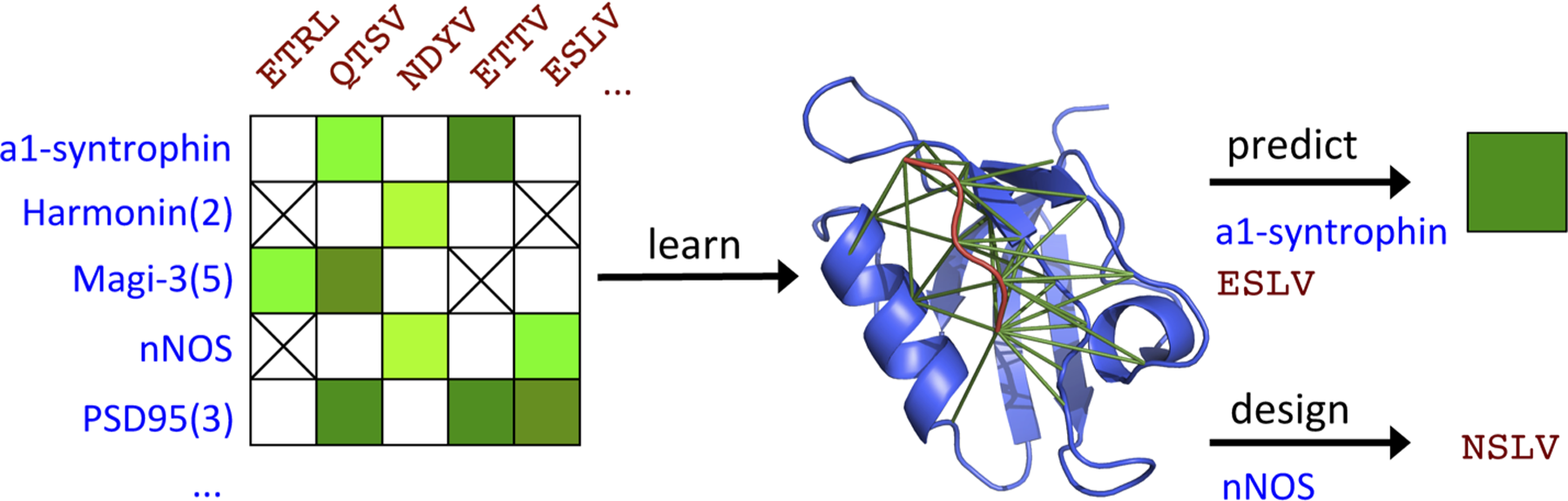
In studying the strength and specificity of interaction between members of two protein families, key questions center on which pairs of possible partners actually interact, how well they interact, and why they interact while others do not. The advent of large-scale experimental studies of interactions between members of a target family and a diverse set of possible interaction partners offers the opportunity to address these questions. We develop here a method, DgSpi (data-driven graphical models of specificity in protein:protein interactions), for learning and using graphical models that explicitly represent the amino acid basis for interaction specificity (why) and extend earlier classification-oriented approaches (which) to predict the ΔG of binding (how well). We demonstrate the effectiveness of our approach in analyzing and predicting interactions between a set of 82 PDZ recognition modules against a panel of 217 possible peptide partners, based on data from MacBeath and colleagues. Our predicted ΔG values are highly predictive of the experimentally measured ones, reaching correlation coefficients of 0.69 in 10-fold cross-validation and 0.63 in leave-one-PDZ-out cross-validation. Furthermore, the model serves as a compact representation of amino acid constraints underlying the interactions, enabling protein-level ΔG predictions to be naturally understood in terms of residue-level constraints. Finally, the model DgSpi readily enables the design of new interacting partners, and we demonstrate that designed ligands are novel and diverse.

1. Introduction

The molecular machinery of the cell is driven largely by protein:protein interactions. Traditional high-throughput technologies (Fields and Song, 1989) provide evidence for the existence of interactions that existing computational systems biology techniques utilize to build global networks of interacting proteins. However, finer-grained methods are necessary in order to better understand, predict, and control these interactions. Fortunately, appropriate experimental methodologies are rapidly developing, for example, using protein microarrays to isolate numerous pairs of possible partners, and fluorescence polarization to assess their interaction strength (Fig. 1, left). Several large-scale studies have been conducted using such techniques for particular families of interacting proteins, including PDZ domains and their peptide ligands (Chen et al., 2008; Tonikian et al., 2008), and human basic-region leucine zippers (bZIPs) and their coiled-coil partners (Fong et al., 2004; Grigoryan et al., 2009). In lieu of large-scale studies, the aggregation of a large number of smaller-scale experiments can also yield extensive amounts of detailed binding data, for example, for major histocompability complex (MHC) and ligands (Peters et al., 2005; Nielsen et al., 2007; Wang et al., 2008; Bordner and Mittelmann, 2010; Zhang et al., 2012), and serine proteases and inhibitors (Lu et al., 2001; Li et al., 2005).

FIG. 1.

Data-driven Graphical models of Specificity in Protein:protein Interactions (DgSpi). A graphic model of PDZ:peptide interactions encapsulates the amino acid constraints conferring the strength and specificity of the interactions in an input dataset. (Left) The dataset has ΔG values (shades of green) or “noninteracting” indications (X's) for some PDZ (blue)–peptide (red) pairs. (Middle) We learn a graphical model with bipartite nodes for some residues in the PDZ (blue) and peptide (red), with edges (green) encapsulating and providing a probabilistic interpretation for amino acid constraints. (Right) We use the model to predict novel interactions as well as to design novel peptide partners for PDZs.

As one particular example, consider the specific recognition between PDZ domains and their peptide ligands. PDZs are small peptide recognition modules that bind specific C-terminal peptides of other proteins (Fig. 1, right), in order to mediate protein:protein interactions (e.g., in signaling networks). Early studies of PDZ:peptide recognition developed consensus motifs to capture the common amino acids comprising the ligands of different PDZ “classes” (e.g., class I = S/T-X-Φ vs. class II = Φ-X-Φ, where Φ is a hydrophobic residue). More recent studies yielded more refined statistical binary interaction predictors (interact or not?), based on analysis of amino acid pairs (across the PDZ:peptide interface) in curated datasets of experimentally identified PDZ:ligand partners (Brannetti et al., 2000; Thomas et al., 2009a). MacBeath and colleagues then made the leap to large-scale quantitative data, determining the ΔG of binding for 829 PDZ:peptide pairs from 96 PDZs (from mouse, fly, and worm) against a panel of 259 possible peptide partners in Stiffler et al. (2007). They used this data to develop a binary interaction predictor, based on the constituent PDZ:peptide amino acid pairs like the predictors mentioned above, but taking advantage of the quantitative and negative data in Chen et al. (2008). More recently, Bader and coworkers used the MacBeath data to train a type of support vector regression model for predicting ΔG of binding for PDZ:peptide pairs in Shao et al. (2010).

Motivated by the exciting growth in quantitative studies of protein:protein interactions, we have developed a data-driven, sequence-based model that directly and compactly reveals and represents the amino acid interactions underlying experimentally measured ΔG values of binding (henceforth just ΔG) and enables efficient, accurate, robust, and transparent prediction of ΔGs for new pairs of possible partners (Fig. 1). We employ a graph-structured model (which we refer to simply as a graphical model) that explicitly models amino acid interactions and provides a probabilistic interpretation for them. Sequence-based graphical models of protein families have been used to capture amino acid interactions in order to predict protein structure (Morcos et al., 2011; Jones et al., 2012; Kamisetty et al., 2013) and function (Thomas et al., 2008; Balakrishnan et al., 2011) and design new proteins (Thomas et al., 2009b; Kamisetty et al., 2011b). We build here on our sequence-based models of interacting protein families for binary prediction of interaction developed in Thomas et al. (2009a), significantly extending that approach to incorporate quantitative data and thereby predict ΔG.

We call our approach DgSpi, for data-driven graphical models of specificity in protein:protein interactions. Using the PDZ data from MacBeath and coworkers, we demonstrate that DgSpi is highly predictive of ΔG, obtaining predicted-experimental correlation coefficients of up to 0.69 in a ten-fold cross-validation and 0.63 in leave-one-PDZ-out cross-validation. This performance is essentially equivalent to that obtained by Shao et al. (2010), but importantly, our approach provides a readily interpretable model of the amino acid contributions underlying specific interactions. Furthermore, since our graphical models can be used in designing new interacting partners (again, interpretable in terms of the amino acid contributions), and we show that there is a diversity of novel peptides that are predicted to bind well against any given PDZ and thus provide worthwhile hypotheses for experimental testing.

2. Methods

DgSpi takes as input (Fig. 1, left) two sets of protein sequences; for simplicity but without implications about function, we refer to one set as the “receptor” and the other as the “ligand”; for example, the PDZ protein recognition modules as receptors and corresponding peptides as ligands. In addition to the sequences, there are experimental binding measurements for some of the pairs (one from each set); the measurement is either a ΔG value or an indication of “noninteracting” within the sensitivity of the experiment. Our goal is to be able to predict the ΔG of interaction for a previously untested receptor:ligand pair and to design new ligand partners for a specified receptor (Fig. 1, right). To do this, we seek a method that admits explanation of predictions in terms of the underlying amino acid-level interactions conferring specificity of interaction. Thus we employ a graph-structured, or graphical, model (Fig. 1, middle) with nodes for the receptor and ligand residues, and bipartite edges capturing the amino acid constraints between receptor and ligand residues. We first summarize a graphical model to predict ΔG from a pair of sequences, and then the algorithms to construct a model from training data of sequence pairs with observed ΔG.

2.1. A graphical model of binding free energy

We assume the receptors have been multiply aligned to p informative (nongappy) columns, and the ligands likewise to q residues. Let \documentclass{aastex}\usepackage{amsbsy}\usepackage{amsfonts}\usepackage{amssymb}\usepackage{bm}\usepackage{mathrsfs}\usepackage{pifont}\usepackage{stmaryrd}\usepackage{textcomp}\usepackage{portland, xspace}\usepackage{amsmath, amsxtra}\pagestyle{empty}\DeclareMathSizes{10}{9}{7}{6}\begin{document} $${ \bf X} = \{ X_{1} , X_{2} , \ldots , X_{p} \} $$ \end{document} be a set of p random variables representing the receptor amino acid composition, with X_i a discrete random variable for the amino acid type at position i. Each X_i takes values in \documentclass{aastex}\usepackage{amsbsy}\usepackage{amsfonts}\usepackage{amssymb}\usepackage{bm}\usepackage{mathrsfs}\usepackage{pifont}\usepackage{stmaryrd}\usepackage{textcomp}\usepackage{portland, xspace}\usepackage{amsmath, amsxtra}\pagestyle{empty}\DeclareMathSizes{10}{9}{7}{6}\begin{document} $${ \cal A} = \{ ala , arg , \ldots , val , - \} $$ \end{document} , corresponding to the 20 amino acid types and an additional “-” for a gap in the multiple sequence alignment. Similarly, let \documentclass{aastex}\usepackage{amsbsy}\usepackage{amsfonts}\usepackage{amssymb}\usepackage{bm}\usepackage{mathrsfs}\usepackage{pifont}\usepackage{stmaryrd}\usepackage{textcomp}\usepackage{portland, xspace}\usepackage{amsmath, amsxtra}\pagestyle{empty}\DeclareMathSizes{10}{9}{7}{6}\begin{document} $${ \bf Y} = \{ Y_{1} , Y_{2} , \ldots , Y_{q} \} $$ \end{document} be a set of q random variables representing the ligand composition.

Given a receptor sequence \documentclass{aastex}\usepackage{amsbsy}\usepackage{amsfonts}\usepackage{amssymb}\usepackage{bm}\usepackage{mathrsfs}\usepackage{pifont}\usepackage{stmaryrd}\usepackage{textcomp}\usepackage{portland, xspace}\usepackage{amsmath, amsxtra}\pagestyle{empty}\DeclareMathSizes{10}{9}{7}{6}\begin{document} $${ \bf x} = \{ x_1 , x_2 , \ldots , x_p \} $$ \end{document} (i.e., amino acid values for the random variables in X), along with a ligand sequence \documentclass{aastex}\usepackage{amsbsy}\usepackage{amsfonts}\usepackage{amssymb}\usepackage{bm}\usepackage{mathrsfs}\usepackage{pifont}\usepackage{stmaryrd}\usepackage{textcomp}\usepackage{portland, xspace}\usepackage{amsmath, amsxtra}\pagestyle{empty}\DeclareMathSizes{10}{9}{7}{6}\begin{document} $${ \bf y} = \{ y_1 , y_2 , \ldots , y_q \} $$ \end{document} , we want to predict the strength of a possible interaction between the two proteins, ΔG_pred(x, y). Our goal here is to develop a robust predictive model that is interpretable in terms of the amino acid interactions driving specific protein:protein recognition. Therefore, we model ΔGpred with a bipartite graphical model, with nodes for X and Y representing the amino acids and edges \documentclass{aastex}\usepackage{amsbsy}\usepackage{amsfonts}\usepackage{amssymb}\usepackage{bm}\usepackage{mathrsfs}\usepackage{pifont}\usepackage{stmaryrd}\usepackage{textcomp}\usepackage{portland, xspace}\usepackage{amsmath, amsxtra}\pagestyle{empty}\DeclareMathSizes{10}{9}{7}{6}\begin{document} $${ \cal E} \subset { \bf X} \times { \bf Y}$$ \end{document} representing their dependencies. Nodes x_i, y_j have associated \documentclass{aastex}\usepackage{amsbsy}\usepackage{amsfonts}\usepackage{amssymb}\usepackage{bm}\usepackage{mathrsfs}\usepackage{pifont}\usepackage{stmaryrd}\usepackage{textcomp}\usepackage{portland, xspace}\usepackage{amsmath, amsxtra}\pagestyle{empty}\DeclareMathSizes{10}{9}{7}{6}\begin{document} $$\mid { \cal A} \mid \times 1$$ \end{document} vectors V_i[a], V_j[b] to capture position-specific environment effects to binding. Edge (i, j), between nodes x_i and y_j, has an associated \documentclass{aastex}\usepackage{amsbsy}\usepackage{amsfonts}\usepackage{amssymb}\usepackage{bm}\usepackage{mathrsfs}\usepackage{pifont}\usepackage{stmaryrd}\usepackage{textcomp}\usepackage{portland, xspace}\usepackage{amsmath, amsxtra}\pagestyle{empty}\DeclareMathSizes{10}{9}{7}{6}\begin{document} $$\mid { \cal A} \mid \times \mid { \cal A} \mid$$ \end{document} matrix W_i,j[a, b] of weights for \documentclass{aastex}\usepackage{amsbsy}\usepackage{amsfonts}\usepackage{amssymb}\usepackage{bm}\usepackage{mathrsfs}\usepackage{pifont}\usepackage{stmaryrd}\usepackage{textcomp}\usepackage{portland, xspace}\usepackage{amsmath, amsxtra}\pagestyle{empty}\DeclareMathSizes{10}{9}{7}{6}\begin{document} $$a , b \in { \cal A}$$ \end{document} , holding the position-specific contributions to binding for each possible pair of amino acids, intended to capture electrostatics, van der Waals, hydrogen bonding, and other such interactions, which depend on the composition of the amino acids involved. We point out that these physical justifications for the parameters of our model are descriptive rather than prescriptive: they guide the intuition for learning and interpreting the model, but we make no assumptions on sources of these interactions beyond what we can learn from data.

In summary, then, given two protein sequences x and y, we predict their binding free energy as: \documentclass{aastex}\usepackage{amsbsy}\usepackage{amsfonts}\usepackage{amssymb}\usepackage{bm}\usepackage{mathrsfs}\usepackage{pifont}\usepackage{stmaryrd}\usepackage{textcomp}\usepackage{portland, xspace}\usepackage{amsmath, amsxtra}\pagestyle{empty}\DeclareMathSizes{10}{9}{7}{6}\begin{document} \begin{align*}\Delta G_{pred} ( { \bf x , y} ) = \mathop \sum \limits_{i = 1}^{p} V_{i} [ x_i ] + \mathop \sum \limits_{j = 1}^{q} V_{j} [ y_j ] + \sum_{ ( i , j ) \in { \cal E}} W_{i , j} [ x_i , y_j ] \tag{1}\end{align*} \end{document}

2.2. Training objective

Our data-driven approach to modeling protein:protein interaction specificity uses experimental data to learn the parameters V and W that define the model in Equation 1. We assume that the experimental data is partitioned into interactions \documentclass{aastex}\usepackage{amsbsy}\usepackage{amsfonts}\usepackage{amssymb}\usepackage{bm}\usepackage{mathrsfs}\usepackage{pifont}\usepackage{stmaryrd}\usepackage{textcomp}\usepackage{portland, xspace}\usepackage{amsmath, amsxtra}\pagestyle{empty}\DeclareMathSizes{10}{9}{7}{6}\begin{document} $${ \cal I}_{+}$$ \end{document} , with ΔG values, and noninteractions \documentclass{aastex}\usepackage{amsbsy}\usepackage{amsfonts}\usepackage{amssymb}\usepackage{bm}\usepackage{mathrsfs}\usepackage{pifont}\usepackage{stmaryrd}\usepackage{textcomp}\usepackage{portland, xspace}\usepackage{amsmath, amsxtra}\pagestyle{empty}\DeclareMathSizes{10}{9}{7}{6}\begin{document} $${ \cal I}_{-}$$ \end{document} , where the binding was weaker than ΔGmax, a maximum experimentally detectable ΔG value. Thus each member of \documentclass{aastex}\usepackage{amsbsy}\usepackage{amsfonts}\usepackage{amssymb}\usepackage{bm}\usepackage{mathrsfs}\usepackage{pifont}\usepackage{stmaryrd}\usepackage{textcomp}\usepackage{portland, xspace}\usepackage{amsmath, amsxtra}\pagestyle{empty}\DeclareMathSizes{10}{9}{7}{6}\begin{document} $${ \cal I}_{+}$$ \end{document} is of the form (x, y, ΔG), giving a pair of sequences and the measured ΔG value, while each member of \documentclass{aastex}\usepackage{amsbsy}\usepackage{amsfonts}\usepackage{amssymb}\usepackage{bm}\usepackage{mathrsfs}\usepackage{pifont}\usepackage{stmaryrd}\usepackage{textcomp}\usepackage{portland, xspace}\usepackage{amsmath, amsxtra}\pagestyle{empty}\DeclareMathSizes{10}{9}{7}{6}\begin{document} $${ \cal I}_{-}$$ \end{document} is simply an (x, y) pair.

We take as our primary objective minimizing the squared error between the observed and predicted ΔG values for members of \documentclass{aastex}\usepackage{amsbsy}\usepackage{amsfonts}\usepackage{amssymb}\usepackage{bm}\usepackage{mathrsfs}\usepackage{pifont}\usepackage{stmaryrd}\usepackage{textcomp}\usepackage{portland, xspace}\usepackage{amsmath, amsxtra}\pagestyle{empty}\DeclareMathSizes{10}{9}{7}{6}\begin{document} $${ \cal I}_{+}$$ \end{document} . For the noninteractions in \documentclass{aastex}\usepackage{amsbsy}\usepackage{amsfonts}\usepackage{amssymb}\usepackage{bm}\usepackage{mathrsfs}\usepackage{pifont}\usepackage{stmaryrd}\usepackage{textcomp}\usepackage{portland, xspace}\usepackage{amsmath, amsxtra}\pagestyle{empty}\DeclareMathSizes{10}{9}{7}{6}\begin{document} $${ \cal I}_{-}$$ \end{document} , we incorporate a penalty for an incorrect prediction, that is, for ΔG_pred better than ΔG_max. In particular, we use a one-sided squared penalty for noninteractions predicted as interactions. Compared with the hinge-loss commonly used in SVMs, this tends to penalize small differences to a lesser extent, which is a desirable property in cases such as ours where the focus is on the regression error and not the misclassification cost. The one-sided square error has no points of discontinuity, making optimization easier as well.

Thus our objective function for a specific set of parameters V, W is: \documentclass{aastex}\usepackage{amsbsy}\usepackage{amsfonts}\usepackage{amssymb}\usepackage{bm}\usepackage{mathrsfs}\usepackage{pifont}\usepackage{stmaryrd}\usepackage{textcomp}\usepackage{portland, xspace}\usepackage{amsmath, amsxtra}\pagestyle{empty}\DeclareMathSizes{10}{9}{7}{6}\begin{document} \begin{align*} \begin{split}L ( V , W ) & = \sum_{ ( { \bf x , y , } \Delta G ) \in { \cal I}_{+} } ( \Delta G_{pred} ( { \bf x , y};V , W ) - \Delta G ) ^2 \\ & + \sum_{ ( { \bf x , y} ) \in { \cal I}_{ -}\,{ s.t.} \atop \Delta G_{pred} ( { \bf x , y};V , W ) < \Delta G_{max}} \gamma_{-} \cdot ( \Delta G_{pred} ( { \bf x , y};V , W ) - \Delta G_{max} ) ^2\end{split} \tag{2}\end{align*} \end{document}

where we emphasize the dependence of ΔG_pred in Equation 1 on V and W by including them as parameters. The parameter γ_- sets the relative weighting between the contributions from interactions and non-interactions.

2.3. Block-sparse regularization

A suitable model can be learned from the data by minimizing the objective function in Equation 2. However, directly optimizing this function is likely to lead in overfitting as there are usually far more parameters in the model than there are data points available with which to fit them. To circumvent this problem, we instead optimize a regularized objective function. Regularization is usually described as a penalty to the objective function; an alternate but equivalent view of the regularization is that it is a Bayesian prior on the models that biases the learning method toward models consistent with the prior. Protein:protein interactions can be reasonably expected to display structural sparsity—due to spatial restrictions, only a few of all possible bipartite interactions between the partners are likely to be important in biochemical interactions. Motivated by this prior belief, we employ block-L1 regularization, a form of regularization that penalizes the number of nonzero edges (or “blocks”), so that each edge (i, j) is penalized unless all parameters within the edge, W_i,j, are zero. This promotes a sparser structure promoting interpretability; furthermore, by reducing the number of nonzero parameters in the model, it helps avoid overfitting. For our model, the block-L1 regularization term is: \documentclass{aastex}\usepackage{amsbsy}\usepackage{amsfonts}\usepackage{amssymb}\usepackage{bm}\usepackage{mathrsfs}\usepackage{pifont}\usepackage{stmaryrd}\usepackage{textcomp}\usepackage{portland, xspace}\usepackage{amsmath, amsxtra}\pagestyle{empty}\DeclareMathSizes{10}{9}{7}{6}\begin{document} \begin{align*}R_ { 1 , 2 } ( V , W ) = \frac { 1 } { \sqrt { \mid { \cal A } \mid } } \left( \mathop \sum \limits_ { i = 1 } ^ { p } \parallel V_i \parallel + \mathop \sum \limits_ { j = 1 } ^ { q } \parallel V_j \parallel \right) + \sum_ { ( i , j ) \in { \cal E } } \parallel W_ { i , j } \parallel \tag { 3 } \end{align*} \end{document}

where ∥·∥ refers to the vector two-norm of the corresponding set of parameters and the fraction \documentclass{aastex}\usepackage{amsbsy}\usepackage{amsfonts}\usepackage{amssymb}\usepackage{bm}\usepackage{mathrsfs}\usepackage{pifont}\usepackage{stmaryrd}\usepackage{textcomp}\usepackage{portland, xspace}\usepackage{amsmath, amsxtra}\pagestyle{empty}\DeclareMathSizes{10}{9}{7}{6}\begin{document} $$ \frac { 1 } { \sqrt { \mid { \cal A } \mid } } $$ \end{document} (number of amino acids plus gap) is a correction factor to account for the different degrees of freedom in V and W.

Our learning objective is then: \documentclass{aastex}\usepackage{amsbsy}\usepackage{amsfonts}\usepackage{amssymb}\usepackage{bm}\usepackage{mathrsfs}\usepackage{pifont}\usepackage{stmaryrd}\usepackage{textcomp}\usepackage{portland, xspace}\usepackage{amsmath, amsxtra}\pagestyle{empty}\DeclareMathSizes{10}{9}{7}{6}\begin{document} \begin{align*}\arg \min_{V , W}\, \left( L ( V , W ) + \lambda_{1 , 2} \cdot R_{1 , 2} ( V , W ) \right) \tag{4}\end{align*} \end{document}

where λ_1,2 sets the relative weight between the learning objective and the regularization term.

2.4. Learning algorithms

Schmidt et al. (2009) developed a limited-memory projected quasi-newton (PQN) approach suitable for squared error objectives. We customize their method for our graphical models of protein–protein interactions. A constrained optimization to incorporate the block-L1 regularization is performed by a projected gradient method that iterates between unconstrained gradient descent updates to the parameter values, and constrained projections of the parameter values onto the constrained space.

While this approach can be used to learn the structure and parameters of the model (i.e., which vertices and edges, along with their weights), in practice, the resulting procedure can result in biased weights for the nonzero parameters, despite identifying the correct structure (Meinshausen and Bühlmann, 2006; Balakrishnan et al., 2011). To avoid this, after learning the structure of the model, we relearn the nonzero parameters with L2 regularization. That is, in a second stage, we restrict the optimization to the vertices and edges contributing in the first stage, but reoptimize their weights using a modified version of Equation 4, replacing R_1,2 with: \documentclass{aastex}\usepackage{amsbsy}\usepackage{amsfonts}\usepackage{amssymb}\usepackage{bm}\usepackage{mathrsfs}\usepackage{pifont}\usepackage{stmaryrd}\usepackage{textcomp}\usepackage{portland, xspace}\usepackage{amsmath, amsxtra}\pagestyle{empty}\DeclareMathSizes{10}{9}{7}{6}\begin{document} \begin{align*}R_2 ( V , W ) = \mathop \sum \limits_{i = 1}^{p} \parallel V_i \parallel^{2} + \mathop \sum \limits_{j = 1}^{q} \parallel V_j \parallel^{2} + \sum_{ ( i , j ) \in { \cal E}} \parallel W_{i , j} \parallel^{2} , \tag{5}\end{align*} \end{document}

weighted by a corresponding λ₂. Since R₂(V, W) penalizes the square of the vector 2-norms, each element of each parameter vector is penalized independent of any group membership; the regularization is thus independent of the degrees of freedom in the corresponding groups. This two-stage approach finds sparse models with small edge weights, regularizing a pseudo-likelihood objective similarly to the approach of Balakrishnan et al. (2011). We find in practice that this approach yields models that are both interpretable and predictive of ΔG.

3. Results

Our goal is to make quantitative predictions of the ΔG of PDZ:peptide interactions, interpretable in terms of underlying amino acid constraints. This is in contrast to the approach of Chen et al. (2008), who studied the ability of a computational method to classify interaction vs. noninteraction. [A graphical model approach to do that has been previously described in Thomas et al. (2009a); we have found that classifying based on predicted ΔG is not as robust.] It is also in contrast to the support vector regression approach of Shao et al. (2010), in that while our method achieves comparable predictive accuracy, it has the added benefit of being able to automatically identify the amino acid-level interactions with the greatest impact, and directly characterize their contributions. These interactions not only allow us to characterize the sequence determinants of binding affinity and specificity, but also allow us to design new interacting partners based on the derived “rules” of good interactions.

We apply DgSpi to the extensive PDZ dataset collected by Stiffler et al. (2007) and Chen et al. (2008). To enable appropriate comparison of results, we use the processed version of the dataset provided by Shao et al. (2010). The dataset includes 82 mouse PDZs and 217 peptides, with a reported 560 interactions and 1167 noninteractions. We obtained a structure- and sequence-based multiple sequence alignment of 225 columns where the peptides were represented by five C-terminal residues. We then removed highly conserved and highly gap-ful columns, reducing the alignment to 114 PDZ positions and 5 peptide positions.

3.1. ΔG prediction

3.1.1. 10-fold cross-validation

To test the ability of our model to predict the affinity of PDZ-peptide interaction, we first performed a ten-fold cross-validation (i.e., we learned the model with 90% of the data and tested it on the left-out 10%, doing this with each 10% left out). This represents the scenario in which data are available for some interactions, and we want to make predictions for others.

Our learning approach has three main parameters: γ₋, a parameter trading off the relative importance of positive and negative interactions in the objective function; λ_1,2, the strength of the block-L1 regularization used to determine the nonzero parameters of the model, and λ₂, the regularization weight used to estimate the values of the nonzero parameters. The γ₋ and λ₂ were set to 0.05 and 1, respectively, based on our initial experiments using one train-test split. The small value of γ₋ reflects the relative abundance of noninteractions in our dataset and our emphasis on modeling interactions comprehensively since they are biologically more interesting. For each training split, we varied λ_1,2 generating multiple models spanning the spectrum from models with no interactions to models where nearly all possible interactions were allowed.

Figure 2 summarizes trends over values of λ_1,2. The top panel characterizes the increase in number of interactions with decreasing λ_1,2, and the middle panel the corresponding increase in the average Pearson correlation coefficient, from 0.49 when there are no edges in the model and all contributions are due to the V_i, V_j, to 0.66 when ∼60 interactions are included, to a maximum of 0.69 when ∼300 interactions are included. The relatively large increase in model accuracy when the number of edges increases from 0 to 60 suggests that these edges make important contributions to binding affinity and specificity. In contrast, the relatively small increase in accuracy of the model as the number of edges increases beyond 60 to being a completely connected model suggests that the edges introduced later have relatively low importance. The bottom panel shows the average strength of each edge, calculated as the norm of W_i,j, as a function of λ_1,2. Each line represents a separate unique interacting pair of residues; interactions that have high weight at λ=25 are highlighted in color, while the remaining interactions are shown in black. When the model is sparse (high λ_1,2), there are few, strong interactions; as the density of the model increases (low λ_1,2), most interactions have nonzero strength but are very weak.

FIG. 2.

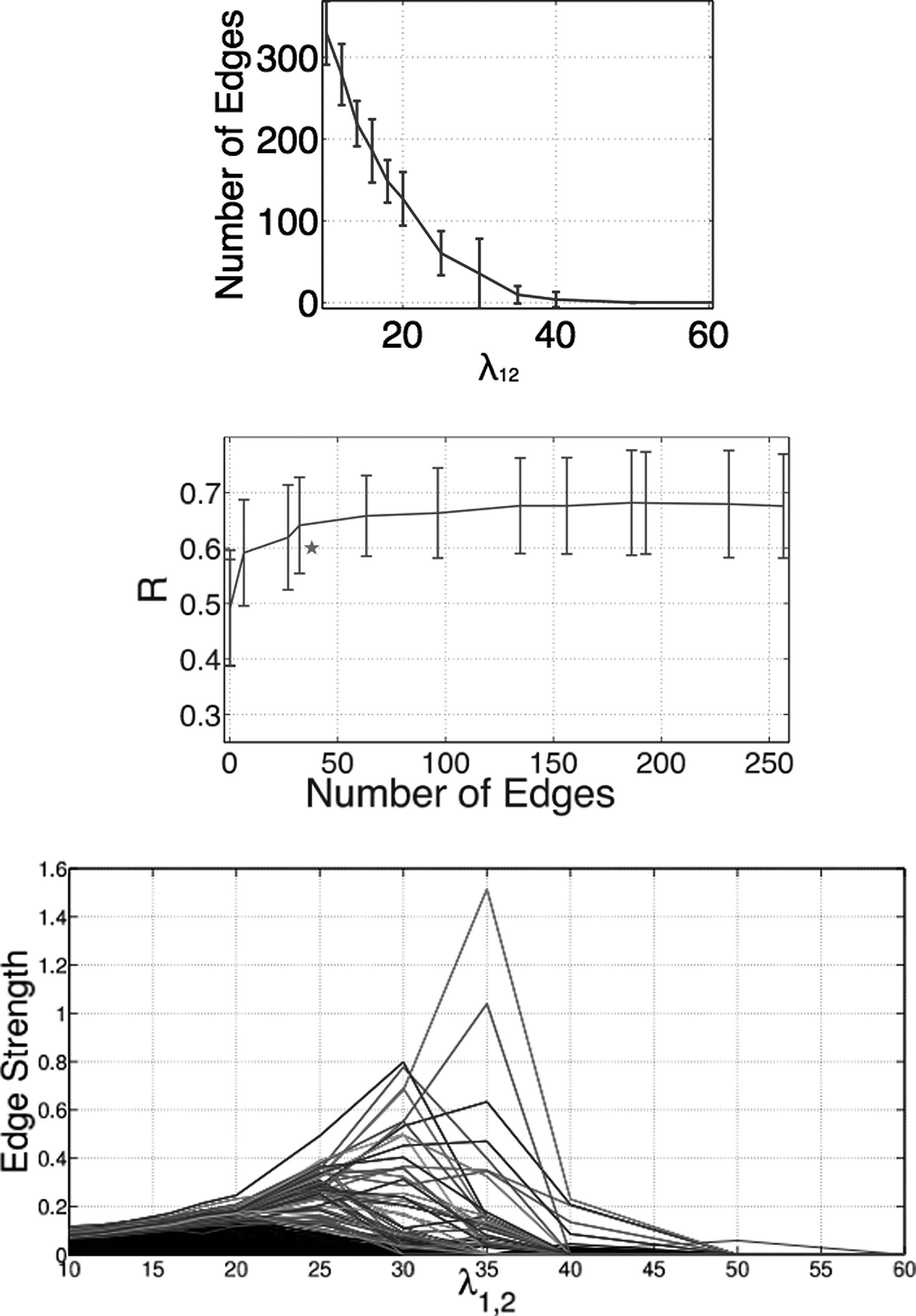
Trends with varying regularization weight (parameter λ_1,2), with higher values yielding sparser models. (Top) Number of edges in models learned with varying λ_1,2. (Middle) Regularization path, showing each edge's strength as a function of λ_1,2. The star indicates a model with edges fixed according to contacts in a crystal structure. (Bottom) Test correlation coefficient as a function of the average number of edges in trained model.

Figure 3 shows the prediction results for one 10-fold repetition at λ_1,2=20. The overall correlation coefficient across the dataset was 0.67 while the root mean square error between experiment and prediction was 0.62. Most errors were equally distributed around zero, and actually within typical experimental error. However, there were a few clear outliers where the model under-predicted binding energies.

FIG. 3.

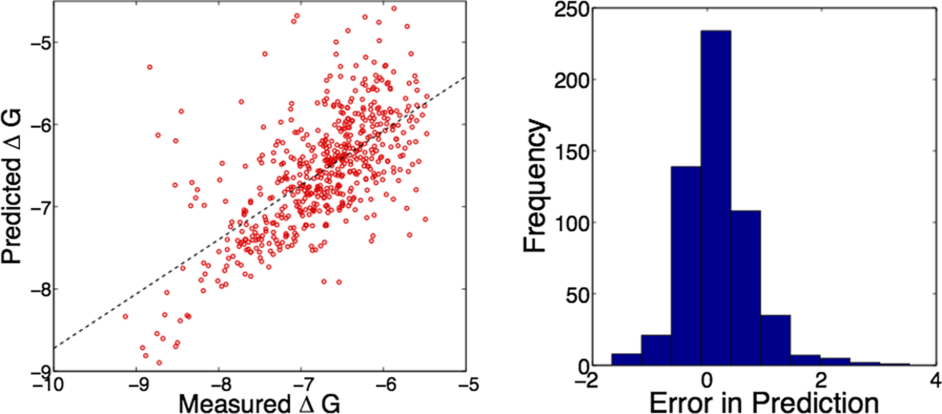
Example prediction results, combined across 10 splits in one repetition at λ_1,2 = 20. (Left) Scatterplots of experimental vs. predicted ΔG. Pearson correlation coefficient across entire test-split was 0.67. (Right) Histogram of prediction errors.

3.1.2. Contact-based model structure

When an experimentally determined 3D structure of the protein–protein interface is available, an alternate approach to determining the structure (edges) of the graphical model could be to restrict the nonzero interactions to the pairs of residues close to each other in the 3D structure. The parameters of this model with fixed structure can then be readily learned with L2 regularization, as before. Chen et al. (2008) identified 38 contacts between 16 PDZ residues and 5 peptides. We repeated our 10-fold cross-validation experiments, using these 21 positions and 38 contacting residues as the set of vertices and edges in the model (instead of identifying them using the block-L1 penalty), and estimated their parameters with L2 regularization. The average correlation coefficient of the contact-based models is 0.60, which, while good, is lower than the 0.66 correlation obtained by models with about 60 interactions. Could the difference in accuracy be due to the difference in the number of interactions? The middle panel in Figure 2 highlights the accuracy of this model (shown as a star), compared to the correlation coefficients obtained by varying λ_1,2. We see that the models with learned structure can achieve accuracy similar to the contact-structure model but using fewer interactions; alternativeely, a model with learned structure and a comparable number of interactions to that of the contact structure achieves higher correlation. Thus, our data-driven approach to learning model structure can identify important interactions beyond those that might be inferred by inspection of the 3D structure.

3.1.3. Leave-one PDZ out

To test the scenario where the model is applied to make predictions for a new PDZ, we performed “leave-one-PDZ-out” cross-validation following the approach of Shao et al. (2010). We held out data for each of the 23 PDZ domains with at least 10 interactions, training the model on the remaining data and testing on the held-out domain. Since the effect of λ_1,2 on the sparsity of the model depends on the number of sequences in the training set, instead of choosing the same value of as selected by ten-fold cross-validation, we performed a grid search on λ_1,2 and used the value that gives a model of similar sparsity as the cross-validated models. This process allows us to parameterize the model by the number of edges as opposed to the less natural λ_1,2. Using this procedure we obtained an average correlation coefficient of 0.61 across the 23 PDZs that had at least 10 interactions. Again, allowing for denser models by changing the regularization weight slightly improved the average correlation coefficient to 0.63, which is comparable to the 0.65 obtained by Shao et al. (2010) using support vector regression. Table 1 summarizes the correlation coefficient by domain. When restricting to contact edges, we obtain 0.54, about the same as the 0.56 of Bader and colleagues (domain-level details not shown).

Table 1.

Leave-One-PDZ-Out Cross-Validation

PDZ sequence	DgSpi-dense	DgSpi-sparse	SemiSVR
CHAPSYN-110-2/3	0.91	0.93	0.94
CHAPSYN-110-3/3	0.68	0.67	0.88
GM1582-2/3	0.61	0.69	0.58
G1-SYNTROPHIN-1/1	0.22	0.16	0.13
HTRA3-1/1	0.60	0.53	0.65
LIN7C-1/1	0.61	0.61	0.68
MAGI-2-2/6	0.73	0.73	0.77
MAGI-2-6/6	0.77	0.84	0.69
MAGI-3-1/5	0.77	0.80	0.88
MALS2-1/1	0.32	0.37	0.61
OMP25-1/1	0.61	0.56	0.50
PDZK3-1/1	0.06	0.07	0.04
PDZ-RGS3-1/1	0.14	0.16	0.03
PSD95-2/3	0.91	0.91	0.92
PSD95-3/3	0.86	0.90	0.88
PTP-BL-2/5	0.35	0.41	0.40
SAP97-1/3	0.68	0.70	0.76
SAP97-2/3	0.96	0.95	0.95
SAP102-2/3	0.94	0.95	0.94
SCRB1-3/4	0.76	0.82	0.69
SHANK1-1/1	0.83	0.92	0.98
SHANK3-1/1	0.67	0.68	0.51
ZO-1-1/3	0.01	0.09	0.65
Average	0.63	0.61	0.65

Leave-one-PDZ-out cross-validation following Bader and colleagues (Shao et al., 2010) with the published performance of their method (their Table 3) reproduced in the “SemiSVR” column.

3.2. Model analysis

A key feature of DgSpi is that a model can be easily “opened up” to characterize the amino acid determinants of binding. To illustrate, we characterized the models trained at λ_1,2=25 across the 10 folds, computing the average strength of the vector 2-norms for the protein positions (i.e., V_i), peptide positions (i.e., V_j), and potentially interacting pairs (i.e., W_i,j). Figure 4 (top) shows these values: The strengths of the vertex terms appear along the axes (x-axis for PDZ positions and y-axis for peptide positions), while the strengths of the PDZ:peptide edge terms appear in the heat map. As might be expected for interaction affinities, the position-based terms are relatively weaker, with most being less than 0.2. In contrast, more than 40 interaction terms have norms larger than this value, with a large fraction of them between position 4 of the peptide and the protein. Figure 4 (bottom left) overlays these strong interactions on the structure of the murine al-syntrophin PDZ (colored blue to light pink according to position) complexed with the peptide KESLV (colored in red). Figure 4 (bottom right) plots the edge strength (y-axis) against the distance of the corresponding residue pairs (x-axis). Interestingly, while most of the strong edges tend to be between positions less than 15 Å apart in the crystal, there are a few edges that are at a longer range that appear consistently.

FIG. 4.

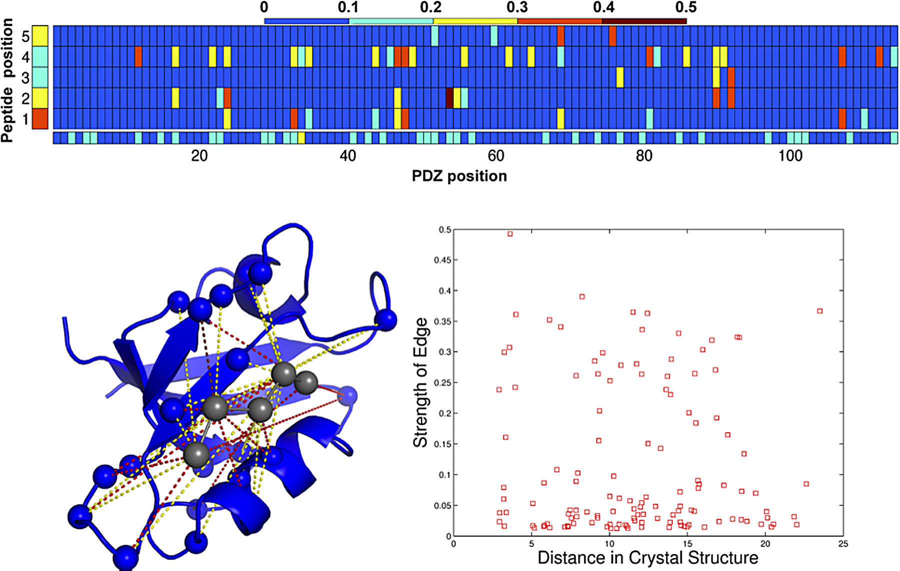
Model analysis. (Top) Average strength of the vector 2-norms for the PDZ positions (i.e., V_i), peptide positions (i.e., V_j), and potentially interacting pairs (i.e., W_i,j) in the model trained at λ_1,2=25. (Bottom left) Strong interactions highlighted in top panel, displayed on the NMR structure of the alpha syntropin PDZ (pdb id: 2PDZ). Color scheme same as above. (Bottom right) Average edge strength across 10 training splits plotted against distance in the 3D structure.

Despite the fact that no 3D structure information was used in learning the model, our method identifies several contacting residues as important for determining interaction specificity. This suggests that our data-driven approach might be capturing physically important interactions. To test this hypothesis further, we determined the average weight assigned to each possible amino acid pair for the top three interacting residue pairs across the models for the 10 training folds at λ_1,2=25. Figure 5 shows these weights with strong negative energies (i.e., favoring binding) in shades of blue and strong positive energies in shades of red. Darker shades correspond to stronger effects in both cases. The strongest interacting residue pair (PDZ position 54:peptide position 2) strongly favors interactions between oppositely charged arginine/lysine in the PDZ and glutamate in the peptide, while strongly penalizing aspartate/glutamate:glutamate between pairs of negatively charged residues, suggesting a strong electrostatic effect between these positions. Similar effects are seen in the other two interactions with glutamate:lysine favored between 48:1 and aspartate:threonine penalized between 12:4. Our method can thus provide structural information as well as insights into the biochemical determinants of binding affinity.

FIG. 5.

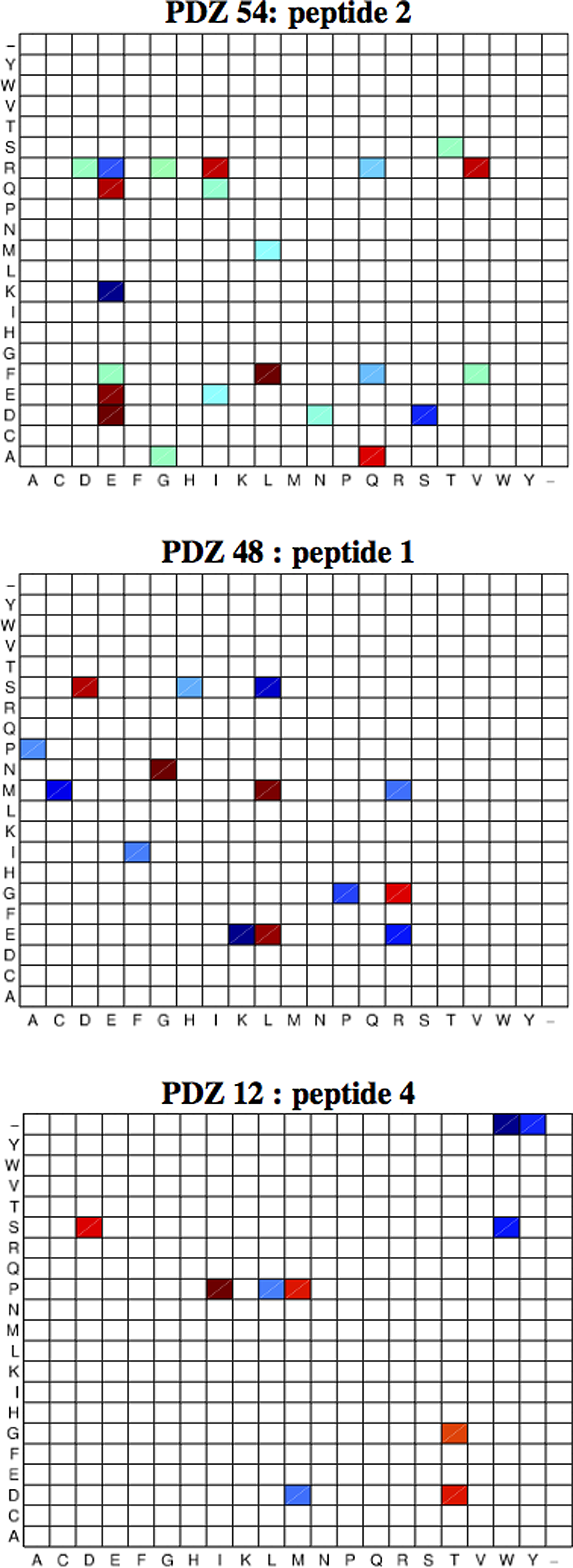
Average weights for amino acid pairs for the top three interacting residue pairs.

In summary, our results suggest that a large fraction of the binding affinity is due to interactions between a relatively small set of positions, not all spatially adjacent to the binding pocket. A larger set of weak interactions might have an additional small effect on binding; these might effect particular subfamilies of PDZs or might reflect allosteric affects related to alternate conformational states of the protein previously described in this family by Lockless and Ranganathan (1999).

3.3. From sequence determinants to sequence design

The accuracy and simplicity of our model allows us to rapidly evaluate the binding affinity of any PDZ–peptide pair. We demonstrate the utility of this approach by “designing” optimal binders for a given PDZ sequence. Using a model learned from the entire training set with λ_1,2 = 25, we searched all 5 residue peptides and determined the top 10 peptides by their predicted ΔG for each PDZ sequence. Figure 6 (left) shows the density of predicted binding energies of these PDZ:peptide pairs in blue and that of natural PDZ–peptide pairs binding energies in our training dataset in red. The predicted binding affinities of designed sequences are considerably lower than those of the natural sequences.

FIG. 6.

(Left) Density of predicted PDZ–peptide ΔG for designed peptides (blue) and experimental ΔG for natural PDZ–peptide pairs (red). (Right) Sequence logos for the top 10 peptide designs for SHANK1, CHAPSYN, and PSD95 (top, middle, and bottom).

While the designed sequences include the natural substrates (at close to their predicted affinities, as discussed above), they also include a diverse array of alternatives. Figure 6 (right) shows sequence logos of the top 10 designed peptides for 3 different PDZs. Even among these sets of top predicted binders, we see interesting diversity among the peptides, suggesting novel designs potentially worthy of experimental evaluation.

4. Discussion and Conclusion

We have developed a graphical model that is highly predictive of the ΔG of binding in protein:protein interactions, while providing an interpretable and designable basis for its predictions. The notion of modularity is fundamental to the idea of a graphical model. Hence these models form a powerful and natural tool to solve problems involving complex probability distributions over many random variables, like the ones here. Due to the natural equivalence between the graph structure of a model and the structure of spatial interactions in proteins, graphical models have seen considerable use in modeling various aspects of proteins: in recognizing structural motifs (Liu et al., 2009; Menke et al., 2010; Moitra et al., 2012), in protein structure alignments (Xu et al., 2006), and in modeling dynamics (Razavian et al., 2012). A growing body of work using graphical models to capture correlated mutations in protein families has also seen substantial success in predicting residue–residue contacts in the protein structure (Marks et al., 2011; Morcos et al., 2011; Nugent and Jones, 2012; Jones et al., 2012; Kamisetty et al., 2013), highlighting the power of these models.

While basing the modeling of ΔG on sequence and data is fundamentally different from structure-based predictors, which employ physics-based models and analysis of side-chain (and potentially backbone) conformations to assess interactions [e.g., Guerois et al. (2002); Kortemme and Baker (2002); Smith and Kortemme (2010)], we note that structure-based undirected graphical models have been used to predict ΔG (Kamisetty et al., 2008, 2011a). The integration of the structure-based approach and the sequence + data-based approach provides an interesting future direction. Our preliminary work on such integration for individual proteins (Kamisetty et al., 2009) provides evidence that the two viewpoints can be complementary and enable better prediction than either alone.

The method we developed here could be applied to any pair of interacting protein families with a similar extent of quantitative binding data. Due to their size and easy availability, PDZ domains form a “model system” for studying protein–protein interactions (Sheng and Sala, 2001; Kurakin et al., 2007; Tonikian et al., 2008; Chen et al., 2008). They are involved in formation of protein complexes that are involved in cellular signal transduction and neural circuitry (Sheng and Sala, 2001) and so make an interesting test case from the point of view of protein engineering (Fuh et al., 2000) and drug design (Saro et al., 2007).

We demonstrated that our models can be used to design novel peptides that interact strongly with a given PDZ domain. This approach could be extended using sampling or other inferential techniques to design a desired interaction, rather than only the peptide, and to scale up to larger sets of involved residues.

Footnotes

Acknowledgments

This work is supported in part by U.S. NSF grant IIS-0905193 (C.J.L. and C.B.K.) and U.S. NIH P41 GM103712 (C.J.L.).

Author Disclosure Statement

The authors declare that no competing financial interests exist.

References

Balakrishnan

, Kamisetty

, Carbonell

, et al. 2011. Learning generative models for protein fold families. Proteins Struct. Funct. Bioinform. 79, 1061–1078.

Bordner

, and Mittelmann

2010. MultiRTA: a simple yet accurate method for predicting peptide binding affinities for multiple class II MHC allotypes. BMC Bioinform., 11, 482.

Brannetti

, Via

, Cestra

, et al. 2000. SH3-SPOT: an algorithm to predict preferred ligands to different members of the SH3 gene family. J. Mol. Biol., 298, 313–328.

Chen

, Chang

, Allen

, et al. 2008. Predicting PDZ domain-peptide interactions from primary sequences. Nat. Biotechnol., 26, 1041–1045.

Fields

, and Song

1989. A novel genetic system to detect protein-protein interactions. Nature, 340, 245–246.

Fong

, Keating

, and Singh

2004. Predicting specificity in bZIP coiled-coil protein interactions. Genome Biol., 5, R11.

Fuh

, Pisabarro

, Li

, et al. 2000. Analysis of PDZ domain-ligand interactions using carboxyl-terminal phage display. J. Biol. Chem., 275, 21486–21491.

Grigoryan

, Reinke

, and Keating

2009. Design of protein-interaction specificity gives selective bZIP-binding peptides. Nature, 458, 859–864.

Guerois

, Nielsen

J.E.

, and Serrano

2002. Predicting changes in the stability of proteins and protein complexes: a study of more than 1000 mutations. J. Mol. Biol., 320, 369–387.

10.

Jones

D.T.

, Buchan

D.W.

, Cozzetto

, and Pontil

2012. Psicov: precise structural contact prediction using sparse inverse covariance estimation on large multiple sequence alignments. Bioinformatics, 28, 184–190.

11.

Kamisetty

, Ghosh

, Bailey-Kellogg

, and Langmead

2009. Modeling and Inference of sequence-structure specificity. In Proceedings of the 8th International Conference on Computational Systems Bioinformatics (CSB), pp. 91–101.

12.

Kamisetty

, Ovchinnikov

, and Baker

2013. Assessing the utility of coevolution-based residue–residue contact predictions in a sequence-and structure-rich era. Proc. Natl. Acad. Sci. USA, 110, 15674–15679.

13.

Kamisetty

, Ramanathan

, Bailey-Kellogg

, and Langmead

2011a. Accounting for conformational entropy in predicting binding free energies of protein-protein interactions. Proteins, 79, 444–462.

14.

Kamisetty

, Xing

, and Langmead

2008. Free energy estimates of all-atom protein structures using generalized belief propagation. J. Comput. Biol., 15, 755–766.

15.

Kamisetty

, Xing

, and Langmead

2011b. Approximating correlated equilibria using relaxations on the marginal polytope. In Proceedings of the 28th International Conference on Machine Learning (ICML), pp. 1153–1160.

16.

Kortemme

, and Baker

2002. A simple physical model for binding energy hot spots in protein-protein complexes. Proc. Natl. Acad. Sci. USA, 99, 14116–14121.

17.

Kurakin

, Swistowski

, Wu

, and Bredesen

2007. The pdz domain as a complex adaptive system. PLoS ONE, 2, e953.

18.

, Yi

Z.-P.

, Laskowski

, et al. 2005. Analysis of sequence-reactivity space for protein-protein interactions. Proteins Struct. Funct. Bioinform. 58, 661–671.

19.

Liu

, Carbonell

, Gopalakrishnan

, and Weigele

2009. Conditional graphical models for protein structural motif recognition. J. Comput. Biol., 16, 639–657.

20.

Lockless

S.W.

, and Ranganathan

1999. Evolutionarily conserved pathways of energetic connectivity in protein families. Science, 286, 295–299.

21.

, Lu

, Qasim

, et al. 2001. Predicting the reactivity of proteins from their sequence alone: Kazal family of protein inhibitors of serine proteinases. Proc. Natl. Acad. Sci. USA, 98, 1410–1415.

22.

Marks

D.S.

, Colwell

L.J.

, Sheridan

, et al. 2011. Protein 3d structure computed from evolutionary sequence variation. PLoS ONE, 6, e28766.

23.

Meinshausen

, and Bühlmann

2006. High-dimensional graphs and variable selection with the lasso. Ann. Stat., 34, 1436–1462.

24.

Menke

, Berger

, and Cowen

2010. Markov random fields reveal an n-terminal double beta-propeller motif as part of a bacterial hybrid two-component sensor system. PNAS, 107, 4069–4074.

25.

Moitra

, Tirupula

, Klein-Seetharaman

, and Langmead

2012. A minimal ligand binding pocket within a network of correlated mutations identified by multiple sequence and structural analysis of G protein coupled receptors. BMC Biophys., 5, 13.

26.

Morcos

, Pagnani

, Lunt

, et al. 2011. Direct-coupling analysis of residue coevolution captures native contacts across many protein families. Proc. Natl. Acad. Sci. USA, 108, E1293–E1301.

27.

Nielsen

, Lundegaard

, Blicher

, et al. 2007. NetMHCpan, a method for quantitative predictions of peptide binding to any HLA-A and -B locus protein of known sequence. PLoS ONE, 2, e796.

28.

Nugent

, and Jones

D.T.

2012. Accurate de novo structure prediction of large transmembrane protein domains using fragment-assembly and correlated mutation analysis. Proc. Natl. Acad. Sci. USA, 109, E1540–E1547.

29.

Peters

, Sidney

, Bourne

, et al. 2005. The immune epitope database and analysis resource: from vision to blueprint. PLoS Biol., 3, e91.

30.

Razavian

, Kamisetty

, and Langmead

2012. Learning generative models of molecular dynamics. BMC Genomics, 13, S5.

31.

Saro

, Li

, Rupasinghe

, et al. 2007. A thermodynamic ligand binding study of the third pdz domain (pdz3) from the mammalian neuronal protein psd-95. Biochemistry, 46, 6340–6352.

32.

Schmidt

, van der Berg

, Friedlander

M.P.

, and Murphy

2009. Optimizing costly functions with simple constraints:a limited-memory projected quasi-newton algorithm. AISTATS, 5, 456–463.

33.

Shao

, Tan

, Voss

, et al. 2010. A regression framework incorporating quantitative and negative interaction data improves quantitative prediction of PDZ domain-peptide interaction from primary sequence. Bioinformatics, 27, 383–390.

34.

Sheng

, and Sala

2001. Pdz domains and the organization of supramolecular complexes. Annu. Rev. Neurosci., 24, 1–29.

35.

Smith

, and Kortemme

2010. Structure-based prediction of the peptide sequence space recognized by natural and synthetic pdz domains. J. Mol. Biol. 402, 460–474.

36.

Stiffler

, Chen

, Grantcharova

, et al. 2007. Pdz domain binding selectivity is optimized across the mouse proteome. Science, 317, 364–369.

37.

Thomas

, Ramakrishnan

, and Bailey-Kellogg

2008. Graphical models of residue coupling in protein families. IEEE/ACM Trans. Comput. Biol. Bioinform., 5, 183–197.

38.

Thomas

, Ramakrishnan

, and Bailey-Kellogg

2009a. Graphical models of protein-protein interaction specificity from correlated mutations and interaction data. Proteins Struct. Funct. Bioinform. 76, 911–929.

39.

Thomas

, Ramakrishnan

, and Bailey-Kellogg

2009b. Protein design by sampling an undirected graphical model of residue constraints. IEEE/ACM Trans. Comput. Biol. Bioinform. 6, 506–516.

40.

Tonikian

, Zhang

, Sazinsky

, et al. 2008. A specificity map for the PDZ domain family. PLoS Biol., 6, e239.

41.

Wang

, Sidney

, Dow

, et al. 2008. A systematic assessment of MHC class II peptide binding predictions and evaluation of a consensus approach. PLoS Comp. Biol., 4, e1000048.

42.

, Jiao

, and Berger

2006. A parameterized algorithm for protein structure alignment. In Proceedings of International Symposium on Research in Computational Molecular Biology, Springer Lecture Notes in Computer Science 3903/2006, pp. 488–499.

43.

Zhang

, Udaka

, Mamitsuka

, and Zhu

2012. Toward more accurate pan-specific MHC-peptide binding prediction: a review of current methods and tools. Brief. Bioinform., 13, 350–364.