Medical Reasoning with Rough-Set Influence Diagrams

1. Introduction

There are several important capabilities of a medical reasoning system: diagnosis, prediction, treatment planning, etc. (Kao, 2008; Kao and Li, 2005; Kononenko, 2001; Leibovici et al., 2000; Li and Kao, 2005; Long, 2001). Diagnosis is the process of reconstructing past facts from observed evidence. Prediction is the process of projecting the evidence from hypotheses. Treatment planning is reasoning about the costs and effectiveness of treatments on patients. Usually, medical practice requires various kinds of reasoning to be carried out simultaneously. Hence, the capability for multiple reasoning tasks is critical to the performance of medical decision support systems. Moreover, medical expert systems become more complex when considering the mechanisms of the human body and their mutual interactions with environmental factors.

In the field of medical informatics, the graphical decision models such as Bayesian networks and influence diagrams have been widely used (Jensen, 2001; Kao, 2008; Kao and Li, 2005; Li and Kao, 2005; López-Díaz and Rodríguez-Muñiz, 2007; Neapolian, 2004; Nease and Owens, 1997; Oliver and Smith, 1990; Owens et al., 1997; Pearl, 1997). Influence diagrams are originally proposed as a compact representation of decision trees for symmetric decision scenarios, and are now regarded more as an extension of Bayesian networks (Pearl, 1997). Influence diagrams are a graphical technique for a decision problem under uncertainty (Howard and Matheson, 1981; Nease and Owens, 1997; Tatman and Shachter, 1990), and useful as knowledge representation and decision models (Jensen, 2001; Nease and Owens, 1997; Oliver and Smith, 1990; Shachter, 1986; Tatman and Shachter, 1990). Various methods have been developed for evaluating influence diagrams. In previous studies, the main numerical models of the influence diagrams used to be probability distributions (Howard and Matheson, 1981; Shachter, 1986).

There are several advantages in evaluating a problem using influence diagram operations. The analyst can use the representation that is natural to the decision maker and the algorithm executes the inference and analysis intelligently. The influence diagram solution procedure can also result in significant gains in efficiency. Conditional independence is clearly exhibited in the diagram, so the size of intermediate calculations can be reduced, resulting in considerable reductions in both processing time and memory requirements.

However, when imprecise knowledge from data sets is involved in the systems, how to reason from approximate information becomes a main issue in evaluating influence diagrams effectively. This study proposes an alternative numerical model for the knowledge in influence diagrams with rough sets. Rough set theory was first introduced by Pawlak (1982) as a tool for dealing with risk and impreciseness in decision making. The probabilistic approaches have been previously applied to rough set theory (Pawlak, 2002, 2003; Pawlak et al., 1988; Yao, 2003). Based on an approach recently proposed by Kao (2008), this study intends to propose an alternative numerical model for influence diagrams, which extends influence diagrams into rough-set influence diagrams. In rough-set influence diagrams, each chance node and value node is associated with the dependency, which expresses the uncertain features of the node. This study also develops rough-set-based influence diagrams that combine rough-set decision rules with the graphical structure of the influence diagrams found in medical settings.

The rest of this study is organized as follows. Section 2 illustrates the notations and the framework of influence diagrams. Section 3 describes the concept of rough sets and decision rules. Section 4 introduces how rough-set theory establishes the numerical model and decision support in influence diagrams. Section 5 illustrates the case studies of metastatic cancer and urinary tract infection. Section 6 gives the discussions and concluding remarks.

2. Influence Diagrams

Influence diagrams were originally introduced by Howard and Matheson (1981) as a compact representation of decision models. They are also thought of as an extension of Bayesian networks (Jensen, 2001; Pearl, 1997). An influence diagram is a directed acyclic graph (DAG) with three types of nodes: decision, chance, and value. A decision node, drawn as a rectangle, represents choices available to the decision makers. A chance node, drawn as a circle, represents random variables or uncertain quantities. A value node or utility node, shown as a diamond, represents the utility or the objective to be maximized in terms of expectation.

An influence diagram (ID) can be defined as \documentclass{aastex}\usepackage{amsbsy}\usepackage{amsfonts}\usepackage{amssymb}\usepackage{bm}\usepackage{mathrsfs}\usepackage{pifont}\usepackage{stmaryrd}\usepackage{textcomp}\usepackage{portland, xspace}\usepackage{amsmath, amsxtra}\pagestyle{empty}\DeclareMathSizes{10}{9}{7}{6}\begin{document} \begin{align*}{ \rm ID} = ( V , L , P ) \tag{1}\end{align*} \end{document}

where V denotes the set of nodes, L denotes the set of directed arcs, and P represents the numerical model. The composition of the node set V can be expressed as (2) \documentclass{aastex}\usepackage{amsbsy}\usepackage{amsfonts}\usepackage{amssymb}\usepackage{bm}\usepackage{mathrsfs}\usepackage{pifont}\usepackage{stmaryrd}\usepackage{textcomp}\usepackage{portland, xspace}\usepackage{amsmath, amsxtra}\pagestyle{empty}\DeclareMathSizes{10}{9}{7}{6}\begin{document} \begin{align*}V = V_{D} \cup V_{R} \cup V_{U} \tag{2}\end{align*} \end{document}

where V_D denotes the decision node sets, V_R represents the sets of chance nodes, and V_U denotes the value nodes to be optimized. This study uses the uppercase letters to represent the nodes and lowercase letters for the value of a variable.

There are two types of directed arcs: conditional arcs (into chance and value nodes) and informational arcs (into decision nodes). The meanings of the directed arcs depend on their destinations. Arcs pointing to value nodes represent approximate or functional dependence. Arcs into decision nodes imply time precedence and are informational; that is, they show which variables will be known to the decision makers before the decision is made. Conventionally, the knowledge of chance nodes is expressed with probability distributions while the outcomes of the value node are projected with a value table.

An influence diagram satisfies the following conditions:

(i) The directed graph has no cycles.

An example of influence diagrams for metastatic cancer and treatment is modified from Cooper (1984) as shown in Figure 1, where V = V_D ∪ V_R ∪ V_U, V_D = {T}, V_R = {B, C, I, M}, and V_U = {Q}.

OPEN IN VIEWER

FIG. 1.

An example of influence diagrams for metastatic cancer and treatment.

Metastatic cancer is a possible cause of a brain tumor and is also an explanation for increased total serum calcium. In Figure 1, there is one decision node T (treatment), which has two alternatives to take: yes or no. Four chance variables are relevant to the biological test and treatment problems: B (brain tumor), C (coma), I (increased total serum calcium), and M (metastatic cancer). The utility function Q (quality-adjusted life expectancy) is to be maximized. The meaning and states of the nodes are summarized in Table 1.

In Figure 1, the states of I and B determine the state of C. The states of I and B are conditioned on the manifestation of M. The outcome of M and the decision on T will determine the value of Q, where M provides the information prior to decision making. Usually, the causal relationships and decision rules in influence diagrams are expressed with probability distributions and a value table.

In medical informatics, influence diagrams are widely used knowledge representation and decision models under uncertainty. However, there are some limitations of utilizing the above approaches for solving medical reasoning problems:

(i) All associated probabilities are assumed to be non-fuzzy.

Hence, this study proposes an alternative approach for modeling the causal relationships in influence diagrams with rough sets.

3. Rough Sets

4. ROUGH-SET INFLUENCE DIAGRAMS (RSID)

Most studies on influence diagrams (Howard and Matheson, 1981; Nease and Owens, 1997; Pearl, 1997; Shachter, 1986) used to describe the dependency and its associated numerical model with probability distributions. However, when impreciseness is involved in the domain, the decision makers may need more flexible uncertainty measures for analysis. Rough set theory can be an alternative measure when faced with such a problem.

Given the influence diagrams structure and the original data sets, rough set theory provides a basis for extracting the knowledge and expressing the dependency among nodes in the influence diagrams. To represent the ontology, we define that a rough-set influence diagram is a directed acyclic graph RSID = (U, A, f ), where:

(i) U is the universe, a nonempty finite set of objects.

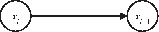
With every branch of (x_i, x_i+1) there is a directed arc from node x_i to x_i+1 as shown in Figure 2. The certainty, coverage, and strength of a branch (x_i, x_i+1) are defined as cer(x_i, x_i+1), cov(x_i, x_i+1), and σ(x_i, x_i+1), respectively.

OPEN IN VIEWER

FIG. 2.

A directed arc from node x_i to x_i+1.

A directed path from x₁ to x_n for x₁, x_n ∈ A denoted [x₁, x_n], is a sequence of nodes \documentclass{aastex}\usepackage{amsbsy}\usepackage{amsfonts}\usepackage{amssymb}\usepackage{bm}\usepackage{mathrsfs}\usepackage{pifont}\usepackage{stmaryrd}\usepackage{textcomp}\usepackage{portland, xspace}\usepackage{amsmath, amsxtra}\pagestyle{empty}\DeclareMathSizes{10}{9}{7}{6}\begin{document} $$x_{1} , x_{2} , \ldots , x_{i} , \ldots , x_{n} , 1 \leq i \leq n$$ \end{document} , as shown in Figure 3.

OPEN IN VIEWER

FIG. 3.

A directed path [x₁, x_n] from node x₁ to x_n.

Then, the certainty of a directed path [x₁, x_n] is defined as \documentclass{aastex}\usepackage{amsbsy}\usepackage{amsfonts}\usepackage{amssymb}\usepackage{bm}\usepackage{mathrsfs}\usepackage{pifont}\usepackage{stmaryrd}\usepackage{textcomp}\usepackage{portland, xspace}\usepackage{amsmath, amsxtra}\pagestyle{empty}\DeclareMathSizes{10}{9}{7}{6}\begin{document} \begin{align*}cer [ x_{1} , x_{n} ] = \mathop \prod \limits_{i = 1}^{n - 1} cer ( x_{1} , x_{n} ) \tag{18}\end{align*} \end{document}

The coverage of a directed path [x₁, x_n] is defined as \documentclass{aastex}\usepackage{amsbsy}\usepackage{amsfonts}\usepackage{amssymb}\usepackage{bm}\usepackage{mathrsfs}\usepackage{pifont}\usepackage{stmaryrd}\usepackage{textcomp}\usepackage{portland, xspace}\usepackage{amsmath, amsxtra}\pagestyle{empty}\DeclareMathSizes{10}{9}{7}{6}\begin{document} \begin{align*}cov [ x_{1} , x_{n} ] = \mathop \prod \limits_{i = 1}^{n - 1} cov ( x_{1} , x_{n} ) \tag{19}\end{align*} \end{document}

The strength of a directed path [x₁, x_n] is defined as \documentclass{aastex}\usepackage{amsbsy}\usepackage{amsfonts}\usepackage{amssymb}\usepackage{bm}\usepackage{mathrsfs}\usepackage{pifont}\usepackage{stmaryrd}\usepackage{textcomp}\usepackage{portland, xspace}\usepackage{amsmath, amsxtra}\pagestyle{empty}\DeclareMathSizes{10}{9}{7}{6}\begin{document} \begin{align*}\sigma [ x_{1} , x_{n} ] = \begin{cases} \sigma ( x_1 ) cer [ x_1 , x_n ] = \sigma ( x_{1} ) \mathop \prod \limits_{i = 1}^{n - 1} cer ( x_{1} , x_{n} ) \\ \sigma ( x_{n} ) cov [ x_{1} , x_{n} ] = \sigma ( x_{n} ) \mathop \prod \limits_{i = 1}^{n - 1} cov ( x_{1} , x_{n} ) \end{cases} \tag{20}\end{align*} \end{document}

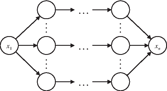
The set of all directed paths from x₁ to x_n denoted 〈x₁, x_n〉 as shown in Figure 4, where [x₁, x_n] ∈ 〈x₁, x_n〉.

OPEN IN VIEWER

FIG. 4.

The set, \documentclass{aastex}\usepackage{amsbsy}\usepackage{amsfonts}\usepackage{amssymb}\usepackage{bm}\usepackage{mathrsfs}\usepackage{pifont}\usepackage{stmaryrd}\usepackage{textcomp}\usepackage{portland, xspace}\usepackage{amsmath, amsxtra}\pagestyle{empty}\DeclareMathSizes{10}{9}{7}{6}\begin{document} $$\langle x_{1} , x_{n} \rangle$$ \end{document} , of all directed paths from node x₁ to x_n.

Then, the certainty of 〈x₁, x_n〉 is \documentclass{aastex}\usepackage{amsbsy}\usepackage{amsfonts}\usepackage{amssymb}\usepackage{bm}\usepackage{mathrsfs}\usepackage{pifont}\usepackage{stmaryrd}\usepackage{textcomp}\usepackage{portland, xspace}\usepackage{amsmath, amsxtra}\pagestyle{empty}\DeclareMathSizes{10}{9}{7}{6}\begin{document} \begin{align*}cer \langle x_{1} , x_{n} \rangle = \sum_{ [ x_{1} , x_{n} ] \in \langle x_{1} , x_{n} \rangle} cer [ x_{1} , x_{n} ] \tag{21}\end{align*} \end{document}

The coverage of 〈x₁, x_n〉 is \documentclass{aastex}\usepackage{amsbsy}\usepackage{amsfonts}\usepackage{amssymb}\usepackage{bm}\usepackage{mathrsfs}\usepackage{pifont}\usepackage{stmaryrd}\usepackage{textcomp}\usepackage{portland, xspace}\usepackage{amsmath, amsxtra}\pagestyle{empty}\DeclareMathSizes{10}{9}{7}{6}\begin{document} \begin{align*}cov \langle x_{1} , x_{n} \rangle = \sum_{ [ x_{1} , x_{n} ] \in \langle x_{1} , x_{n} \rangle} cov [ x_{1} , x_{n} ] \tag{22}\end{align*} \end{document}

The strength of 〈x₁, x_n〉 is \documentclass{aastex}\usepackage{amsbsy}\usepackage{amsfonts}\usepackage{amssymb}\usepackage{bm}\usepackage{mathrsfs}\usepackage{pifont}\usepackage{stmaryrd}\usepackage{textcomp}\usepackage{portland, xspace}\usepackage{amsmath, amsxtra}\pagestyle{empty}\DeclareMathSizes{10}{9}{7}{6}\begin{document} \begin{align*}\sigma \langle x_{1} , x_{n} \rangle = \sum \limits_{ [ x_{1} , x_{n} ] \in \langle x_{1} , x_{n} \rangle} \sigma [ x_{1} , x_{n} ] = \begin{cases} \sum \limits_{ [ x_{1} , x_{n} ] \in \langle x_{1} , x_{n} \rangle} \sigma ( x_{1} ) \mathop \prod \limits_{i = 1}^{n - 1} cer ( x_{1} , x_{n} ) \\ \sum \limits_{ [ x_{1} , x_{n} ] \in \langle x_{1} , x_{n} \rangle} \sigma ( x_{n} ) \mathop \prod \limits_{i = 1}^{n - 1} cov ( x_{1} , x_{n} ) \end{cases} \tag{23}\end{align*} \end{document}

The main objective of an influence diagram with a value node is to maximize the expected value (Shachter, 1986; Tatman and Shachter, 1990). To perform this, the following transformations are introduced. Consider the following cases:

Case 1: Removal of a chance node by summing it out of the joint can be accomplished, as shown in Figure 5. This corresponds to \documentclass{aastex}\usepackage{amsbsy}\usepackage{amsfonts}\usepackage{amssymb}\usepackage{bm}\usepackage{mathrsfs}\usepackage{pifont}\usepackage{stmaryrd}\usepackage{textcomp}\usepackage{portland, xspace}\usepackage{amsmath, amsxtra}\pagestyle{empty}\DeclareMathSizes{10}{9}{7}{6}\begin{document} \begin{align*} \begin{split} \sigma ( x_{5} \mid x_{1} , x_{2} , x_{3} ) \leftarrow \sum_{x_{4}} \sigma ( x_{4} , x_{5} \mid x_{1} , x_{2} , x_{3} ) \\ = \sum_{x_{4}} \sigma ( x_{5} \mid x_{2} , x_{3} , x_{4} ) \sigma ( x_{4} \mid x_{1} , x_{2} ) \end{split} \tag{24}\end{align*} \end{document}

OPEN IN VIEWER

FIG. 5.

Removal of a chance node x₄ into x₅ by summation.

Case 2: Arc reversal between two chance nodes, as shown in Figure 6, corresponds to the Bayes theorem and can be performed by the two-step operation as (25) and (26). \documentclass{aastex}\usepackage{amsbsy}\usepackage{amsfonts}\usepackage{amssymb}\usepackage{bm}\usepackage{mathrsfs}\usepackage{pifont}\usepackage{stmaryrd}\usepackage{textcomp}\usepackage{portland, xspace}\usepackage{amsmath, amsxtra}\pagestyle{empty}\DeclareMathSizes{10}{9}{7}{6}\begin{document} \begin{align*} \begin{split} \sigma ( x_{5} \mid x_{1} , x_{2} , x_{3} ) \leftarrow \sum_{x_{4}} \sigma ( x_{4} , x_{5} \mid x_{1} , x_{2} , x_{3} ) \\ = \sum_{x_{4}} \sigma ( x_{5} \mid x_{2} , x_{3} , x_{4} ) \sigma ( x_{4} \mid x_{1} , x_{2} ) \end{split} \tag{25}\end{align*} \end{document} \documentclass{aastex}\usepackage{amsbsy}\usepackage{amsfonts}\usepackage{amssymb}\usepackage{bm}\usepackage{mathrsfs}\usepackage{pifont}\usepackage{stmaryrd}\usepackage{textcomp}\usepackage{portland, xspace}\usepackage{amsmath, amsxtra}\pagestyle{empty}\DeclareMathSizes{10}{9}{7}{6}\begin{document} \begin{align*} \begin{split} \sigma ( x_ { 4 } \mid x_ { 1 } , x_ { 2 } , x_ { 3 } , x_ { 5 } ) \leftarrow \frac { \sigma ( x_ { 4 } , x_ { 5 } \mid x_ { 1 } , x_ { 2 } , x_ { 3 } ) } { \sigma ( x_ { 5 } \mid x_ { 1 } , x_ { 2 } , x_ { 3 } ) } \\ = \frac { \sigma ( x_ { 5 } \mid x_ { 2 } , x_ { 3 } , x_ { 4 } ) \sigma ( x_ { 4 } \mid x_ { 1 } , x_ { 2 } ) } { \sigma ( x_ { 5 } \mid x_ { 1 } , x_ { 2 } , x_ { 3 } ) } \end{split} \tag { 26 }\end{align*} \end{document}

OPEN IN VIEWER

FIG. 6.

Reversal of an arc from node x₄ to x₅.

Case 3: Removal of a chance node by expectation, as shown in Figure 7, can be accomplished as \documentclass{aastex}\usepackage{amsbsy}\usepackage{amsfonts}\usepackage{amssymb}\usepackage{bm}\usepackage{mathrsfs}\usepackage{pifont}\usepackage{stmaryrd}\usepackage{textcomp}\usepackage{portland, xspace}\usepackage{amsmath, amsxtra}\pagestyle{empty}\DeclareMathSizes{10}{9}{7}{6}\begin{document} \begin{align*}E [ U ( u \mid x_{1} , x_{2} , x_{3} ) ] \leftarrow E [ U_{x_{4}} ( E [ U ( u \mid x_{2} , x_{3} , x_{4} ) ] \mid x_{1} , x_{2} ) ] \tag{27}\end{align*} \end{document}

OPEN IN VIEWER

FIG. 7.

Removal of a chance node x₄ into u by expectation.

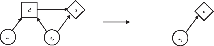
Case 4: Removal of a decision node by maximization, as shown in Figure 8, can be accomplished as \documentclass{aastex}\usepackage{amsbsy}\usepackage{amsfonts}\usepackage{amssymb}\usepackage{bm}\usepackage{mathrsfs}\usepackage{pifont}\usepackage{stmaryrd}\usepackage{textcomp}\usepackage{portland, xspace}\usepackage{amsmath, amsxtra}\pagestyle{empty}\DeclareMathSizes{10}{9}{7}{6}\begin{document} \begin{align*}E [ U ( u \mid x_{2} ) ] \leftarrow \max_{d} E [ U ( u \mid d , x_{2} ) ] \tag{28}\end{align*} \end{document}

OPEN IN VIEWER

FIG. 8.

Removal of a decision node d by maximization.

According to the cases above, the alternative numerical model based on rough set can be constructed for influence diagrams.

5. Numerical Examples

Example 1. Consider an influence diagram as shown in Figure. 1. According to (9), and (10), the certainty factors and value functions can be obtained in Table 2.

The objective of this problem is to maximize the expected utilities as follows. \documentclass{aastex}\usepackage{amsbsy}\usepackage{amsfonts}\usepackage{amssymb}\usepackage{bm}\usepackage{mathrsfs}\usepackage{pifont}\usepackage{stmaryrd}\usepackage{textcomp}\usepackage{portland, xspace}\usepackage{amsmath, amsxtra}\pagestyle{empty}\DeclareMathSizes{10}{9}{7}{6}\begin{document} \begin{align*}\max_{t} E [ U ( q \mid m , t ) ] = \max_{t} \sum q ( m , t ) \sigma ( m \mid b , c , i ) \tag{29}\end{align*} \end{document}

where σ(m|b, c, i) is the posterior (belief) function of m, and \documentclass{aastex}\usepackage{amsbsy}\usepackage{amsfonts}\usepackage{amssymb}\usepackage{bm}\usepackage{mathrsfs}\usepackage{pifont}\usepackage{stmaryrd}\usepackage{textcomp}\usepackage{portland, xspace}\usepackage{amsmath, amsxtra}\pagestyle{empty}\DeclareMathSizes{10}{9}{7}{6}\begin{document} \begin{align*} \begin{split} \sigma ( m \mid b , c , i ) = \frac { \sigma ( m , b , c , i ) } { \sigma ( b , c , i ) } \\ = \frac { \sigma ( m ) \sigma ( b \mid m ) \sigma ( i \mid m ) \sigma ( c \mid b , i ) } { \sum \limits_ { m } \sigma ( m ) \sigma ( b \mid m ) \sigma ( i \mid m ) \sigma ( c \mid b , i ) } \end{split} \tag { 30 } \end{align*} \end{document}

Suppose the observation c = 0 then: \documentclass{aastex}\usepackage{amsbsy}\usepackage{amsfonts}\usepackage{amssymb}\usepackage{bm}\usepackage{mathrsfs}\usepackage{pifont}\usepackage{stmaryrd}\usepackage{textcomp}\usepackage{portland, xspace}\usepackage{amsmath, amsxtra}\pagestyle{empty}\DeclareMathSizes{10}{9}{7}{6}\begin{document} \begin{align*}\sigma ( m = 1 \mid c = 0 ) = \frac { { \sum \limits_ { b , c = 0 , i } \sigma ( m = 1 ) \sigma ( b \mid m = 1 ) \sigma ( i \mid m = 1 ) \sigma ( c = 0 \mid b , i ) } } { \sum \limits_ { b , c = 0 , i , m } \sigma ( m ) \sigma ( b \mid m ) \sigma ( i \mid m ) \sigma ( c = 0 \mid b , i ) } \tag { 31 } \end{align*} \end{document}

The numerator and denominator of (31) can be computed as \documentclass{aastex}\usepackage{amsbsy}\usepackage{amsfonts}\usepackage{amssymb}\usepackage{bm}\usepackage{mathrsfs}\usepackage{pifont}\usepackage{stmaryrd}\usepackage{textcomp}\usepackage{portland, xspace}\usepackage{amsmath, amsxtra}\pagestyle{empty}\DeclareMathSizes{10}{9}{7}{6}\begin{document} \begin{align*} \sum_{b , c = 0 , i} \sigma ( m = 1 ) \sigma ( b \mid m = 1 ) \sigma ( i \mid m = 1 ) \sigma ( c = 0 \mid b , i ) \\ = \sigma ( m = 1 ) \sigma ( b = 1 \mid m = 1 ) \sigma ( i = 1 \mid m = 1 ) \sigma ( c = 0 \mid b = 1 , i = 1 ) + \\ \sigma ( m = 1 ) \sigma ( b = 1 \mid m = 1 ) \sigma ( i = 0 \mid m = 1 ) \sigma ( c = 0 \mid b = 1 , i = 0 ) + \\ \sigma ( m = 1 ) \sigma ( b = 0 \mid m = 1 ) \sigma ( i = 1 \mid m = 1 ) \sigma ( c = 0 \mid b = 0 , i = 1 ) + \\ \sigma ( m = 1 ) \sigma ( b = 0 \mid m = 1 ) \sigma ( i = 0 \mid m = 1 ) \sigma ( c = 0 \mid b = 0 , i = 0 ) \\ = 0.2 \times 0.7 \times 0.8 \times 0.1 + 0.2 \times 0.7 \times 0.2 \times 0.4 + \\ 0.2 \times 0.3 \times 0.8 \times 0.4 + 0.2 \times 0.3 \times 0.2 \times 0.95 \\ = 0.053\end{align*} \end{document} \documentclass{aastex}\usepackage{amsbsy}\usepackage{amsfonts}\usepackage{amssymb}\usepackage{bm}\usepackage{mathrsfs}\usepackage{pifont}\usepackage{stmaryrd}\usepackage{textcomp}\usepackage{portland, xspace}\usepackage{amsmath, amsxtra}\pagestyle{empty}\DeclareMathSizes{10}{9}{7}{6}\begin{document} \begin{align*} \sum_{b , c = 0 , i} \sigma ( m = 0 ) \sigma ( b \mid m = 0 ) \sigma ( i \mid m = 0 ) \sigma ( c = 0 \mid b , i ) \\ = \sigma ( m = 0 ) \sigma ( b = 1 \mid m = 0 ) \sigma ( i = 1 \mid m = 0 ) \sigma ( c = 0 \mid b = 1 , i = 1 ) + \\ \sigma ( m = 0 ) \sigma ( b = 1 \mid m = 0 ) \sigma ( i = 0 \mid m = 0 ) \sigma ( c = 0 \mid b = 1 , i = 0 ) + \\ \sigma ( m = 0 ) \sigma ( b = 0 \mid m = 0 ) \sigma ( i = 1 \mid m = 0 ) \sigma ( c = 0 \mid b = 0 , i = 1 ) + \\ \sigma ( m = 0 ) \sigma ( b = 0 \mid m = 0 ) \sigma ( i = 0 \mid m = 0 ) \sigma ( c = 0 \mid b = 0 , i = 0 ) \\ = 0.8 \times 0.2 \times 0.2 \times 0.1 + 0.8 \times 0.2 \times 0.8 \times 0.4 + \\ 0.8 \times 0.8 \times 0.2 \times 0.4 + 0.8 \times 0.8 \times 0.8 \times 0.95 \\ = 0.592\end{align*} \end{document}

Then (31) can be obtained as \documentclass{aastex}\usepackage{amsbsy}\usepackage{amsfonts}\usepackage{amssymb}\usepackage{bm}\usepackage{mathrsfs}\usepackage{pifont}\usepackage{stmaryrd}\usepackage{textcomp}\usepackage{portland, xspace}\usepackage{amsmath, amsxtra}\pagestyle{empty}\DeclareMathSizes{10}{9}{7}{6}\begin{document} \begin{align*} \sigma ( m = 1 \mid c = 0 ) = \frac { \sum_ { b , c = 0 , i } \sigma ( m = 1 ) \sigma ( b \mid m = 1 ) \sigma ( i \mid m = 1 ) \sigma ( c = 0 \mid b , i ) } { \sum_ { b , c = 0 , i , m } \sigma ( m ) \sigma ( b \mid m ) \sigma ( i \mid m ) \sigma ( c = 0 \mid b , i ) } \\ = \frac { 0.053 } { 0.053 + 0.592 } = 0.0822 \end{align*} \end{document} \documentclass{aastex}\usepackage{amsbsy}\usepackage{amsfonts}\usepackage{amssymb}\usepackage{bm}\usepackage{mathrsfs}\usepackage{pifont}\usepackage{stmaryrd}\usepackage{textcomp}\usepackage{portland, xspace}\usepackage{amsmath, amsxtra}\pagestyle{empty}\DeclareMathSizes{10}{9}{7}{6}\begin{document} \begin{align*} \sigma ( m = 0 \mid c = 0 ) = \frac { \sum_ { b , c = 0 , i } \sigma ( m = 0 ) \sigma ( b \mid m = 0 ) \sigma ( i \mid m = 0 ) \sigma ( c = 0 \mid b , i ) } { \sum_ { b , c = 0 , i , m } \sigma ( m ) \sigma ( b \mid m ) \sigma ( i \mid m ) \sigma ( c = 0 \mid b , i ) } \\ = \frac { 0.592 } { 0.053 + 0.592 } = 0.9178 \end{align*} \end{document}

Hence \documentclass{aastex}\usepackage{amsbsy}\usepackage{amsfonts}\usepackage{amssymb}\usepackage{bm}\usepackage{mathrsfs}\usepackage{pifont}\usepackage{stmaryrd}\usepackage{textcomp}\usepackage{portland, xspace}\usepackage{amsmath, amsxtra}\pagestyle{empty}\DeclareMathSizes{10}{9}{7}{6}\begin{document} \begin{align*} & E [ U ( q \mid m , t = { \rm Yes} ) ] \\ & = \sum_{b , i} q ( m = 1 , t = { \rm Yes} ) \sigma ( m = 1 \mid c = 0 ) + \sum_{b , i} q ( m = 0 , t = { \rm Yes} ) \sigma ( m = 0 \mid c = 0 ) \\ & = q ( m = 1 , t = { \rm Yes} ) \sum_{b , i} \sigma ( m = 1 \mid c = 0 ) + q ( m = 0 , t = { \rm Yes} ) \sum_{b , i} \sigma ( m = 0 \mid c = 0 ) \\ & = 70 \times 0.0822 + 80 \times 0.9178 \\ = 79.178\end{align*} \end{document} \documentclass{aastex}\usepackage{amsbsy}\usepackage{amsfonts}\usepackage{amssymb}\usepackage{bm}\usepackage{mathrsfs}\usepackage{pifont}\usepackage{stmaryrd}\usepackage{textcomp}\usepackage{portland, xspace}\usepackage{amsmath, amsxtra}\pagestyle{empty}\DeclareMathSizes{10}{9}{7}{6}\begin{document} \begin{align*} & E [ U ( q \mid m , t = { \rm No} ) ] \\ & = \sum_{b , i} q ( m = 1 , t = { \rm No} ) \sigma ( m = 1 \mid c = 0 ) + \sum_{b , i} q ( m = 0 , t = { \rm No} ) \sigma ( m = 0 \mid c = 0 ) \\ & = q ( m = 1 , t = { \rm No} ) \sum_{b , i} \sigma ( m = 1 \mid c = 0 ) + q ( m = 0 , t = { \rm No} ) \sum_{b , i} \sigma ( m = 0 \mid c = 0 ) \\ & = 20 \times 0.0822 + 100 \times 0.9178 \\ & = 93.424\end{align*} \end{document}

Hence, the optimal decision to maximize the utilities is \documentclass{aastex}\usepackage{amsbsy}\usepackage{amsfonts}\usepackage{amssymb}\usepackage{bm}\usepackage{mathrsfs}\usepackage{pifont}\usepackage{stmaryrd}\usepackage{textcomp}\usepackage{portland, xspace}\usepackage{amsmath, amsxtra}\pagestyle{empty}\DeclareMathSizes{10}{9}{7}{6}\begin{document} \begin{align*}\max_{t}E [ U ( q \mid m , t ) ] = \max_{t} \{ 79.178 , 93.424 \} = 93.424\end{align*} \end{document}

where the optimal decision is t = No (no treatment).

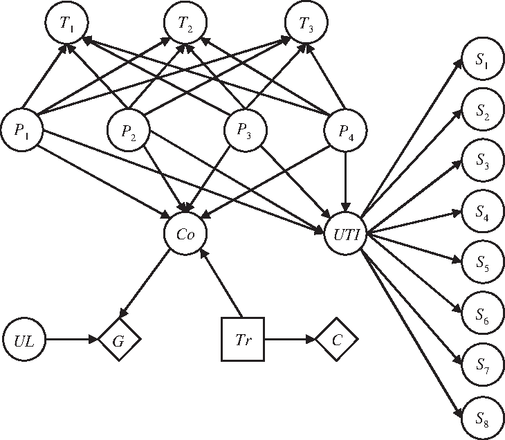
Example 2. Consider a case of urinary tract infection (UTI) modified from Leibovici et al. (2000), as shown in Figure 9.

OPEN IN VIEWER

FIG. 9.

A case of urinary tract infection (UTI).

There are one decision node V_D = {Tr}, two value nodes V_u = {C, G}, and eighteen chance nodes V _R  = {C_o, UL, UTI, P₁, P₂, P₃, P₄, T₁, T₂, T₃, S₁, S₂, S₃, S₄, S₅, S₆, S₇, S₈} relevant to the urinary tract infection and treatments. The descriptions and states of the nodes are listed as below.

The descriptions and states of the nodes are summarized in Table 3. Consider the evidence that a patient has suffered from frequent micturition (S₂ = 1), flank pain (S₃ = 1), urinary symptoms (S₄ = 1), and leucocyturie (S₇ = 1), but has not fallen into a suprapubic pain (S₁ = 0), serum albumin (S₅ = 0), fever (S₆ = 0), or hematuria (S₈ = 0). The evidence set is {S₁ = 0,S₂ = 1,S₃ = 1,S₄ = 1,S₅ = 0,S₆ = 0,S₇ = 1,S₈ = 0}. We intend to maximize the expected net gain of life expectancy according to the symptoms as below \documentclass{aastex}\usepackage{amsbsy}\usepackage{amsfonts}\usepackage{amssymb}\usepackage{bm}\usepackage{mathrsfs}\usepackage{pifont}\usepackage{stmaryrd}\usepackage{textcomp}\usepackage{portland, xspace}\usepackage{amsmath, amsxtra}\pagestyle{empty}\DeclareMathSizes{10}{9}{7}{6}\begin{document} \begin{align*}\max_{tr} Gain = E [ G ( co , ul ) - C ( tr ) ] \tag{32}\end{align*} \end{document}

Following the assumption (Kao and Li, 2005) that the underlying disorder and health status can be converted to an equivalent base year; in this case, 35 years base and 1 year gained in life can be regarded as equivalent to $55,000 (given ul) (Leibovici et al., 2000). The gain can be computed as below \documentclass{aastex}\usepackage{amsbsy}\usepackage{amsfonts}\usepackage{amssymb}\usepackage{bm}\usepackage{mathrsfs}\usepackage{pifont}\usepackage{stmaryrd}\usepackage{textcomp}\usepackage{portland, xspace}\usepackage{amsmath, amsxtra}\pagestyle{empty}\DeclareMathSizes{10}{9}{7}{6}\begin{document} \begin{align*} \begin{split} & Gain \\ & = 55 , 000 \times \sigma ( co \mid s_{1} , s_{2} , \ldots , s_{8} ) - C ( tr ) \\ & = 55 , 000 \times \sum_{ \scriptstyle p_{1} , p_{2} , p_{3} , p_{4} , \atop \scriptstyle tr , uti} \sigma ( co \mid p_{1} , p_{2} , p_{3} , p_{4} , tr , uti , s_{1} , s_{2} , \ldots , s_{8} ) - C ( tr ) \end{split} \tag{33}\end{align*} \end{document}

Selected rough sets of this case are shown in Table 4.

We adopt the stochastic simulation method as shown in Table 5 to obtain the optimal treatment and utility. The results are shown in Table 6. The optimal treatment is tr₃, which brings about $22,820 equivalent net gain.

6. Conclusions and Future Plans

This study proposes an alternative numerical framework for influence diagrams, rough sets, and develops the rough-set influence diagrams that combine decision rules with the graphical structure in medical settings. Considering the imprecise knowledge, this study formulates the causal relationships and the decision rules among the nodes (attributes) with rough sets from information systems. The proposed knowledge model provides a comprehensive schema for knowledge representation and decision support.

For future studies, there are several potential themes: (1) to integrate analysis with rough sets in various graphical decision models, including Bayesian networks, decision trees, and influence diagrams; (2) hybrid decision analysis with fuzzy sets and rough sets in graphical decision models; and (3) potential applications of intelligent decision support with rough sets, such as supply chain management, business strategic analysis, and biomedicine.