Sorting by Transpositions is an NP-hard problem for which several polynomial-time approximation algorithms have been developed. Hartman and Shamir (2006) developed a 1.5-approximation \documentclass{aastex}\usepackage{amsbsy}\usepackage{amsfonts}\usepackage{amssymb}\usepackage{bm}\usepackage{mathrsfs}\usepackage{pifont}\usepackage{stmaryrd}\usepackage{textcomp}\usepackage{portland, xspace}\usepackage{amsmath, amsxtra}\pagestyle{empty}\DeclareMathSizes{10}{9}{7}{6}\begin{document}
$$\bf { O ( n^ \frac { 3 } { 2 } \sqrt { \bold log \,\,n } ) } $$
\end{document} algorithm, whose running time was improved to O(nlogn) by Feng and Zhu (2007) with a data structure they defined, the permutation tree. Elias and Hartman (2006) developed a 1.375-approximation O(n2) algorithm, and Firoz et al. (2011) claimed an improvement to the running time, from O(n2) to O(nlogn), by using the permutation tree. We provide counter-examples to the correctness of Firoz et al.'s strategy, showing that it is not possible to reach a component by sufficient extensions using the method proposed by them. In addition, we propose a 1.375-approximation algorithm, modifying Elias and Hartman's approach with the use of permutation trees and achieving O(nlogn) time.
1 Introduction
In the study of genome rearrangements, chromosomes are commonly modeled by permutations (Fertin et al., 2009). In the Sorting by Transpositions (SBT) problem, the aim is to find the minimum number of contiguous block interchanges that transforms a given permutation of n elements into the identity permutation; this minimum is called the transposition distance (Bafna and Pevzner, 1998). SBT is an NP-hard problem (Bulteau et al., 2012), and tight bounds on the transposition distance are known (Bafna and Pevzner, 1998; Labarre, 2006), but exact values for the transposition distance are known only for a few classes of permutations (Cunha et al., 2013a; Labarre, 2006). Several approaches to handling the SBT problem have been considered. Our focus is to explore approximation algorithms for estimating the transposition distance between permutations, providing better practical results or lowering time complexities.
Bafna and Pevzner (1998) designed a 1.5-approximation O(n2) algorithm, where n is the length of the input permutation, based on the cycle structure of the breakpoint graph. Hartman and Shamir (2006) later proposed an easier 1.5-approximation algorithm that exploits a balanced tree data structure to decrease the running time to \documentclass{aastex}\usepackage{amsbsy}\usepackage{amsfonts}\usepackage{amssymb}\usepackage{bm}\usepackage{mathrsfs}\usepackage{pifont}\usepackage{stmaryrd}\usepackage{textcomp}\usepackage{portland, xspace}\usepackage{amsmath, amsxtra}\pagestyle{empty}\DeclareMathSizes{10}{9}{7}{6}\begin{document}
$$O ( n^ \frac { 3 } { 2 } \sqrt { \log n } )$$
\end{document}. Feng and Zhu (2007) developed another balanced tree data structure—the permutation tree—and further decreased the complexity of Hartman and Shamir's 1.5-approximation algorithm to O(nlogn). Elias and Hartman (2006) obtained, by a thorough computational case analysis of cycles of the breakpoint graph, a 1.375-approximation algorithm that runs in O(n2) time. Firoz et al. (2011) claimed that this 1.375-approximation algorithm could be easily adapted to run in O(nlogn) time if a permutation tree was used.
In the present article, we show that Firoz et al.'s usage of the so-called “Query” procedure to extend a full configuration into a component fails in some situations. We provide an infinite family of permutations for which Firoz et al.'s approach does not find an \documentclass{aastex}\usepackage{amsbsy}\usepackage{amsfonts}\usepackage{amssymb}\usepackage{bm}\usepackage{mathrsfs}\usepackage{pifont}\usepackage{stmaryrd}\usepackage{textcomp}\usepackage{portland, xspace}\usepackage{amsmath, amsxtra}\pagestyle{empty}\DeclareMathSizes{10}{9}{7}{6}\begin{document}
$$11/ 8$$
\end{document}-sequence, proving that the immediate use of a permutation tree is not enough to lower the running time of the 1.375-approximation algorithm to O(nlogn). We rectify the use of the permutation tree, proposing a new algorithm that generalizes the bad small component strategy of Elias and Hartman toward bad small full configurations, achieving both the 1.375 approximation ratio and the O(nlogn) time complexity. We thus achieve the best approximation ratio and time complexity for the SBT problem, known so far. The correctness of our algorithm is asserted via a branch-and-bound analysis that finds an 11/8-sequence for every combination of bad small full configurations.
The present article is organized as follows: section 2 contains basic definitions, some background on Elias and Hartman's algorithm and on the permutation tree data structure; section 3 discusses Firoz et al.'s approach on the use of a permutation tree to speed up the 1.375-approximation algorithm and provides counterexamples that establish the incorrectness of their approach; section 4 presents a strategy to determine the existence and to find a sequence of two transpositions, in which both are 2-moves, in linear time; section 5 describes our proposed 1.375-approximation O(nlogn) algorithm for SBT, proving its correctness and its worst-case running time; and section 6 contains our final remarks.
2 Background
For our purposes, a gene is represented by a unique integer and a chromosome with n genes is a permutation π = [π0π1π2 … πnπn+1], where π0 = 0, πn+1 = n + 1 and each πi, where 1 ≤ i ≤ n, is a unique integer in the range 1, … , n. The transposition t(i, j, k) applied to π, where 1 ≤ i < j < k ≤ n + 1, is the permutation π·t (i, j, k) in which the two contiguous blocks πiπi+1 … πj−1 and πjπj+1 … πk−1 are interchanged. A sequence of q transpositions t1, t2, … , tq sorts a permutation \documentclass{aastex}\usepackage{amsbsy}\usepackage{amsfonts}\usepackage{amssymb}\usepackage{bm}\usepackage{mathrsfs}\usepackage{pifont}\usepackage{stmaryrd}\usepackage{textcomp}\usepackage{portland, xspace}\usepackage{amsmath, amsxtra}\pagestyle{empty}\DeclareMathSizes{10}{9}{7}{6}\begin{document}
$$\pi \ { \rm if} \ \pi \cdot t_1 \cdot t_2 \ldots .\,.\, t_q = \iota$$
\end{document}, where ι is the identity permutation [0 1 2 … nn + 1]. The transposition distance of π, denoted d(π), is the length of a minimum sequence of transpositions that sorts π.
The breakpoint graph Nontrivial bounds on the transposition distance were obtained by using the breakpoint graph (Bafna and Pevzner, 1998). Given a permutation π, the breakpoint graph of π is G(π) = (V,R ∪ D). The set of vertices is V = {0, −1, + 1, −2, +2, … , −n, +n, −(n + 1)}, and the set of edges is partitioned into two subsets, the directed reality edges\documentclass{aastex}\usepackage{amsbsy}\usepackage{amsfonts}\usepackage{amssymb}\usepackage{bm}\usepackage{mathrsfs}\usepackage{pifont}\usepackage{stmaryrd}\usepackage{textcomp}\usepackage{portland, xspace}\usepackage{amsmath, amsxtra}\pagestyle{empty}\DeclareMathSizes{10}{9}{7}{6}\begin{document}
$$R = \{ \overrightarrow{i} = ( + \pi_i , - \pi_{i + 1} ) \mid i
= 0 , \ldots , n \} $$
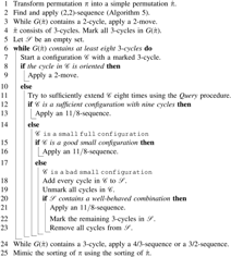
\end{document} and the undirected desire edges D = {(+i, −(i + 1)) |i = 0, … ,n}). Figure 1 shows \documentclass{aastex}\usepackage{amsbsy}\usepackage{amsfonts}\usepackage{amssymb}\usepackage{bm}\usepackage{mathrsfs}\usepackage{pifont}\usepackage{stmaryrd}\usepackage{textcomp}\usepackage{portland, xspace}\usepackage{amsmath, amsxtra}\pagestyle{empty}\DeclareMathSizes{10}{9}{7}{6}\begin{document}
$$G([{\bf{0}}\, 10\, 9\, 8\, 7\, 1\, 6\, 11\, 5\, 4\, 3\, 2\, \bf{12}])$$
\end{document}, where the arrows represent the directed edges in R and the arcs represent the undirected edges in D.
\documentclass{aastex}\usepackage{amsbsy}\usepackage{amsfonts}\usepackage{amssymb}\usepackage{bm}\usepackage{mathrsfs}\usepackage{pifont}\usepackage{stmaryrd}\usepackage{textcomp}\usepackage{portland, xspace}\usepackage{amsmath, amsxtra}\pagestyle{empty}\DeclareMathSizes{10}{9}{7}{6}\begin{document}
$$G([{\bf{0}}\, 10\, 9\, 8\, 7\, 1\, 6\, 11\, 5\, 4\, 3\, 2\, \bf{12}])$$
\end{document}. The set of cycles is {C1 = 〈024〉, C2 = 〈136〉, C3 = 〈5810〉, C4 = 〈7911〉}. The cycles C2 and C3 intersect, but are not interleaving; the cycles C1 and C2 are interleaving, and so are C3 and C4. The cycle C1 is the leftmost cycle.
Since every vertex in G(π) has degree 2, the graph can be partitioned into disjoint cycles. We shall use the terms a cycle in π and a cycle in G(π) interchangeably to denote the latter. A cycle in π has length ℓ (or it is an ℓ-cycle), if it has exactly ℓ reality edges. A permutation π is a simple permutation if every cycle in π has length at most 3, as the example in Figure 1.
After applying a transposition t, the number of cycles of odd length in G(π), denoted codd(π), changes in such a way that codd(π · t) = codd(π) + x, where x ∈ {−2, 0, 2}; the transposition t is thus classified as an x-move for π. Since codd(ι) = n + 1, we have the lower bound \documentclass{aastex}\usepackage{amsbsy}\usepackage{amsfonts}\usepackage{amssymb}\usepackage{bm}\usepackage{mathrsfs}\usepackage{pifont}\usepackage{stmaryrd}\usepackage{textcomp}\usepackage{portland, xspace}\usepackage{amsmath, amsxtra}\pagestyle{empty}\DeclareMathSizes{10}{9}{7}{6}\begin{document}
$$d ( \pi ) \ge \left[ \frac { ( n + 1 ) - c_ { odd } ( \pi ) } { 2 } \right]$$
\end{document}, where the equality holds if, and only if, π can be sorted solely with 2-moves.
Hannenhalli and Pevzner (1999) proved that every permutation π can be transformed, in O(n) time, into a simple one \documentclass{aastex}\usepackage{amsbsy}\usepackage{amsfonts}\usepackage{amssymb}\usepackage{bm}\usepackage{mathrsfs}\usepackage{pifont}\usepackage{stmaryrd}\usepackage{textcomp}\usepackage{portland, xspace}\usepackage{amsmath, amsxtra}\pagestyle{empty}\DeclareMathSizes{10}{9}{7}{6}\begin{document}
$$\hat{ \pi}$$
\end{document}, by inserting new elements in appropriate positions of π, preserving the lower bound for the distance, \documentclass{aastex}\usepackage{amsbsy}\usepackage{amsfonts}\usepackage{amssymb}\usepackage{bm}\usepackage{mathrsfs}\usepackage{pifont}\usepackage{stmaryrd}\usepackage{textcomp}\usepackage{portland, xspace}\usepackage{amsmath, amsxtra}\pagestyle{empty}\DeclareMathSizes{10}{9}{7}{6}\begin{document}
$$\left[ \frac { ( n + 1 ) - c_ { odd } ( \pi ) } { 2 } \right]
= \left[ \frac { ( m + 1 ) - c_ { odd } ( \hat { \pi } ) } { 2 }
\right]$$
\end{document}, where m is such that \documentclass{aastex}\usepackage{amsbsy}\usepackage{amsfonts}\usepackage{amssymb}\usepackage{bm}\usepackage{mathrsfs}\usepackage{pifont}\usepackage{stmaryrd}\usepackage{textcomp}\usepackage{portland, xspace}\usepackage{amsmath, amsxtra}\pagestyle{empty}\DeclareMathSizes{10}{9}{7}{6}\begin{document}
$$\hat{ \pi} = [{\bf 0}\hat{ \pi_1 }..\hat{ \pi_m} \bf {m+1}]$$
\end{document}. Additionally, in a sequence that sorts \documentclass{aastex}\usepackage{amsbsy}\usepackage{amsfonts}\usepackage{amssymb}\usepackage{bm}\usepackage{mathrsfs}\usepackage{pifont}\usepackage{stmaryrd}\usepackage{textcomp}\usepackage{portland, xspace}\usepackage{amsmath, amsxtra}\pagestyle{empty}\DeclareMathSizes{10}{9}{7}{6}\begin{document}
$$\hat{ \pi}$$
\end{document}, every transposition can be transformed, in O(logn) time (Feng and Zhu, 2007), into a sequence with the same number of transpositions that sorts π, which implies that \documentclass{aastex}\usepackage{amsbsy}\usepackage{amsfonts}\usepackage{amssymb}\usepackage{bm}\usepackage{mathrsfs}\usepackage{pifont}\usepackage{stmaryrd}\usepackage{textcomp}\usepackage{portland, xspace}\usepackage{amsmath, amsxtra}\pagestyle{empty}\DeclareMathSizes{10}{9}{7}{6}\begin{document}
$$d ( \pi ) \le d ( \hat{ \pi} )$$
\end{document}. The approach of finding a sorting sequence for π via a simple permutation \documentclass{aastex}\usepackage{amsbsy}\usepackage{amsfonts}\usepackage{amssymb}\usepackage{bm}\usepackage{mathrsfs}\usepackage{pifont}\usepackage{stmaryrd}\usepackage{textcomp}\usepackage{portland, xspace}\usepackage{amsmath, amsxtra}\pagestyle{empty}\DeclareMathSizes{10}{9}{7}{6}\begin{document}
$$\hat{ \pi}$$
\end{document} is commonly used in approximation algorithms for SBT (Elias and Hartman, 2006; Hartman and Shamir, 2006).
A transposition t (i, j, k) affects a cycle C if it contains one of the following reality edges: \documentclass{aastex}\usepackage{amsbsy}\usepackage{amsfonts}\usepackage{amssymb}\usepackage{bm}\usepackage{mathrsfs}\usepackage{pifont}\usepackage{stmaryrd}\usepackage{textcomp}\usepackage{portland, xspace}\usepackage{amsmath, amsxtra}\pagestyle{empty}\DeclareMathSizes{10}{9}{7}{6}\begin{document}
$$\overrightarrow{i + 1}$$
\end{document}, or \documentclass{aastex}\usepackage{amsbsy}\usepackage{amsfonts}\usepackage{amssymb}\usepackage{bm}\usepackage{mathrsfs}\usepackage{pifont}\usepackage{stmaryrd}\usepackage{textcomp}\usepackage{portland, xspace}\usepackage{amsmath, amsxtra}\pagestyle{empty}\DeclareMathSizes{10}{9}{7}{6}\begin{document}
$$\overrightarrow{j + 1}$$
\end{document}, or \documentclass{aastex}\usepackage{amsbsy}\usepackage{amsfonts}\usepackage{amssymb}\usepackage{bm}\usepackage{mathrsfs}\usepackage{pifont}\usepackage{stmaryrd}\usepackage{textcomp}\usepackage{portland, xspace}\usepackage{amsmath, amsxtra}\pagestyle{empty}\DeclareMathSizes{10}{9}{7}{6}\begin{document}
$$\overrightarrow{k + 1}$$
\end{document}. A cycle is oriented if there is a 2-move that affects it, otherwise it is unoriented (these names come from the order of such triplet of reality edges in the breakpoint graph). If π contains an oriented cycle then π is oriented, otherwise π is unoriented.
A sequence of q transpositions of which exactly r transpositions are 2-moves is a (q,r)-sequence. A q/r-sequence is an (x,y)-sequence such that x ≤ q and x/y ≤ q/r.
Interactions between cycles A cycle in π can be uniquely identified by its reality edges, in the order that they appear, starting from the leftmost edge. The notation C = 〈x1x2 … xℓ〉, where \documentclass{aastex}\usepackage{amsbsy}\usepackage{amsfonts}\usepackage{amssymb}\usepackage{bm}\usepackage{mathrsfs}\usepackage{pifont}\usepackage{stmaryrd}\usepackage{textcomp}\usepackage{portland, xspace}\usepackage{amsmath, amsxtra}\pagestyle{empty}\DeclareMathSizes{10}{9}{7}{6}\begin{document}
$$\overrightarrow{x_1}$$
\end{document}, \documentclass{aastex}\usepackage{amsbsy}\usepackage{amsfonts}\usepackage{amssymb}\usepackage{bm}\usepackage{mathrsfs}\usepackage{pifont}\usepackage{stmaryrd}\usepackage{textcomp}\usepackage{portland, xspace}\usepackage{amsmath, amsxtra}\pagestyle{empty}\DeclareMathSizes{10}{9}{7}{6}\begin{document}
$$\overrightarrow{x_2} , \ldots , \overrightarrow{x_{\ell}}$$
\end{document} are reality edges, and x1 = min {x1, x2, … ,xℓ}, characterizes an ℓ-cycle. The leftmost cycle is the cycle that contains the edge \documentclass{aastex}\usepackage{amsbsy}\usepackage{amsfonts}\usepackage{amssymb}\usepackage{bm}\usepackage{mathrsfs}\usepackage{pifont}\usepackage{stmaryrd}\usepackage{textcomp}\usepackage{portland, xspace}\usepackage{amsmath, amsxtra}\pagestyle{empty}\DeclareMathSizes{10}{9}{7}{6}\begin{document}
$$\overrightarrow{0}$$
\end{document}.
Let \documentclass{aastex}\usepackage{amsbsy}\usepackage{amsfonts}\usepackage{amssymb}\usepackage{bm}\usepackage{mathrsfs}\usepackage{pifont}\usepackage{stmaryrd}\usepackage{textcomp}\usepackage{portland, xspace}\usepackage{amsmath, amsxtra}\pagestyle{empty}\DeclareMathSizes{10}{9}{7}{6}\begin{document}
$$\overrightarrow{x} , \overrightarrow{y} , \overrightarrow{z}$$
\end{document}, where x < y < z, be reality edges in a cycle C, and \documentclass{aastex}\usepackage{amsbsy}\usepackage{amsfonts}\usepackage{amssymb}\usepackage{bm}\usepackage{mathrsfs}\usepackage{pifont}\usepackage{stmaryrd}\usepackage{textcomp}\usepackage{portland, xspace}\usepackage{amsmath, amsxtra}\pagestyle{empty}\DeclareMathSizes{10}{9}{7}{6}\begin{document}
$$\overrightarrow{a} , \overrightarrow{b} , \overrightarrow{c}$$
\end{document}, where a < b < c be reality edges in a different cycle C′. The pair of reality edges \documentclass{aastex}\usepackage{amsbsy}\usepackage{amsfonts}\usepackage{amssymb}\usepackage{bm}\usepackage{mathrsfs}\usepackage{pifont}\usepackage{stmaryrd}\usepackage{textcomp}\usepackage{portland, xspace}\usepackage{amsmath, amsxtra}\pagestyle{empty}\DeclareMathSizes{10}{9}{7}{6}\begin{document}
$$\overrightarrow{x} , \overrightarrow{y}$$
\end{document}, intersects the pair \documentclass{aastex}\usepackage{amsbsy}\usepackage{amsfonts}\usepackage{amssymb}\usepackage{bm}\usepackage{mathrsfs}\usepackage{pifont}\usepackage{stmaryrd}\usepackage{textcomp}\usepackage{portland, xspace}\usepackage{amsmath, amsxtra}\pagestyle{empty}\DeclareMathSizes{10}{9}{7}{6}\begin{document}
$$\overrightarrow{a}$$
\end{document}, \documentclass{aastex}\usepackage{amsbsy}\usepackage{amsfonts}\usepackage{amssymb}\usepackage{bm}\usepackage{mathrsfs}\usepackage{pifont}\usepackage{stmaryrd}\usepackage{textcomp}\usepackage{portland, xspace}\usepackage{amsmath, amsxtra}\pagestyle{empty}\DeclareMathSizes{10}{9}{7}{6}\begin{document}
$$\overrightarrow{b} ,$$
\end{document} if these four edges occur in an alternating order in the breakpoint graph, that is, either x < a < y < b or a < x < b < y, and we say C and C′ intersect. Similarly, a triplet of reality edges \documentclass{aastex}\usepackage{amsbsy}\usepackage{amsfonts}\usepackage{amssymb}\usepackage{bm}\usepackage{mathrsfs}\usepackage{pifont}\usepackage{stmaryrd}\usepackage{textcomp}\usepackage{portland, xspace}\usepackage{amsmath, amsxtra}\pagestyle{empty}\DeclareMathSizes{10}{9}{7}{6}\begin{document}
$$\overrightarrow{x} , \overrightarrow{y} , \overrightarrow{z}$$
\end{document}interleaves a triplet \documentclass{aastex}\usepackage{amsbsy}\usepackage{amsfonts}\usepackage{amssymb}\usepackage{bm}\usepackage{mathrsfs}\usepackage{pifont}\usepackage{stmaryrd}\usepackage{textcomp}\usepackage{portland, xspace}\usepackage{amsmath, amsxtra}\pagestyle{empty}\DeclareMathSizes{10}{9}{7}{6}\begin{document}
$$\overrightarrow{a} , \overrightarrow{b} , \overrightarrow{c}$$
\end{document} if these six edges occur in an alternating order: x < a < y < b < z < c or a < x < b < y < c < z. Two 3-cycles interleave if their respective triplets of reality edges interleave. Figure 1 also illustrates these concepts.
A configuration of π is a subset of the cycles in G(π). A configuration is connected if there is a sequence of C1, … ,Ck in such that C1 = C, Ck = C′ and for each i ∈ {1, 2, … , k − 1}, the cycles Ci and Ci+1 are intersecting. If the configuration is connected and maximal, then is a component. Every permutation admits a unique decomposition into disjoint components. For instance, in Figure 1, the configuration {C1, C2, C3, C4} is a component, but the configuration {C1, C2, C3} is connected but not a component.
Let C be a 3-cycle in configuration . An open gate is a pair of reality edges in C that does not intersect any other pair of reality edges in . If a configuration has only 3-cycles and no open gates, then is a full configuration. Some full configurations do not correspond to the breakpoint graph of any permutation. A full configuration corresponds to a permutation if, and only if, the complement configuration is Hamiltonian (Elias and Hartman, 2006), as illustrated in Figure 2b. Figure 2a shows the full configuration F = {〈0 7 9〉, 〈1 3 6〉, 〈2 4 11〉, 〈5 8 11〉}, which does not correspond to any permutation but is important in the analysis of our algorithm and will be studied in detail in section 5.
(a) Full configuration F = {〈079〉, 〈136〉, 〈2411〉, 〈5810〉}, which does not correspond to a permutation. (b) Complement of F, obtained by replacing the reality edges with the edges -πiπi and 0-πn+1.
A configuration that has k edges is in the cromulent form4 if all edges \documentclass{aastex}\usepackage{amsbsy}\usepackage{amsfonts}\usepackage{amssymb}\usepackage{bm}\usepackage{mathrsfs}\usepackage{pifont}\usepackage{stmaryrd}\usepackage{textcomp}\usepackage{portland, xspace}\usepackage{amsmath, amsxtra}\pagestyle{empty}\DeclareMathSizes{10}{9}{7}{6}\begin{document}
$$\overrightarrow{0} , \overrightarrow{1} , \ldots , \overrightarrow{k - 1}$$
\end{document} are in . Given a configuration having k edges, a cromulent relabeling of is a configuration such that is in the cromulent form and there is a function σ satisfying that, for every pair of edges \documentclass{aastex}\usepackage{amsbsy}\usepackage{amsfonts}\usepackage{amssymb}\usepackage{bm}\usepackage{mathrsfs}\usepackage{pifont}\usepackage{stmaryrd}\usepackage{textcomp}\usepackage{portland, xspace}\usepackage{amsmath, amsxtra}\pagestyle{empty}\DeclareMathSizes{10}{9}{7}{6}\begin{document}
$$\overrightarrow{i} , \overrightarrow{j}$$
\end{document}, in such that i < j, we have that \documentclass{aastex}\usepackage{amsbsy}\usepackage{amsfonts}\usepackage{amssymb}\usepackage{bm}\usepackage{mathrsfs}\usepackage{pifont}\usepackage{stmaryrd}\usepackage{textcomp}\usepackage{portland, xspace}\usepackage{amsmath, amsxtra}\pagestyle{empty}\DeclareMathSizes{10}{9}{7}{6}\begin{document}
$$\overrightarrow{ \sigma ( i ) } , \overrightarrow{ \sigma ( j ) }$$
\end{document}, are in and σ(i) < σ(j). For instance, in Figure 2a the cromulent relabeling of the configuration {C1 = 〈0, 7, 9〉, C2 = 〈1, 3, 6〉} is {C1 = 〈0, 4, 5〉, C2 = 〈1, 2, 3〉}.
Given an integer x, a circular shift of a configuration , which is in the cromulent form and has k edges, is a configuration denoted such that every edge \documentclass{aastex}\usepackage{amsbsy}\usepackage{amsfonts}\usepackage{amssymb}\usepackage{bm}\usepackage{mathrsfs}\usepackage{pifont}\usepackage{stmaryrd}\usepackage{textcomp}\usepackage{portland, xspace}\usepackage{amsmath, amsxtra}\pagestyle{empty}\DeclareMathSizes{10}{9}{7}{6}\begin{document}
$$\overrightarrow{i}$$
\end{document} in corresponds to \documentclass{aastex}\usepackage{amsbsy}\usepackage{amsfonts}\usepackage{amssymb}\usepackage{bm}\usepackage{mathrsfs}\usepackage{pifont}\usepackage{stmaryrd}\usepackage{textcomp}\usepackage{portland, xspace}\usepackage{amsmath, amsxtra}\pagestyle{empty}\DeclareMathSizes{10}{9}{7}{6}\begin{document}
$$\overrightarrow{i + x ( { \rm mod} \ k ) }$$
\end{document} in . Two configurations and are equivalent if there is an integer x such that , where and are their respective cromulent relabelings.
Elias and Hartman's algorithm Elias and Hartman (2006) performed a systematic enumeration of all components with nine cycles or less, in which all cycles have length 3. Starting from single 3-cycles, components were obtained by applying a series of sufficient extensions, as described next. An extension of a configuration is a connected configuration , where . A sufficient extension is an extension that either: 1) closes an open gate; or 2) extends a full configuration such that the extension has at most one open gate. A configuration obtained by a series of sufficient extensions is a sufficient configuration if an (x,y)-, or an x/y-sequence can be applied to its cycles.
Lemma 1(Elias and Hartman, 2006) Every unoriented sufficient configuration of nine cycles has an 11/8-sequence.
Components with less than nine cycles are called small components. Elias and Hartman have shown that, of all small components, only five types of them do not have an 11/8-sequence; these components are called bad small components. Small components that have an 11/8-sequence are called good small components.
Lemma 2(Elias and Hartman, 2006) The bad small components are:
• A = {〈0 2 4〉, 〈1 3 5〉};
• B = {〈0 2 10〉, 〈1 3 5〉, 〈4 6 8〉, 〈7 9 11〉};
• C = {〈0 5 7〉, 〈1 9 11〉, 〈2 4 6〉, 〈3 8 10〉};
• D = {〈0 2 4〉, 〈1 12 14〉, 〈3 5 7〉, 〈6 8 10〉,〈9 11 13〉}; and
If a permutation has bad small components, it is still possible to find an (11,8)-sequence, as Lemma 3 states.
Lemma 3(Elias and Hartman, 2006) Let π be a permutation with at least eight cycles and containing only bad small components. Then π has an (11,8)-sequence.
Corollary 1(Elias and Hartman, 2006) If every cycle in G(π) is a 3-cycle, and there are at least eight cycles, then π has an 11/8-sequence.
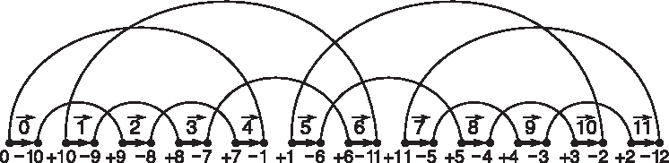
Lemmas 1 and 3 and Corollary 1 form the theoretical basis for Elias and Hartman's 11/8 = 1.375-approximation algorithm for SBT, Algorithm 1. The main procedure of Algorithm 1 is: obtain extensions, if a configuration with nine cycles or if a small good component is reached, then an 11/8-sequence is applied (Lemma 1); if a bad small component is reached then no sequence is applied. After all configurations with nine cycles or small good components have been sorted, the permutation just contains small bad components; Lemma 3 states the existence of an (11,8)-sequence.
Elias and Hartman's Sort(π)
Feng and Zhu's permutation tree Feng and Zhu (2007) introduced the permutation tree, a binary balanced tree that represents a permutation. In logarithmic time the operation of applying a transposition could be done, and also the Query procedure of finding a pair of reality edges that intersects another given pair of reality edges, as well. The Query procedure is the method used in Hartman and Shamir's (2006) 1.5-approximation algorithm to find a (3,2)-sequence that affects a pair of intersecting or interleaving cycles. Besides that, Firoz et al. (2011) claimed the Query procedure could be used to sufficiently extend a configuration in Algorithm 1.
Let \documentclass{aastex}\usepackage{amsbsy}\usepackage{amsfonts}\usepackage{amssymb}\usepackage{bm}\usepackage{mathrsfs}\usepackage{pifont}\usepackage{stmaryrd}\usepackage{textcomp}\usepackage{portland, xspace}\usepackage{amsmath, amsxtra}\pagestyle{empty}\DeclareMathSizes{10}{9}{7}{6}\begin{document}
$$\pi = [{\bf \pi}_{\bf 0} \pi_1 \pi_2 \ldots \pi_n {\bf \pi}_{n + 1}]$$
\end{document} be a permutation. The corresponding permutation tree has n leaves, labeled \documentclass{aastex}\usepackage{amsbsy}\usepackage{amsfonts}\usepackage{amssymb}\usepackage{bm}\usepackage{mathrsfs}\usepackage{pifont}\usepackage{stmaryrd}\usepackage{textcomp}\usepackage{portland, xspace}\usepackage{amsmath, amsxtra}\pagestyle{empty}\DeclareMathSizes{10}{9}{7}{6}\begin{document}
$$\pi_1 , \pi_2 , \ldots , \pi_n$$
\end{document}; every internal node represents an interval of consecutive elements \documentclass{aastex}\usepackage{amsbsy}\usepackage{amsfonts}\usepackage{amssymb}\usepackage{bm}\usepackage{mathrsfs}\usepackage{pifont}\usepackage{stmaryrd}\usepackage{textcomp}\usepackage{portland, xspace}\usepackage{amsmath, amsxtra}\pagestyle{empty}\DeclareMathSizes{10}{9}{7}{6}\begin{document}
$$\pi_i , \pi_{i + 1} , \ldots , \pi_{k - 1}$$
\end{document}, with i < k, and is labeled by the maximum number in the interval. Therefore, the root of the tree is labeled with n. Furthermore, the left child of a node represents the interval \documentclass{aastex}\usepackage{amsbsy}\usepackage{amsfonts}\usepackage{amssymb}\usepackage{bm}\usepackage{mathrsfs}\usepackage{pifont}\usepackage{stmaryrd}\usepackage{textcomp}\usepackage{portland, xspace}\usepackage{amsmath, amsxtra}\pagestyle{empty}\DeclareMathSizes{10}{9}{7}{6}\begin{document}
$$\pi_i , \ldots , \pi_{j - 1}$$
\end{document}, and the right child represents \documentclass{aastex}\usepackage{amsbsy}\usepackage{amsfonts}\usepackage{amssymb}\usepackage{bm}\usepackage{mathrsfs}\usepackage{pifont}\usepackage{stmaryrd}\usepackage{textcomp}\usepackage{portland, xspace}\usepackage{amsmath, amsxtra}\pagestyle{empty}\DeclareMathSizes{10}{9}{7}{6}\begin{document}
$$\pi_j , \ldots , \pi_k$$
\end{document}, with i < j < k. Feng and Zhu provided algorithms: to build a permutation tree in O(n) time; to join two permutation trees into one in O(h) time, where h is the height difference between the trees; and to split a permutation tree into two in O(logn) time.
The operations split and join allow us to apply a transposition to a permutation π, updating the tree, in time O(logn). Based on Lemma 4, the Query procedure (Algorithm 2) solves the problem of finding a pair of reality edges intersecting another given pair of reality edges.
Lemma 4(Bafna and Pevzner, 1998) Let\documentclass{aastex}\usepackage{amsbsy}\usepackage{amsfonts}\usepackage{amssymb}\usepackage{bm}\usepackage{mathrsfs}\usepackage{pifont}\usepackage{stmaryrd}\usepackage{textcomp}\usepackage{portland, xspace}\usepackage{amsmath, amsxtra}\pagestyle{empty}\DeclareMathSizes{10}{9}{7}{6}\begin{document}
$$\overrightarrow{i}$$
\end{document}and\documentclass{aastex}\usepackage{amsbsy}\usepackage{amsfonts}\usepackage{amssymb}\usepackage{bm}\usepackage{mathrsfs}\usepackage{pifont}\usepackage{stmaryrd}\usepackage{textcomp}\usepackage{portland, xspace}\usepackage{amsmath, amsxtra}\pagestyle{empty}\DeclareMathSizes{10}{9}{7}{6}\begin{document}
$$\overrightarrow{j}$$
\end{document}be two reality edges in an unoriented cycle C, i < j. Let πk = maxi<m≤jπm, πℓ = πk + 1. Then, the reality edges\documentclass{aastex}\usepackage{amsbsy}\usepackage{amsfonts}\usepackage{amssymb}\usepackage{bm}\usepackage{mathrsfs}\usepackage{pifont}\usepackage{stmaryrd}\usepackage{textcomp}\usepackage{portland, xspace}\usepackage{amsmath, amsxtra}\pagestyle{empty}\DeclareMathSizes{10}{9}{7}{6}\begin{document}
$$\overrightarrow{k}$$
\end{document}and\documentclass{aastex}\usepackage{amsbsy}\usepackage{amsfonts}\usepackage{amssymb}\usepackage{bm}\usepackage{mathrsfs}\usepackage{pifont}\usepackage{stmaryrd}\usepackage{textcomp}\usepackage{portland, xspace}\usepackage{amsmath, amsxtra}\pagestyle{empty}\DeclareMathSizes{10}{9}{7}{6}\begin{document}
$$\overrightarrow{\ell - 1}$$
\end{document}belong to the same cycle, and the pair\documentclass{aastex}\usepackage{amsbsy}\usepackage{amsfonts}\usepackage{amssymb}\usepackage{bm}\usepackage{mathrsfs}\usepackage{pifont}\usepackage{stmaryrd}\usepackage{textcomp}\usepackage{portland, xspace}\usepackage{amsmath, amsxtra}\pagestyle{empty}\DeclareMathSizes{10}{9}{7}{6}\begin{document}
$$\overrightarrow{k} , \overrightarrow{\ell - 1}$$
\end{document}intersects pair\documentclass{aastex}\usepackage{amsbsy}\usepackage{amsfonts}\usepackage{amssymb}\usepackage{bm}\usepackage{mathrsfs}\usepackage{pifont}\usepackage{stmaryrd}\usepackage{textcomp}\usepackage{portland, xspace}\usepackage{amsmath, amsxtra}\pagestyle{empty}\DeclareMathSizes{10}{9}{7}{6}\begin{document}
$$\overrightarrow{i} , \overrightarrow{j}$$
\end{document}.
Let πk = root (T2). (the largest element in the interval \documentclass{aastex}\usepackage{amsbsy}\usepackage{amsfonts}\usepackage{amssymb}\usepackage{bm}\usepackage{mathrsfs}\usepackage{pifont}\usepackage{stmaryrd}\usepackage{textcomp}\usepackage{portland, xspace}\usepackage{amsmath, amsxtra}\pagestyle{empty}\DeclareMathSizes{10}{9}{7}{6}\begin{document}
$$\pi_{i + 1} , \ldots , \pi_J$$
\end{document})
4
Let \documentclass{aastex}\usepackage{amsbsy}\usepackage{amsfonts}\usepackage{amssymb}\usepackage{bm}\usepackage{mathrsfs}\usepackage{pifont}\usepackage{stmaryrd}\usepackage{textcomp}\usepackage{portland, xspace}\usepackage{amsmath, amsxtra}\pagestyle{empty}\DeclareMathSizes{10}{9}{7}{6}\begin{document}
$$\pi_\ell = \pi_k + 1$$
\end{document}
Firoz et al. (2011) suggested the use of the permutation tree data structure to reduce the running time of Algorithm 1 to O(nlogn), but in section 3 we show that the strategy, in the manner proposed by Firoz et al., fails to extend some 3-cycles into a full configuration with nine cycles.
3. The Use of the Permutation Tree by Firoz et al.
Firoz et al. (2011) stated that Step 9 in Algorithm 1 could be done in O(logn) time. To do so, they categorized the sufficient extensions of a configuration A obtained by a Query call into type 1 extensions—those that add a cycle that closes an open gate—and type 2 extensions—those that extend a full configuration by adding a cycle C such that A ∪ {C} has at most one open gate.
A type 1 extension can be performed in logarithmic time with Query(π, i, j), where \documentclass{aastex}\usepackage{amsbsy}\usepackage{amsfonts}\usepackage{amssymb}\usepackage{bm}\usepackage{mathrsfs}\usepackage{pifont}\usepackage{stmaryrd}\usepackage{textcomp}\usepackage{portland, xspace}\usepackage{amsmath, amsxtra}\pagestyle{empty}\DeclareMathSizes{10}{9}{7}{6}\begin{document}
$$\overrightarrow{i} , \overrightarrow{j}$$
\end{document} form an open gate. For a type 2 extension, since there are no open gates, Firoz et al. claimed that it would be sufficient to perform queries with every pair of reality edges that belonged to the same cycle in the configuration that is being extended. Example 1 shows that this strategy is flawed.
Example 1Consider the permutation π = [0 10 9 8 7 1 6 11 5 4 3 2 12], whose breakpoint graph is depicted in Figure 1. It is a simple permutation having only unoriented 3-cycles. Mark all the cycles C1 = 〈0,2,4〉, C2 = 〈1, 3, 6〉, C3 = 〈5,8,10〉, and C4 = 〈7,9,11〉. Let A = {C1}be the configuration to be sufficiently extended (step 9 in Algorithm 1). Using the method proposed by Firoz et al., we have that:
1. Configuration A has three open gates\documentclass{aastex}\usepackage{amsbsy}\usepackage{amsfonts}\usepackage{amssymb}\usepackage{bm}\usepackage{mathrsfs}\usepackage{pifont}\usepackage{stmaryrd}\usepackage{textcomp}\usepackage{portland, xspace}\usepackage{amsmath, amsxtra}\pagestyle{empty}\DeclareMathSizes{10}{9}{7}{6}\begin{document}
$$\overrightarrow{0} , \overrightarrow{2}{\rm;}
\overrightarrow{2} , \overrightarrow{4}{\rm;} \overrightarrow{4} ,
\overrightarrow{0}$$
\end{document}. Execute Query(π, 0, 2), which returns the pair\documentclass{aastex}\usepackage{amsbsy}\usepackage{amsfonts}\usepackage{amssymb}\usepackage{bm}\usepackage{mathrsfs}\usepackage{pifont}\usepackage{stmaryrd}\usepackage{textcomp}\usepackage{portland, xspace}\usepackage{amsmath, amsxtra}\pagestyle{empty}\DeclareMathSizes{10}{9}{7}{6}\begin{document}
$$\overrightarrow{1} , \overrightarrow{6}$$
\end{document}, in cycle C2 = 〈1, 3, 6〉 (or, alternatively Query(π, 2, 4), which yields the same result). Therefore, C2is added to the configuration A, which becomes A = {C1, C2}.
2. Configuration A has no more open gates. We must execute Query(π,i,j) for every pair of elements\documentclass{aastex}\usepackage{amsbsy}\usepackage{amsfonts}\usepackage{amssymb}\usepackage{bm}\usepackage{mathrsfs}\usepackage{pifont}\usepackage{stmaryrd}\usepackage{textcomp}\usepackage{portland, xspace}\usepackage{amsmath, amsxtra}\pagestyle{empty}\DeclareMathSizes{10}{9}{7}{6}\begin{document}
$$\overrightarrow{i} , \overrightarrow{j}$$
\end{document}in the same cycle of the configuration such that i < j; it is easy to observe that each execution returns a pair that is already in A. So far, Firozet al.'s method has failed to extend A.
3. Since A is not a component, unmark all the cycles in A.
4. The marked cycles are now C3and C4. Considering either A = {C3} or A = {C4},Firoz et al.'s method only extends A as far as {C3, C4}. Again, A is not a component.
Therefore, Firoz et al.'s method fails to find the component{C1, C2, C3, C4}.
Although the permutation in Example 1 has only one small component, it is a counterexample to the correctness of Firoz et al.'s strategy for dealing with type 2 extensions. The same problem happens for sufficient configurations with more than nine cycles, such as:
\documentclass{aastex}\usepackage{amsbsy}\usepackage{amsfonts}\usepackage{amssymb}\usepackage{bm}\usepackage{mathrsfs}\usepackage{pifont}\usepackage{stmaryrd}\usepackage{textcomp}\usepackage{portland, xspace}\usepackage{amsmath, amsxtra}\pagestyle{empty}\DeclareMathSizes{10}{9}{7}{6}\begin{document}
\begin{align*}{\rm \sigma} = [ { \bf 0} \ 25 \ 24 \ 23 \ 22 \ 1 \
21 \ 26 \ 20 \ 19 \ 18 \ 2 \ 17 \ 27 \ 16 \ 15 \ 14 \ 3 \ 13 \ 28
\ 12 \ 11 \ 10 \ 4 \ 9 \ 29 \ 8 \ 7 \ 6 \ 5 \ { \bf 30}
].\end{align*}
\end{document}
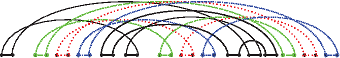
By Lemma 1, every configuration of nine cycles has an 11/8-sequence. Figure 3 shows an example of a breakpoint graph of σ with 10 cycles, for which any configuration with 9 cycles has an 11/8-sequence. However, Firoz et al.'s approach fails to find such a sequence, for it performs the following sequence of operations: i) starting from any configuration having a unique cycle, the first call to Query correctly finds another intersecting cycle, which is added to the configuration (Fig. 4); ii) with this configuration having two interleaving cycles, every possible invocation of Query returns one of the cycles already in the configuration, which means that their strategy cannot further extend the configuration; iii) the resulting configuration, with only two cycles, is a bad small component, so the cycles are unmarked; iv) if an unmarked cycle still remains, it is selected to start a configuration, and we return to the first step in this sequence of operations. The procedure finishes after unmarking all 10 cycles, incorrectly presuming that the breakpoint graph only has bad small components with two cycles.
Breakpoint graph of a permutation σ for which Firoz et al.'s method fails. Note that σ has 10 cycles, and that σ is obtained by setting k = 5 in Equation (2).
A configuration that is not maximal returned by a Query call on σ.
Notice that, according to Step 18 in Algorithm 1, if a permutation contains only bad small components, then an 11/8-sequence can be applied. The permutation γ (whose breakpoint graph is in Fig. 5) is one of those permutations:
\documentclass{aastex}\usepackage{amsbsy}\usepackage{amsfonts}\usepackage{amssymb}\usepackage{bm}\usepackage{mathrsfs}\usepackage{pifont}\usepackage{stmaryrd}\usepackage{textcomp}\usepackage{portland, xspace}\usepackage{amsmath, amsxtra}\pagestyle{empty}\DeclareMathSizes{10}{9}{7}{6}\begin{document}
\begin{align*}\gamma = [ { \bf 0} \ 5 \ 4 \ 3 \ 2 \ 1 \ 6 \ 11 \
10 \ 9 \ 8 \ 7 \ 12 \ 17 \ 16 \ 15 \ 14 \ 13 \ 18 \ 23 \ 22 \ 21 \
20 \ 19 \ 24 \ 29 \ 28 \ 27 \ 26 \ 25 \ { \bf 30} ] ,\end{align*}
\end{document}
Notice how the breakpoint graphs in Figures 4 and 5 differ, but according to Firoz et al.'s approach they would be indistinguishable. In Figure 5, the bad small components can be separately handled, which is not the case for configurations with two interleaving cycles in Figure 4, for these configurations intersect other cycles. Algorithm 1 does not have a rule to deal with this last case.
The breakpoint graph of permutation γ.
Note that the permutation of Example 1 and the permutation above σ just describe examples belonging to a family of permutations such that any type 2 extension fails. Actually, an infinite family can be constructed as follows: let k be any integer greater than or equal to 2, and let f (i) be the sequence of six integers
\documentclass{aastex}\usepackage{amsbsy}\usepackage{amsfonts}\usepackage{amssymb}\usepackage{bm}\usepackage{mathrsfs}\usepackage{pifont}\usepackage{stmaryrd}\usepackage{textcomp}\usepackage{portland, xspace}\usepackage{amsmath, amsxtra}\pagestyle{empty}\DeclareMathSizes{10}{9}{7}{6}\begin{document}
\begin{align*}i \ 5k - 4i \ 5k + i \ 5k - 4i - 1 \ 5k - 4i - 2 \
5k - 4i - 3. \tag{\rm 1}\end{align*}
\end{document}
Consider σk a permutation of 6k − 1 elements defined using Equation (1) as:
\documentclass{aastex}\usepackage{amsbsy}\usepackage{amsfonts}\usepackage{amssymb}\usepackage{bm}\usepackage{mathrsfs}\usepackage{pifont}\usepackage{stmaryrd}\usepackage{textcomp}\usepackage{portland, xspace}\usepackage{amsmath, amsxtra}\pagestyle{empty}\DeclareMathSizes{10}{9}{7}{6}\begin{document}
\begin{align*}[ { \bf 0} \ 5k \ 5k - 1 \ 5k - 2 \ 5k - 3 \ f ( 1
) \ f ( 2 ) \ldots \ f ( k - 1 ) \ k \ { \bf 6k} ] , \tag{\rm
2}\end{align*}
\end{document}
whose breakpoint graph has a similar structure to those in Figure 1 (where in Equation (2) we set k = 2) and 3. If we start from a configuration having any cycle, it is impossible to extend it past a configuration of more than two cycles using Firoz et al.'s approach.
Some other configurations cannot be extended using only the Query procedure either, such as the full configuration illustrated in Figure 2. This is a bad small configuration (Elias and Hartman, 2006) that does not correspond to the breakpoint graph of any permutation, but this configuration may appear during the sorting of a larger permutation.
4. Finding and Applying A (2,2)-Sequence in Linear Time
In order to implement Step 2 of Algorithm 1, Elias and Hartman (2006) proved that, given a simple permutation, a (2,2)-sequence can be found in O(n2) time.
Firoz et al. (2011) described a strategy for finding and applying a (2,2)-sequence in O(nlogn) time using permutation trees. But, according to their strategy, for each one of the O(n) oriented 3-cycles, we apply a 2-move and check in O(n) time for the existence of an oriented cycle in the resulting graph, which implies that Firoz et al.'s strategy may run in Ω(n2) time in the worst case. One such case is illustrated in Figure 6, where the cycles drawn in solid lines—one oriented, the other unoriented—are interleaving, so by case 3 of Lemma 5 there is a (2,2)-sequence that affects them. However, if the first 2-move is applied to any of the dashed cycles, the resulting breakpoint graph has no oriented cycle, hence the transposition is undone and another oriented cycle is selected; this procedure would continue until the solid oriented cycle is selected.
A breakpoint graph for which Firoz et al.'s strategy takes Ω(n2) time in the worst case to find a (2,2)-sequence.
Algorithm 5 summarizes our proposed approach toward finding and applying a (2,2)-sequence in O(n) time. It is a direct application of Algorithms 3 and 4 to the cases stated in Lemma 5.
Search (2,2)-sequence from K1.
Lemma 5(Bafna and Pevzner, 1998; Christie, 1999; Elias and Hartman, 2006) Given a breakpoint graph of a simple permutation, there exists a (2,2)-sequence if any of the following conditions is met:
1. There are either four 2-cycles, or two intersecting 2-cycles, or two nonintersecting 2-cycles, and the resulting graph contains an oriented cycle after the first transposition is applied;
2. There are two noninterleaving oriented 3-cycles;
3. There is an oriented cycle interleaving an unoriented cycle.
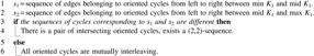
Our strategy to find a (2,2)-sequence in linear time starts by checking whether the breakpoint graph satisfies first case of Lemma 5, as described in detail between lines 1 and 4 in Algorithm 5. In our approach, it is unnecessary to try all pairs of cycles to verify that conditions 2 and 3 in Lemma 5 are satisfied. It differs from previous methods (Elias and Hartman, 2006; Firoz et al., 2011) in that the leftmost oriented cycle of the breakpoint graph, named K1, is fixed when verifying for conditions 2 and 3.
Given a simple permutation π, it is immediate to enumerate all of its cycles in linear time. The size of each cycle, and whether it is oriented, are both determined in constant time.
Christie (1999) proved that every permutation has an even number (possibly zero) of even cycles; he also showed that, given a simple permutation, when the number of even cycles is not zero, there exists a (2,2)-sequence that affects those cycles if, and only if, there are either four 2-cycles, or there are two intersecting even cycles. Therefore, in these cases, a (2,2)-sequence can be applied in O(logn) using permutation trees. If there is only a pair of nonintersecting 2-cycles, it remains to check if there is a 3-cycle intersecting both even cycles: i) if the 3-cycle is oriented, then first we apply the 2-move applied to the 3-cycle, and the second 2-move is applied to 2-cycles; ii) if the 3-cycle is unoriented, then first we apply the 2-move applied to the 2-cycles, and the second 2-move is applied to the 3-cycle, which turns oriented after the first transposition. There is also a (2,2)-sequence if there is an oriented cycle intersecting at most one even cycle.
However, if there are no even cycles in the permutation, but there is an oriented cycle, the 3-cycles must be scanned for the existence of a (2,2)-sequence, as conditions 2 and 3 require in Lemma 5.
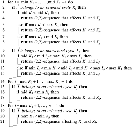
To check, in linear time, for the existence of a pair of cycles satisfying either condition 2 or 3 in Lemma 5, consider the oriented cycles of the breakpoint graph, in the order K1 = 〈a1b1c1〉, K2 = 〈a2b2c2〉, K3 = 〈a3b3c3〉, … such that a1 < a2 < a3 < … , and the unoriented cycles in the order L1 = 〈x1y1z1〉, L2 = 〈x2y2z2〉, L3 = 〈x3y3z3〉, … such that x1 < x2 < x3 < … . Given any 3-cycle C = 〈abc〉, let min C = a, mid C = min {b,c}, and max C = max {b,c}, that is, if C is unoriented, then min C = a, mid C = b, max C = c, whereas if C is oriented, then min C = a, mid C = c, max C = b. The main idea is:
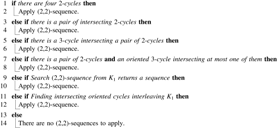
1. Check for the existence of an oriented cycle Kj noninterleaving K1 or an unoriented cycle Lj interleaving K1. Algorithm 3 searches for an oriented cycle Ki noninterleaving K1 or an unoriented cycle Li interleaving K1. The search is done between minK1 and mid K1, between mid K1 and max K1, and to the right of max K1.
2. If Algorithm 3 does not return any oriented cycle noninterleaving K1, then every oriented cycle interleaves K1 but no unoriented cycle interleaves K1. Hence, we must check for the existence of two oriented cycles Ki, Kj that are intersecting but not interleaving. Note that if Ki, Kj were nonintersecting oriented cycles, Algorithm 3 would have this case already covered (see Fig. 7), since Ki or Kj would not interleave K1. Algorithm 4 describes how to verify the existence of two intersecting oriented cycles that are also interleaving with K1.
Find and Apply (2,2)-sequence
Oriented cycles represented by their reality edges. All oriented cycles interleave K1, but there are i and j such that Ki and Kj are noninterleaving.
5. Sufficient Extensions Using the Query Procedure
In section 3, we discussed Firoz et al.'s use of the permutation tree and proved that their strategy does not account for every configuration with less than nine cycles that is not a component, since successive invocations of Query may result in a full configuration with less than nine cycles that is not a small component. Our proposed strategy generalizes the definitions regarding small components to small configurations—configurations with less than nine cycles.
A small configuration is full if it has no open gates. Small configurations are also classified as good if they have an 11/8-sequence, or as bad otherwise.
Algorithm 1 applies an 11/8-sequence to every sufficient unoriented configuration of nine cycles, and also to every good small component. After that, the permutation contains just bad small components, and Lemma 3 states that there exists an (11,8)-sequence for every combination of bad small components with at least eight cycles.
Our approach can handle bad small full configurations, which may or may not be bad small components, during the course of an extension via successive invocations of Query. The possible bad small full configurations are the bad small components A, B, C, D, and E, from Lemma 2, and the full configuration F = {〈079〉, 〈136〉, 〈2411〉, 〈5810〉}, the only bad small full configuration that is not a component (Elias and Hartman, 2006).
Our strategy (Algorithm 6) is similar to Elias and Hartman's (Algorithm 1): apply an 11/8-sequence to every sufficient unoriented configuration of nine cycles and also to every good small full configuration; the main difference is that, whenever a combination of bad small full configurations is found, a decision to apply an 11/8-sequence is made according to Lemmas 6 and 7.
We developed a tool (Cunha et al., 2014a) that finds 11/8-sequences for a given configuration using branch-and-bound, where a branch is obtained by either applying a 2-move or a 0-move, and the moves are bounded by the ratio between the number of total moves and the number of 2-moves, which cannot be greater than 1.375. The algorithm either returns an 11/8-sequence, whenever it exists, or fails after trying all possible sequences.
Lemma 6Every combination of F with one or more copies of either B, C, D, or E has an 11/8-sequence.
Proof. Consider all breakpoint graphs of F and its circular shifts combined with B, C, D, E, and their circular shifts. A combination of a pair of small full configurations is obtained by starting from one small full configuration and inserting a new one in different positions in the breakpoint graph. Altogether, there are 324 such graphs. A computerized case analysis (Cunha et al., 2014a) enumerates all possible breakpoint graphs and provides an 11/8-sequence for each of them. ■
Notice that Lemma 6 considers neither combinations of F with F, nor combinations of F with A. We have found that almost every combination of F with F has an 11/8-sequence, as Lemma 7 states. Let FiFj be the configuration obtained by inserting the circular shift F + j between the edges \documentclass{aastex}\usepackage{amsbsy}\usepackage{amsfonts}\usepackage{amssymb}\usepackage{bm}\usepackage{mathrsfs}\usepackage{pifont}\usepackage{stmaryrd}\usepackage{textcomp}\usepackage{portland, xspace}\usepackage{amsmath, amsxtra}\pagestyle{empty}\DeclareMathSizes{10}{9}{7}{6}\begin{document}
$$\overrightarrow{i}$$
\end{document} and \documentclass{aastex}\usepackage{amsbsy}\usepackage{amsfonts}\usepackage{amssymb}\usepackage{bm}\usepackage{mathrsfs}\usepackage{pifont}\usepackage{stmaryrd}\usepackage{textcomp}\usepackage{portland, xspace}\usepackage{amsmath, amsxtra}\pagestyle{empty}\DeclareMathSizes{10}{9}{7}{6}\begin{document}
$$\overrightarrow{i + 1}$$
\end{document} of F.
Lemma 7There exists an 11/8-sequence for FiFj, if:
• i ∈ {0,4} and j ∈ {0,1,2,3,4,5};
• i ∈ {1,2,3} and j ∈ {1,2,3,4,5}; or
• i = 5 and j ∈ {1,5}.
Proof. The 11/8-sequences for the cases enumerated above were also found through a computerized case analysis (Cunha et al., 2014a). Note that FiFj is equivalent to Fi+6Fj for i = {0, 1, … ,5}, which simplifies our analysis. ■
Only seven combinations of F with F have no 11/8-sequence: F1F0, F2F0, F3F0, F5F0, F5F2, F5F3, and F5F4. We will return to them shortly.
All combinations of one copy of F and one copy of A have less than eight cycles. It only remains to analyze the combinations of F and two copies of A, denoted F–A–A. The good F–A–A combinations are the F–A–A combinations for which an 11/8-sequence exists. Out of 57 combinations of F–A–A, only 31 are good. The complete list of combinations is in Cunha et al. (2014a).
Combinations of F with A, B, C, D, E, and F that have 11/8-sequences are called well-behaved combinations—the ones in Lemmas 6, 7, and the good F–A–A combinations. The remaining combinations having F are called naughty: the seven combinations of F – F that have no 11/8-sequence, and the 57 combinations of F–A–A.
For extensions that yield a bad small configuration, Algorithm 6 adds their cycles to a set (line 32). Later, if a well-behaved combination is found among the cycles in , an 11/8-sequence is applied (line 37) and the set is emptied. If all combinations in are naughty, another bad small configuration can be obtained and added to it in the next iteration (line 6).
We have shown (Cunha et al., 2014a) that every combination of three copies of F is well-behaved, even if each pair of F – F is naughty; the same can be said of every combination of F and three copies of A, even if each triple F–A–A is naughty. Therefore, at most 12 cycles are in , since it may contain at most three copies of F, or one copy of F and three copies of A, in the worst case. For each of these cases, there exists an 11/8-sequence (Cunha et al., 2014a).
Proposed algorithmAlgorithm 6 is a direct application of the results in the section. In a nutshell, it obtains configurations using the Query procedure and applies 11/8-sequences to configurations of size at most 9. Algorithm 6 differs from Algorithm 1 not only in the use of permutation trees, but also because the main loop handles bad small full configurations, instead of only dealing with them at the end.
Proposed algorithm based on Elias and Hartman's algorithm
Proof. Steps 1 through 5 can be implemented to run in linear time [Elias and Hartman (2006); Feng and Zhu (2007), and section 4]. Step 17 runs in O(log n) time using permutation trees. The comparisons in Steps 12, 15, and 20 are done in O(1) time using lookup tables whose sizes are bounded by a constant. Updating the set also requires constant time, since it has at most 12 cycles (case where contains F – F – F). Every sequence of transpositions of size bounded by a constant can be applied in time O (log n) due to the use of permutation trees. The time complexity of the loop between Steps 6 to 23 is O(nlogn), since the number of 3-cycles is linear in n, and the number of cycles decreases, in the worst case, every third iteration. In Step 24, the search for a 4/3– or a 3/2-sequence is done in constant time, since the number of cycles is bounded by a constant. Steps 24 and 25 also run in time O(nlogn), according to Feng and Zhu (2007). ■
6. Final Remarks
Although sorting permutations by transpositions is an NP-hard problem, some approximation strategies have been successful. This article describes a 1.375-approximation algorithm that rectifies a previous attempt (Firoz et al., 2011) of using the permutation tree data structure to achieve a running time of O(nlogn). We have managed to achieve both the 1.375 approximation and the O(nlogn) running time. The approximation ratio is guaranteed by a new computational case analysis (Cunha et al., 2014a) that finds 11/8-sequences for bad small full configurations. The running time is attained by providing, for the first time, a correct linear-time strategy for finding and applying a (2,2)-sequence.
Footnotes
Acknowledgments
This work has been partially supported by grants from Brazilian agencies Faperj, CNPq, and CAPES.
Author Disclosure Statement
No competing financial interests exist.
References
1.
BafnaV., and PevznerP.A.1998. Sorting by transpositions. SIAM J. Discrete Math., 11, 224–240.
2.
BulteauL., FertinG., and RusuI.2012. Sorting by transpositions is difficult. SIAM J. Discrete Math., 26, 1148–1180.
3.
ChristieD.A.1999. Genome rearrangement problems [Ph.D. thesis]. University of Glasgow, UK.
4.
CunhaL.F.I., KowadaL.A.B., deA. HausenR., and de FigueiredoC.M.H.2013a. Advancing the transposition distance and diameter through lonely permutations. SIAM J. Discrete Math., 27, 1682–1709.
5.
CunhaL.F.I., KowadaL.A.B., deA. HausenR., and de FigueiredoC.M.H.2013b. On the 1.375-approximation algorithm for sorting by transpositions in O(nlogn) time. Proceedings of the 8th Brazilian Symposium on Bioinformatics, volume 8213 of Lectures Notes in Bioinformatics, pp. 126–135.
6.
CunhaL.F.I., KowadaL.A.B., deA. HausenR., and de FigueiredoC.M.H.2014a. 1.375-approximation for SBT in O(n log n) time. Available at: http://compscinet.org/research/sbt1375 Accessed September2, 2015.
7.
CunhaL.F.I., KowadaL.A.B., deA. HausenR., and de FigueiredoC.M.H.2014b. A faster 1.375-approximation algorithm for sorting by transpositions. Proceedings of the 14th Workshop on Algorithms in Bioinformatics, volume 8701 of Lectures Notes in Bioinformatics, pp. 26–37.
8.
EliasI., and HartmanT.2006. A 1.375-approximation algorithm for sorting by transpositions. IEEE/ACM Trans. Comput. Biol. Bioinform., 3, 369–379.
9.
FengJ., and ZhuD.2007. Faster algorithms for sorting by transpositions and sorting by block interchanges. ACM Trans. Algorithms, 3, 1549–6325.
10.
FertinG., LabarreA., RusuI., et al.2009. Combinatorics of Genome Rearrangements. The MIT Press, New York.
11.
FirozJ.S., HasanM., KhanA.Z., and RahmanM.S.2011. The 1:375 approximation algorithm for sorting by transpositions can run in O(nlogn) time. J. Comput. Biol., 18, 1007–1011.
12.
HannenhalliS., and PevznerP.A.1999. Transforming cabbage into turnip: Polynomial algorithm for sorting signed permutations by reversals. J. ACM, 46, 1–27.
13.
HartmanT., and ShamirR.2006. A simpler and faster 1.5-approximation algorithm for sorting by transpositions. Inf. Comput., 204, 275–290.
14.
LabarreA.2006. New bounds and tractable instances for the transposition distance. IEEE/ACM Trans. Comput. Biol. Bioinform., 3, 380–394.

 is connected if there is a sequence of C1, … ,Ck in
 is in the cromulent form and there is a function σ satisfying that, for every pair of edges
  such that every edge
  are equivalent if there is an integer x such that
 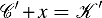 , where
  are their respective cromulent relabelings.
 , where
  . A sufficient extension is an extension that either: 1) closes an open gate; or 2) extends a full configuration such that the extension has at most one open gate. A configuration obtained by a series of sufficient extensions is a sufficient configuration if an (x,y)-, or an x/y-sequence can be applied to its cycles.
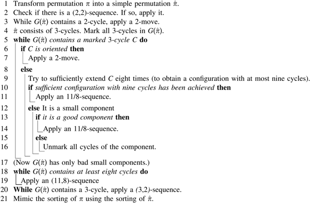


 (line 32). Later, if a well-behaved combination is found among the cycles in