A Fast Numerical Method for Max-Convolution and the Application to Efficient Max-Product Inference in Bayesian Networks

Abstract

Observations depending on sums of random variables are common throughout many fields; however, no efficient solution is currently known for performing max-product inference on these sums of general discrete distributions (max-product inference can be used to obtain maximum a posteriori estimates). The limiting step to max-product inference is the max-convolution problem (sometimes presented in log-transformed form and denoted as “infimal convolution,” “min-convolution,” or “convolution on the tropical semiring”), for which no O(k log(k)) method is currently known. Presented here is an O(k log(k)) numerical method for estimating the max-convolution of two nonnegative vectors (e.g., two probability mass functions), where k is the length of the larger vector. This numerical max-convolution method is then demonstrated by performing fast max-product inference on a convolution tree, a data structure for performing fast inference given information on the sum of n discrete random variables in O(nk log(nk)log(n)) steps (where each random variable has an arbitrary prior distribution on k contiguous possible states). The numerical max-convolution method can be applied to specialized classes of hidden Markov models to reduce the runtime of computing the Viterbi path from nk² to nk log(k), and has potential application to the all-pairs shortest paths problem.

1. Introduction

In many fields it is common to have access to information about sums of random variables and to desire information about those variables themselves. In mass spectrometry, when two (or more) analytes with similar mass-to-charge are measured, the intensity of the resulting peak is a function of the sum of abundances of those analytes (this problem occurs not only in the mass spectrometry of small molecules, but also in measuring isotope measurement in elemental and nuclear mass spectrometry). In transcriptomics, the abundance of a particular nonunique read (i.e., an RNA sequence that maps to multiple locations in the transcriptome or genome) provides information about the sum of the abundances of all transcripts that contain the read (each transcript weighted by how many copies of the read it carries). Proteomics has its own version of nonunique reads, shared peptides that can be found in multiple proteins [not only are shared peptides the principal source of difficulty in protein inference (Serang and Noble, 2012a, b; Serang et al. 2010), they are also responsible for the difficulty evaluating putatative sets of discovered proteins (Serang et al., 2012b, 2013)]. In population genetics, the prior knowledge about population structure can suggest an expected number of individuals with a particular genotype, which in turn yields probabilistic information about the individuals whose aggregate genotypes are expected to produce that sum [inference is particularly pronounced in polyploids, which increase the dimensionality of the problem (Serang et al., 2012a)].

In all of these fields, the information on sums of random variables presents a singular obstacle to computational biology. And regardless of how infrequently we as scientists directly discuss our current inability to effectively utilize information about sums of random variables, the perception of our limited ability to meet the challenge has become firmly entrenched in our collective unconscious; the silent agreement on our inability to turn the sausage grinder backward and convert the sausage (information about the sum of several random variables) back into the pigs (information about those random variables that contributed to the sum) is so well established that it not only defines the way we address these data (i.e., mass spectra peaks containing multiple analytes, counts of non unique reads, etc.), but it also causes us to discard data and even limit research directions we might otherwise consider. For instance, in mass spectrometry, substantial effort is invested in chromatography (Barnes, 1992; James and Martin, 1952) and other separation techniques (Pringle, et al., 2007), which aim to distinguish and separate analytes so that they will not be measured by the mass spectrometer simultaneously (thereby reducing the chances of analytes resulting in overlapping peaks); the task of decomposing this useful aggregate information from overlapping peaks back into information about its contributing parts is eschewed in favor of significant investments in instrumentation [e.g., more and more advanced separation technologies and higher-resolution mass spectrometers (Polacco et al., 2011)], and still it is common practice to discard shared isotope peaks and shared peptides even though they may comprise a large percent of the data and contain additional information (Dost et al., 2009; Serang et al., 2013). Likewise, in genomics and transcriptomics it is common to simply discard all data from nonunique reads (Lefrançois et al., 2009; Zentner et al., 2011). In burgeoning fields such as metagenomics, this loss of data—and subsequent loss of information—can be even more pronounced, for instance when all data that map to two or more species of interest are discarded. In some cases, recovering this lost information will be the key to making strong conclusions, such as distinguishing between two closely related species (or bacterial strains) in a metagenomic mixture.

1.1. Sum-product inference

Fast Fourier transform (FFT)-based convolution can be used to dramatically improve the efficiency of computing the sum-product addition of two discrete random variables. For three discrete random variables where M=L+R and where \documentclass{aastex}\usepackage{amsbsy}\usepackage{amsfonts}\usepackage{amssymb}\usepackage{bm}\usepackage{mathrsfs}\usepackage{pifont}\usepackage{stmaryrd}\usepackage{textcomp}\usepackage{portland, xspace}\usepackage{amsmath, amsxtra}\pagestyle{empty}\DeclareMathSizes{10}{9}{7}{6}\begin{document} $$L \in \{ 0 , 1 , \ldots k - 1 \} $$ \end{document} and \documentclass{aastex}\usepackage{amsbsy}\usepackage{amsfonts}\usepackage{amssymb}\usepackage{bm}\usepackage{mathrsfs}\usepackage{pifont}\usepackage{stmaryrd}\usepackage{textcomp}\usepackage{portland, xspace}\usepackage{amsmath, amsxtra}\pagestyle{empty}\DeclareMathSizes{10}{9}{7}{6}\begin{document} $$R \in \{ 0 , 1 , \ldots k - 1 \} $$ \end{document} , then the probability mass function (PMF) of M can be computed via the convolution of the PMFs of L and R, denoted pmf_L and pmf_R respectively. Note that it is sufficient to compute \documentclass{aastex}\usepackage{amsbsy}\usepackage{amsfonts}\usepackage{amssymb}\usepackage{bm}\usepackage{mathrsfs}\usepackage{pifont}\usepackage{stmaryrd}\usepackage{textcomp}\usepackage{portland, xspace}\usepackage{amsmath, amsxtra}\pagestyle{empty}\DeclareMathSizes{10}{9}{7}{6}\begin{document} $${ \rm pmf}_M^ \prime \propto { \rm pmf}_M$$ \end{document} , because the result will be scaled so that its sum is of unity ( \documentclass{aastex}\usepackage{amsbsy}\usepackage{amsfonts}\usepackage{amssymb}\usepackage{bm}\usepackage{mathrsfs}\usepackage{pifont}\usepackage{stmaryrd}\usepackage{textcomp}\usepackage{portland, xspace}\usepackage{amsmath, amsxtra}\pagestyle{empty}\DeclareMathSizes{10}{9}{7}{6}\begin{document} $$ { \rm pmf } _M = \frac { { \rm pmf } _M^ { \prime } } { \sum_m { \rm pmf } _M^ { \prime } [ m ] } $$ \end{document} ): \documentclass{aastex}\usepackage{amsbsy}\usepackage{amsfonts}\usepackage{amssymb}\usepackage{bm}\usepackage{mathrsfs}\usepackage{pifont}\usepackage{stmaryrd}\usepackage{textcomp}\usepackage{portland, xspace}\usepackage{amsmath, amsxtra}\pagestyle{empty}\DeclareMathSizes{10}{9}{7}{6}\begin{document} \begin{align*}{ \rm pmf}_M [ m ] & \propto \sum_ \ell \sum_r \Pr ( L = \ell ) { \rm Pr} ( R = r ) { \rm Pr} ( M = \ell + r ) \\ & \, = \sum_ \ell { \rm Pr} ( L = \ell ) { \rm Pr} ( R = m - \ell ) \\ & \, = { \rm pmf}_{L} * { \rm pmf}_{R}\end{align*} \end{document}

where * performs the convolution between the two k-length vectors storing each PMF.

Whereas naive convolution would compute pmf_M in O(k×k) steps, FFT exploits the bijection of this convolution to the product between two polynomials (where the vectors being convolved are the coefficients of the polynomials being multiplied and the coefficients of their product forms the vector result); this bijection enables the use of alternative forms for representing the polynomials (each order k − 1 polynomial can be represented through k unique points through which it passes), which in turn permits elegant divide and conquer algorithms such as the Cooley-Tukey FFT to compute fast convolution in k log(k) steps. 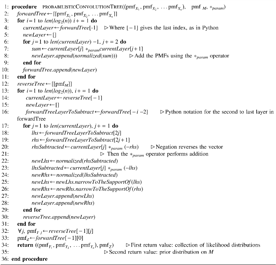Subtraction in the sum-product (i.e., computing L=M − R) scheme can be performed by first negating R′=−R (this is done by reversing the vector storing the PMF pmf_R′[r]=pmf_R[−r]), and then adding L=M+R′ as before via FFT convolution \documentclass{aastex}\usepackage{amsbsy}\usepackage{amsfonts}\usepackage{amssymb}\usepackage{bm}\usepackage{mathrsfs}\usepackage{pifont}\usepackage{stmaryrd}\usepackage{textcomp}\usepackage{portland, xspace}\usepackage{amsmath, amsxtra}\pagestyle{empty}\DeclareMathSizes{10}{9}{7}{6}\begin{document} $${ \rm pmf}_{L}^{ \prime} = { \rm pmf}_{M} * { \rm pmf}_{R^{ \prime}}$$ \end{document} . Also, the runtime constant on FFT convolution algorithms is generally very low, partly due to the nature of elegance of the algorithms and partly because implementations have been optimized heavily due to the ubiquity of convolution in signal processing.

The task of processing information about the sum of n discrete variables (each with k bins) to retrieve information on the individual variables can be performed naively in O(kⁿ) steps by simply enumerating the exponentially many possible outcomes; however, such brute-force techniques are wildly inefficient when either n or k become large. Fortunately, recent work proposes methods to decompose larger problems (e.g., into multiple sums and differences of pairs of discrete variables of the form M=L+R and L=M − R, very fast inference can be achieved). This has been derived for binary variables (k=2) in n log(n) log(n) (Tarlow et al., 2012), and was independently discovered for arbitrary discrete distributions (i.e., where k>2) and to multidimensional distributions (via matrix convolution, which can be decomposed into one-dimensional convolutions by the row-column algorithm) using the probabilistic convolution tree (Serang, 2014) (Algorithm 1). In the general case, distributions on all individual variables conditional on information about the sum can be computed in O(nk log(nk) log(n)) steps [whenever klog(k) fast convolution is available]:

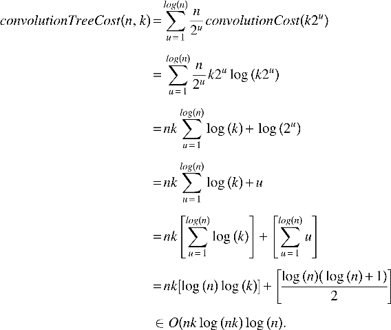
In practice, this can be significantly faster than the O(n²k²) steps required by dynamic programming when fast convolution is not available. For instance, when an observed transcript fragment could originate from n=256 species, and where the abundance of each species is discretized into k=1024 bins, then fast convolution makes inference more than 1800 times faster (the difference between one algorithm taking 1 sec and the other taking 30 min), and the disparity only grows for problems with larger values of n and k. It should be noted that these are only approximate runtimes calculated from the Big O form; in practice, it is fairly likely that methods based on fast convolution will be significantly faster, because of the method's inherent properties and the fact that very optimized implementations exist.

Algorithm 1.

The probabilistic convolution tree algorithm utilizes fast convolution (or fast max-convolution) to efficiently turn information on sums of variables back into information on the individual variables. The first parameter \documentclass{aastex}\usepackage{amsbsy}\usepackage{amsfonts}\usepackage{amssymb}\usepackage{bm}\usepackage{mathrsfs}\usepackage{pifont}\usepackage{stmaryrd}\usepackage{textcomp}\usepackage{portland, xspace}\usepackage{amsmath, amsxtra}\pagestyle{empty}\DeclareMathSizes{10}{9}{7}{6}\begin{document} $$ {\rm pmf_{x1}}, \ {\rm pmf_{y2}}, \ \cdots \ {\rm pmf_{yn}}$$ \end{document} is a collection of n multidimensional discrete distributions (with same dimension). In the case of univariate distributions, they are one-dimensional PMFs with k possible outcomes. The second parameter pmf_M is a multidimensional discrete distribution (with same dimension as X₁, X₂, …) where M = X₁ + X₂ + … + X_n. The third parameter is a convolution operator (e.g., either standard convolution or max-convolution). The algorithm returns a pair of values. The first is a collection of likelihood distributions given on the information from the sum M, \documentclass{aastex}\usepackage{amsbsy}\usepackage{amsfonts}\usepackage{amssymb}\usepackage{bm}\usepackage{mathrsfs}\usepackage{pifont}\usepackage{stmaryrd}\usepackage{textcomp}\usepackage{portland, xspace}\usepackage{amsmath, amsxtra}\pagestyle{empty}\DeclareMathSizes{10}{9}{7}{6}\begin{document} $$ (pmf_{y1}, pmf_{y2}, \cdots pmf_{yn} )$$ \end{document} . The second is the prior distribution of M after adding together all X₁ + X₂ + … X_n. When n is not an integer power of 2, dummy variables whose PMFs of length 1 (i.e., PMFs that are Kronecker deltas with 100% chance of having value 0) should be padded on until the next power of 2 is reached (this will allow construction of a full binary tree without changing the sum).

1.2. Max-product inference

Qualitatively, max-product inference is a close cousin to sum-product inference. Where sum-product inference considers each of the exponentially many joint events and allows each to contribute to the result (in hidden Markov models, this is analogous to the forward-backward algorithm), max-product inference allows only the highest-quality joint events to contribute (in hidden Markov models, this defines the Viterbi path). Both inference methods have complementary advantages and disadvantages: The advantage of sum-product inference is its democratized equal weighting of all joint events, the variety of which can provide a rich description of any high-probability joint events suggested by the data; however, this can also have disadvantages in that many low-quality joint events (i.e., those with low joint probability) may shape the result as much as a small number of high-quality results. Likewise, in sum-product inference, multiple mutually exclusive joint events can simultaneously contribute to the result, raising the potential to erroneously infer implausible conclusions, because both may be plausible before considering the other. It is because of these disadvantages in sum-product inference that max-product inference is widely used, because it forces the inferences to be jointly plausible (not simply individually, but as a whole), and because it drowns out noise from low-quality configurations that can diffuse and lower the certainty of conclusions in sum-product inference.

Specifically, efficient max-product inference on sums of random variables would be quite useful; in addition to the examples of shared peptides, nonunique reads, etc., found throughout computational biology (wherein we have information about the sum of variables, but want to draw conclusions about the variables themselves), more efficient max-product inference would make possible new inference algorithms on specialized classes of hidden Markov models (HMMs) where the transition probabilities from the state at index a to the state at index b depend on a function of either a+b or a−b or b−a. Such HMMs have applications in finance and time series analysis, where the k states at any layer are high-resolution discretizations of some quantity or price, and where the probability of a price moving up or down is influenced by the quantity up or down that it moved since the previous time point. In a general HMM with k states and n layers of those states, performing either sum-product (via the forward-backward algorithm) or max-product (via the Viterbi algorithm) inference requires O(nk²) steps; however, performing sum-product inference on the specialized class of HMMs mentioned above would require only O(nk log(k)) steps, because each layer can be processed as a two-node convolution tree. But finding the Viterbi path on such a model in O(nk log(k)) steps is not currently feasible, because doing so would require performing max-convolution (where the max of all valid pairings is chosen rather than the sum over all valid pairings) in O(k log(k)) steps.

However, despite the promise of max-product inference on sums of random variables, a fast practical solution that utilizes O(klog(k)) max-convolution (i.e., one with speed roughly comparable to FFT-based standard convolution) is not yet available for the general max-convolution problem. One special case, for use only when k=2 (Gupta et al., 2007; Tarlow et al., 2010), can solve the problem in nlog(n) time by sorting the n variables in descending order of probability \documentclass{aastex}\usepackage{amsbsy}\usepackage{amsfonts}\usepackage{amssymb}\usepackage{bm}\usepackage{mathrsfs}\usepackage{pifont}\usepackage{stmaryrd}\usepackage{textcomp}\usepackage{portland, xspace}\usepackage{amsmath, amsxtra}\pagestyle{empty}\DeclareMathSizes{10}{9}{7}{6}\begin{document} $${ \rm Pr} ( X_1 = 1 ) \geq { \rm Pr} ( X_2 = 1 ) \geq \cdots \geq { \rm Pr} ( X_n = 1 )$$ \end{document} and then exploiting the property that in any case where the number of “true” variables ∑_j X_j=m must prefer the first m variables in the sorted order. This method understandably fails when k>2 because there is no guarantee of an ordering that will satisfy all dimensions (when k=2, increasing the probability of Pr(X_j=1) has a useful effect of decreasing the probability of Pr(X_j=0) by the same amount in order to preserve the unitary value of the sum). When k>2, a similar idea to the sorting approach can be used, but not without approximation or some method for exploring or optimizing the exponential space of joint events (Serang et al., 2012a).

Adapting the probabilistic convolution tree algorithm from algorithm 1 (by simply replacing all uses of * with *_max when adding pairs of variables) achieves only an O(n²k²) runtime for max-product inference because additions and subtractions between individual pairs of random variables will require O(k²) time without a faster algorithm for max-convolution. It is tempting to try to derive an FFT equivalent to max-convolution, a subtle difference makes this challenging: Where standard convolution uses the operations (+, ×) on real-valued numbers (a “ring”), max-convolution employs (max, ×) [alternatively applying a log-transformation to the probabilities being convolved will negate them and thus change the problem to the equivalent (min, +) operations, called min-convolution, infimal convolution, or convolution on the “tropical semiring”]. Regardless of which form is used, the employment of the max (or min in the min-convolution case) downgrades the operation from a ring to a “semiring” because the max and min operations have no inverse. Thus, the max-product addition of two discrete random variables takes a different form, which is no longer bijective to polynomial multiplication: \documentclass{aastex}\usepackage{amsbsy}\usepackage{amsfonts}\usepackage{amssymb}\usepackage{bm}\usepackage{mathrsfs}\usepackage{pifont}\usepackage{stmaryrd}\usepackage{textcomp}\usepackage{portland, xspace}\usepackage{amsmath, amsxtra}\pagestyle{empty}\DeclareMathSizes{10}{9}{7}{6}\begin{document} \begin{align*}{ \rm pmf}_M [ m ] & \propto \max_ \ell \max_r { \rm Pr} ( L = \ell ) { \rm Pr} ( R = r ) { \rm Pr} ( M = \ell + r ) \\ & \,= \max_ \ell { \rm Pr} ( L = \ell ) { \rm Pr} ( R = m - \ell ) \\ & \,= { \rm pmf}_L *_{ \max} { \rm pmf}_R\end{align*} \end{document}

where *_max is the max-convolution operator. The loss of the bijective polynomial representation prevents the exploitation of the Lagrange form of polynomials, and thus there is no known klog(k) algorithm for performing max-convolution.

Excluding such highly specialized methods as the rank method of Babai Babai and Felzenszwalb (2009) [which achieves a runtime of \documentclass{aastex}\usepackage{amsbsy}\usepackage{amsfonts}\usepackage{amssymb}\usepackage{bm}\usepackage{mathrsfs}\usepackage{pifont}\usepackage{stmaryrd}\usepackage{textcomp}\usepackage{portland, xspace}\usepackage{amsmath, amsxtra}\pagestyle{empty}\DeclareMathSizes{10}{9}{7}{6}\begin{document} $$O ( k_1 \sqrt{k_2 \log ( k_2 ) } )$$ \end{document} time but only when the vector of length k₂ contains elements with value 0 or∞], the two most sophisticated max-convolution algorithms applicable to probabilistic inference are from Bussieck et al. (1994) and Bremner et al. (2006).

The method from Bussieck has a O(k²) runtime in the worst case, but under a certain distribution, values in the two vectors being convolved, the authors demonstrate an expected runtime of O(k log(k)) (Bussieck et al., 1994). The approach works by starting the result \documentclass{aastex}\usepackage{amsbsy}\usepackage{amsfonts}\usepackage{amssymb}\usepackage{bm}\usepackage{mathrsfs}\usepackage{pifont}\usepackage{stmaryrd}\usepackage{textcomp}\usepackage{portland, xspace}\usepackage{amsmath, amsxtra}\pagestyle{empty}\DeclareMathSizes{10}{9}{7}{6}\begin{document} $$\forall m , { \rm pmf}_M^{ \prime} [ m ] \gets - \infty$$ \end{document} and then proceeds by sorting the two vectors being convolved (L and R) in descending order. Their method then proceeds through both lists head-first to generate the first klog(k) sorted terms of ∀ℓ, r pmf_L[ℓ] pmf_R[r]. Each of these terms is used to update the appropriate index in the result vector \documentclass{aastex}\usepackage{amsbsy}\usepackage{amsfonts}\usepackage{amssymb}\usepackage{bm}\usepackage{mathrsfs}\usepackage{pifont}\usepackage{stmaryrd}\usepackage{textcomp}\usepackage{portland, xspace}\usepackage{amsmath, amsxtra}\pagestyle{empty}\DeclareMathSizes{10}{9}{7}{6}\begin{document} $${ \rm pmf}_M^{ \prime} [ \ell + r ] \gets \max ( { \rm pmf}_M^{ \prime} [ \ell + r ] , { \rm pmf}_L [ \ell ] { \rm pmf}_R [ r ] )$$ \end{document} . Thus far, the algorithm is ∈O(k log(k)), but there may be indices of \documentclass{aastex}\usepackage{amsbsy}\usepackage{amsfonts}\usepackage{amssymb}\usepackage{bm}\usepackage{mathrsfs}\usepackage{pifont}\usepackage{stmaryrd}\usepackage{textcomp}\usepackage{portland, xspace}\usepackage{amsmath, amsxtra}\pagestyle{empty}\DeclareMathSizes{10}{9}{7}{6}\begin{document} $${ \rm pmf}_M^{ \prime}$$ \end{document} that have not yet been set (they are still equal to −∞); each of these must be computed, and each such direct computation takes O(k) time [if there are Ω(k) such unset indices, then the overall runtime becomes O(k²)]. Despite the significant achievement posed by the construction of this algorithm, the authors suggest that the runtime constant is quite high due to the overhead of the sophisticated algorithms used to sort the largest k log(k) values while neither sorting nor even generating all k² values; they suggest that their result is of mostly theoretical import, and suggest using other methods in practice.

The method of Bremner et al. [which was subsequently extended by Williams (2014)] draws a relationship between min-convolution and the necklace alignment problem, wherein two collections of beads, each on its own circular string, are rotated to optimally align (Bremner et al., 2006). Their method is the most sophisticated in existence and consists of a highly complicated exploitation of similarity to the all-pairs shortest paths problem to achieve a method with a subquadratic worst-case runtime of \documentclass{aastex}\usepackage{amsbsy}\usepackage{amsfonts}\usepackage{amssymb}\usepackage{bm}\usepackage{mathrsfs}\usepackage{pifont}\usepackage{stmaryrd}\usepackage{textcomp}\usepackage{portland, xspace}\usepackage{amsmath, amsxtra}\pagestyle{empty}\DeclareMathSizes{10}{9}{7}{6}\begin{document} $$O ( k^2 \frac { { ( \log ( \log ( k ) ) ) } ^3 } { \log ( k ) \log ( k ) } )$$ \end{document} for each max-convolution [the runtime of the Bremner et al. method can also be improved using a more recent method for solving the all-pairs shortest paths problem, decreasing the runtime to \documentclass{aastex}\usepackage{amsbsy}\usepackage{amsfonts}\usepackage{amssymb}\usepackage{bm}\usepackage{mathrsfs}\usepackage{pifont}\usepackage{stmaryrd}\usepackage{textcomp}\usepackage{portland, xspace}\usepackage{amsmath, amsxtra}\pagestyle{empty}\DeclareMathSizes{10}{9}{7}{6}\begin{document} $$ \frac { k^2 } { 2^ { \Omega ( \sqrt { \log ( k ) } ) } } $$ \end{document} (Williams, 2014)]. Even if it were possble to be implemented with runtime constant as optimized as FFT, the cost of using a max-convolution tree to solve the previously mentioned metagenomic max-product inference problem on n=256 variables where each has k=1024 states would be over 166 times slower than the cost of solving an equally sized sum-product problem with FFT convolution (the number of steps required was calculated numerically to avoid computing a closed form of the computational cost).

Thus, even with significant mathematical sophistication of these two state-of-the-art methods, practically efficient max-product inference may be out of reach for even moderately sized problems.

2. A Numerical Method for Efficiently Estimating Max-Convolution

Here I will introduce a numerical method for estimating the max-convolution in k log(k) time, which can be applied easily using existing high-performance numerical software libraries. This is essentially performed by transforming both the inputs and outputs of the FFT to achieve p-norm convolution, which in turn is used as an approximation for max-convolution via the Chebyshev norm.

For a max-convolution between pmf_L and pmf_R \documentclass{aastex}\usepackage{amsbsy}\usepackage{amsfonts}\usepackage{amssymb}\usepackage{bm}\usepackage{mathrsfs}\usepackage{pifont}\usepackage{stmaryrd}\usepackage{textcomp}\usepackage{portland, xspace}\usepackage{amsmath, amsxtra}\pagestyle{empty}\DeclareMathSizes{10}{9}{7}{6}\begin{document} \begin{align*}{ \rm pmf}_M^{ \prime} [ m ] \,= \max_ \ell \,{ \rm pmf}_L [ \ell ] { \rm pmf}_R [ m - \ell ] ,\end{align*} \end{document}

at each m value, the shifted product's terms can be rewritten as a simple vector u^(m) where elements are defined by \documentclass{aastex}\usepackage{amsbsy}\usepackage{amsfonts}\usepackage{amssymb}\usepackage{bm}\usepackage{mathrsfs}\usepackage{pifont}\usepackage{stmaryrd}\usepackage{textcomp}\usepackage{portland, xspace}\usepackage{amsmath, amsxtra}\pagestyle{empty}\DeclareMathSizes{10}{9}{7}{6}\begin{document} \begin{align*}u^{ ( m ) } [ \ell ] = { \rm pmf}_L [ \ell ] { \rm pmf}_R [ m - \ell ].\end{align*} \end{document}

Furthermore, because PMFs consist of nonnegative real values (or machine-precision representations), then this can be rewritten using the Chebyshev norm, which computes the maximum absolute value in the vector u^(m). Because u^(m) comes from the product of PMF terms, it is also nonnegative and thus absolute values can be ignored in both the computation and the result: \documentclass{aastex}\usepackage{amsbsy}\usepackage{amsfonts}\usepackage{amssymb}\usepackage{bm}\usepackage{mathrsfs}\usepackage{pifont}\usepackage{stmaryrd}\usepackage{textcomp}\usepackage{portland, xspace}\usepackage{amsmath, amsxtra}\pagestyle{empty}\DeclareMathSizes{10}{9}{7}{6}\begin{document} \begin{align*} { \rm pmf } _M^ { \prime } [ m ] & = \max_ \ell u^ { ( m ) } [ \ell ] \\ \mid { \rm pmf } _M^ { \prime } [ m ] \mid & = \lim_ { p \rightarrow \infty } \parallel u^ { ( m ) } \parallel_p \\ \mid { \rm pmf } _M^ { \prime } [ m ] \mid & = \lim_ { p \rightarrow \infty } { \left( \sum_ \ell \mid { u^ { ( m ) } [ \ell ] } \mid^p \right) } ^ \frac { 1 } { p } \\ { \rm pmf } _M^ { \prime } [ m ] & = \lim_ { p \rightarrow \infty } { \left( \sum_ \ell { u^ { m ) } [ \ell ] } ^p \right) } ^ \frac { 1 } { p } . \end{align*} \end{document}

And then each element of u^(m)[ℓ] can be expanded back into its original factors: \documentclass{aastex}\usepackage{amsbsy}\usepackage{amsfonts}\usepackage{amssymb}\usepackage{bm}\usepackage{mathrsfs}\usepackage{pifont}\usepackage{stmaryrd}\usepackage{textcomp}\usepackage{portland, xspace}\usepackage{amsmath, amsxtra}\pagestyle{empty}\DeclareMathSizes{10}{9}{7}{6}\begin{document} \begin{align*} { \rm pmf } _M^ { \prime } [ m ] = \lim_ { p \rightarrow \infty } { \left( \sum_ \ell { { \rm pmf } _L [ \ell ] } ^p { { \rm pmf } _R [ m - \ell ] } ^p \right) } ^ \frac { 1 } { p } .\end{align*} \end{document}

At this point, a sufficiently large value p* is used in place of the limit p→∞ : \documentclass{aastex}\usepackage{amsbsy}\usepackage{amsfonts}\usepackage{amssymb}\usepackage{bm}\usepackage{mathrsfs}\usepackage{pifont}\usepackage{stmaryrd}\usepackage{textcomp}\usepackage{portland, xspace}\usepackage{amsmath, amsxtra}\pagestyle{empty}\DeclareMathSizes{10}{9}{7}{6}\begin{document} \begin{align*} { \rm pmf } _M^ { \prime } [ m ] \approx { \left( \sum_ \ell { { \rm pmf } _L [ \ell ] } ^ { p^* } { { \rm pmf } _R [ m - \ell ] } ^ { p^* } \right) } ^ \frac { 1 } { p^* } .\end{align*} \end{document}

At this point, it can be observed that every time elements of the PMFs pmf_L[ℓ] and pmf_R[m − ℓ] appear, they are raised to the p* power; thus, it is possible to change variables and let \documentclass{aastex}\usepackage{amsbsy}\usepackage{amsfonts}\usepackage{amssymb}\usepackage{bm}\usepackage{mathrsfs}\usepackage{pifont}\usepackage{stmaryrd}\usepackage{textcomp}\usepackage{portland, xspace}\usepackage{amsmath, amsxtra}\pagestyle{empty}\DeclareMathSizes{10}{9}{7}{6}\begin{document} \begin{align*} \forall \ell \ v_L [ \ell ] & = {{ \rm pmf}_L [ \ell ] }^{p^*} \\ \forall r \ v_R [ r ] & = {{ \rm pmf}_R [ r ] }^{p^*} , \end{align*} \end{document}

yielding \documentclass{aastex}\usepackage{amsbsy}\usepackage{amsfonts}\usepackage{amssymb}\usepackage{bm}\usepackage{mathrsfs}\usepackage{pifont}\usepackage{stmaryrd}\usepackage{textcomp}\usepackage{portland, xspace}\usepackage{amsmath, amsxtra}\pagestyle{empty}\DeclareMathSizes{10}{9}{7}{6}\begin{document} \begin{align*} { \rm pmf } _M^ { \prime } [ m ] \approx { \left( \sum_ \ell v_L [ \ell ] v_R [ m - \ell ] \right) } ^ \frac { 1 } { p^* } .\end{align*} \end{document}

A similar strategy can be made for \documentclass{aastex}\usepackage{amsbsy}\usepackage{amsfonts}\usepackage{amssymb}\usepackage{bm}\usepackage{mathrsfs}\usepackage{pifont}\usepackage{stmaryrd}\usepackage{textcomp}\usepackage{portland, xspace}\usepackage{amsmath, amsxtra}\pagestyle{empty}\DeclareMathSizes{10}{9}{7}{6}\begin{document} $${ \rm pmf}_M^{ \prime}$$ \end{document} ; it is possible to introduce another vector v_M such that every element \documentclass{aastex}\usepackage{amsbsy}\usepackage{amsfonts}\usepackage{amssymb}\usepackage{bm}\usepackage{mathrsfs}\usepackage{pifont}\usepackage{stmaryrd}\usepackage{textcomp}\usepackage{portland, xspace}\usepackage{amsmath, amsxtra}\pagestyle{empty}\DeclareMathSizes{10}{9}{7}{6}\begin{document} $${ \rm pmf}_M^{ \prime} [ m ]$$ \end{document} is the result of \documentclass{aastex}\usepackage{amsbsy}\usepackage{amsfonts}\usepackage{amssymb}\usepackage{bm}\usepackage{mathrsfs}\usepackage{pifont}\usepackage{stmaryrd}\usepackage{textcomp}\usepackage{portland, xspace}\usepackage{amsmath, amsxtra}\pagestyle{empty}\DeclareMathSizes{10}{9}{7}{6}\begin{document} \begin{align*} { \rm pmf } _M^ { \prime } [ m ] & \approx { v_M [ m ] } ^ { \frac { 1 } { p^* } } \\ v_M [ m ] & \,= \sum_ \ell v_L [ \ell ] v_R [ m - \ell ] \end{align*} \end{document}

And thus it becomes clear that v_M is the result of standard convolution (not a max-convolution) between v_L and v_R. This suggests a numerical algorithm that can make use of existing FFT convolution libraries to compute v_M=v_L * v_R in O(k log(k)) steps (Algorithm 2).

Algorithm 2.

Numerical max-convolution (initial version), a numerical method to estimate the max-convolution of two PMFs or nonnegative vectors. The parameters are two PMFs, pmf_L and pmf_R (by definition nonnegative), and the numerical value p* used for computation. The return value is a numerical estimate of the max-convolution pmf_L *_max pmf_R.

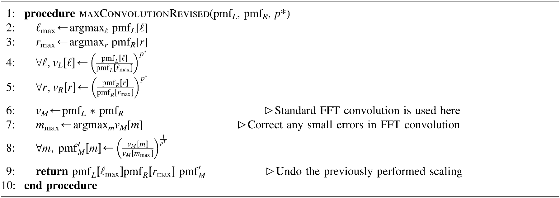
2.1. Reducing underflow

The main caveat for numerical methods is often the loss of precision due to underflow when raising small probabilities to the power p* (in this case, no overflow occurs because the inputs are probabilities); such losses may not be undone later when raising to the \documentclass{aastex}\usepackage{amsbsy}\usepackage{amsfonts}\usepackage{amssymb}\usepackage{bm}\usepackage{mathrsfs}\usepackage{pifont}\usepackage{stmaryrd}\usepackage{textcomp}\usepackage{portland, xspace}\usepackage{amsmath, amsxtra}\pagestyle{empty}\DeclareMathSizes{10}{9}{7}{6}\begin{document} $$ { \frac {1} {p^{*}}}$$ \end{document} power. One way to limit unnecessary loss of precision is to recognize that it is possible to scale \documentclass{aastex}\usepackage{amsbsy}\usepackage{amsfonts}\usepackage{amssymb}\usepackage{bm}\usepackage{mathrsfs}\usepackage{pifont}\usepackage{stmaryrd}\usepackage{textcomp}\usepackage{portland, xspace}\usepackage{amsmath, amsxtra}\pagestyle{empty}\DeclareMathSizes{10}{9}{7}{6}\begin{document} $${ \rm pmf}_M^{ \prime}$$ \end{document} arbitrarily during computation (and then scaling it back afterward). For this reason it can be beneficial to scale a vector by dividing by its maximum element before raising it to the p* or \documentclass{aastex}\usepackage{amsbsy}\usepackage{amsfonts}\usepackage{amssymb}\usepackage{bm}\usepackage{mathrsfs}\usepackage{pifont}\usepackage{stmaryrd}\usepackage{textcomp}\usepackage{portland, xspace}\usepackage{amsmath, amsxtra}\pagestyle{empty}\DeclareMathSizes{10}{9}{7}{6}\begin{document} $$ { \frac {1} {p^{*}}}$$ \end{document} power; this will start the dominant elements close to 1, and thus allow them to lose little information to underflow. Using this strategy yields a slightly modified algorithm (Algorithm 3).

Algorithm 3.

Numerical max-convolution (normalized version), a numerical method to estimate the max-convolution of two PMFs or nonnegative vectors (revised to reduce underflow). The parameters are two PMFs pmf_L and pmf_R (by definition nonnegative) and the numerical value p* used for computation. The return value is a numerical estimate of the max-convolution pmf_L *_max pmf_R.

Note that, like standard implementations of fast convolution *, in implementing the fast *_max operator it is possible to automatically choose between a naive implementation or the fast numerical implementation depending on the size of the problem; on very small problems (e.g., k=8), the naive operation will have less overhead and can be a bit faster [the specific threshold can be chosen roughly by comparing the expected running time from the fast numerical method O(k′log(k′))—where k′ is double the next integer power of two and the log is base two—to the O(k²) naive method]; this can reduce numerical error further.

3. Results

I briefly compare the speed and accuracy of the fast numerical max-convolution method as compared to naive max-convolution. Both methods are implemented in the Python programming language using floating point math and the numpy package (the fast numerical max-convolution method is implemented from Algorithm 3.

3.1. Practical efficiency of fast numerical max-convolution

The speed of naive max-convolution is compared to the fast numerical estimate. For each k ∈{32, 64, 128, 256, 512, 1024, 2048, 4096, 8192}, random pairs of vectors with uniform elements [i.e., each element is drawn from uniform(0, 1)]. The result of the max-convolution \documentclass{aastex}\usepackage{amsbsy}\usepackage{amsfonts}\usepackage{amssymb}\usepackage{bm}\usepackage{mathrsfs}\usepackage{pifont}\usepackage{stmaryrd}\usepackage{textcomp}\usepackage{portland, xspace}\usepackage{amsmath, amsxtra}\pagestyle{empty}\DeclareMathSizes{10}{9}{7}{6}\begin{document} $${ \rm pmf}_{L}^{ \prime} = { \rm pmf}_{M} * { \rm pmf}_{R^{ \prime}}$$ \end{document} is computed via O(k²) naive max-convolution and the fast numerical method. Figure 1 demonstrates a substantial speedup in practice.

FIG. 1.

Runtime comparison between naive and fast numerical convolution. Note the increasing gap between the two curves indicates a nonlinear speedup due to the log scaling of both axes (because the runtime of the fast numerical method is dominated by Fast Fourier transform (FFT) calculation).

3.2. Accuracy of fast numerical max-convolution compared to naive max-convolution

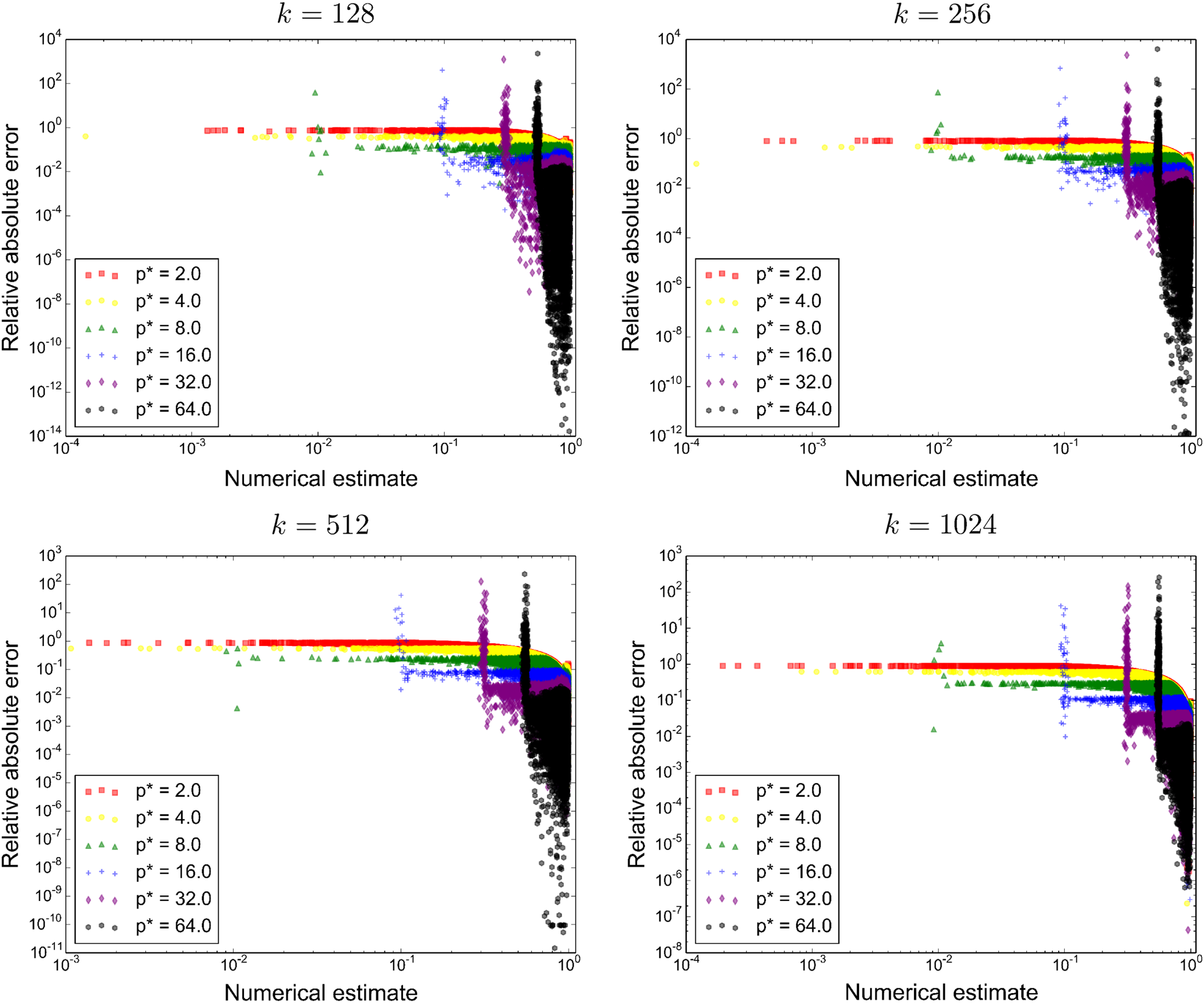
A cursory empirical test of the numerical stability as a result of p* and the vector length k was performed. In Figure 2, the numerical stability was demonstrated on 64 random pairs of vectors for each length k ∈128, 256, 512, 1024. For all p* ∈{2, 4, 8, 16, 32, 64}, and the relative absolute error of each element in the result of the max-convolution is computed \documentclass{aastex}\usepackage{amsbsy}\usepackage{amsfonts}\usepackage{amssymb}\usepackage{bm}\usepackage{mathrsfs}\usepackage{pifont}\usepackage{stmaryrd}\usepackage{textcomp}\usepackage{portland, xspace}\usepackage{amsmath, amsxtra}\pagestyle{empty}\DeclareMathSizes{10}{9}{7}{6}\begin{document} $$\mid \frac { numerical [ m ] - exact [ m ] } { exact [ m ] } \mid$$ \end{document} , where numerical[m] and exact[m] refer to the value at index m of the numerical and naive results respectively. Figure 2 demonstrates the relationship between p*, k, the relative absolute error, and the magnitude of the exact result.

FIG. 2.

The influence of the parameter p* on max-convolution accuracy. For each k ∈{128, 256, 512, 1024}, 64 replicate max-convolutions are performed to compare the relative error of the fast numerical method compared to the naive method. This is performed for different values of p*; lower values of p* perform well when the exact result is close to zero, and higher values of p* perform better otherwise, and this relationship is invariant of k when the data are scaled in the manner presented (they are scaled so that the largest element has value 1).

Algorithm 4.

Numerical max-convolution (piecewise version), a numerical method to estimate the max-convolution of two PMFs or nonnegative vectors (further revised to strategically choose p*). The parameters are two PMFs, pmf_L and pmf_R both with k outcomes (and both by definition nonnegative). The return value is a numerical estimate of the max-convolution pmf_L *_max pmf_R. This algorithm calls the revised method maxConvolutionRevised from Algorithm 3. Note that the values of \documentclass{aastex}\usepackage{amsbsy}\usepackage{amsfonts}\usepackage{amssymb}\usepackage{bm}\usepackage{mathrsfs}\usepackage{pifont}\usepackage{stmaryrd}\usepackage{textcomp}\usepackage{portland, xspace}\usepackage{amsmath, amsxtra}\pagestyle{empty}\DeclareMathSizes{10}{9}{7}{6}\begin{document} $$ P^{*}_{lower} , P^{*}_{higher} $$ \end{document} , and Τ specified here may be chosen to optimize performance on a specific application.

Qualitatively, optimizing the numerical performance involves satisfying competing ideals: when p* is large, the problem solved converges to the max-convolution inference, but underflow becomes significant. When p* is too small, nonmaximal terms contribute to the result (more similar to a standard convolution).

Although more sophisticated numerical analysis would almost certainly yield larger improvements to the method, a simple improvement is exploited: Generally the relative error is fairly low, but only becomes high in these experiments when the exact value at that index is close to zero (this is intuitive from the formula for relative absolute error). Since underflow allowed to propagate through the FFT is the only numerical consideration (overflow before the FFT does not occur because the values are normalized to the maximum), then it follows that a result that is not close to zero at some index is a high-quality estimate when p* is substantially large (if it suffered from too much underflow, then it would approach zero quickly). Therefore, when using a high value of p*, indices where the numerical solution is close to zero indicate the potential for numerical error and suggest that a smaller value of p* could be used for those indices. This yields a further improvement where a more accurate result can be constructed from two calls of Algorithm 3; this improved method is shown in Algorithm 4, and runs in roughly twice as many steps as Algorithm 3 [still ∈O(klog(k))]. Note that this piecewise method could be trivially extended to use more than two values of p*, increasing accuracy at the expense of additional runtime (although, assuming the results using the different values of p* are computed in decreasing order, then the routine could potentially terminate once the result has been estimated at all indices with adequate numeric stability).

3.3. Using fast numerical convolution to solve a probabilistic subset sum problem

Lastly, a three-way piecewise implementation of max-convolution similar to the one shown in Algorithm 4 but using p* ∈{4, 32, 64} (the Python code of this three-way piecewise method is given in the accompanying Python demonstration code) is used to solve a simulated probabilistic generalization of the the subset sum problem [note that even the deterministic subset sum problem is very similar to the definition of the knapsack problem from Karp's 21 NP-complete problems and is itself NP-complete (Karp, 1972)]. In this problem, n=32 people go shopping and each person j in \documentclass{aastex}\usepackage{amsbsy}\usepackage{amsfonts}\usepackage{amssymb}\usepackage{bm}\usepackage{mathrsfs}\usepackage{pifont}\usepackage{stmaryrd}\usepackage{textcomp}\usepackage{portland, xspace}\usepackage{amsmath, amsxtra}\pagestyle{empty}\DeclareMathSizes{10}{9}{7}{6}\begin{document} $$\{ 1 , 2 , \ldots n \} $$ \end{document} buys exactly one of two items (the price of the item they do purchase is \documentclass{aastex}\usepackage{amsbsy}\usepackage{amsfonts}\usepackage{amssymb}\usepackage{bm}\usepackage{mathrsfs}\usepackage{pifont}\usepackage{stmaryrd}\usepackage{textcomp}\usepackage{portland, xspace}\usepackage{amsmath, amsxtra}\pagestyle{empty}\DeclareMathSizes{10}{9}{7}{6}\begin{document} $$\mu_j^{ ( true ) }$$ \end{document} , and the price of the item they do not purchase is \documentclass{aastex}\usepackage{amsbsy}\usepackage{amsfonts}\usepackage{amssymb}\usepackage{bm}\usepackage{mathrsfs}\usepackage{pifont}\usepackage{stmaryrd}\usepackage{textcomp}\usepackage{portland, xspace}\usepackage{amsmath, amsxtra}\pagestyle{empty}\DeclareMathSizes{10}{9}{7}{6}\begin{document} $$\mu_j^{ ( false ) }$$ \end{document} ), where the costs of both items for each person j are unknown to us. Then, given fuzzy knowledge about the costs of these items, with all prices discretized into k=256 bins (i.e., ∀j, pmf_Xj[ℓ] where \documentclass{aastex}\usepackage{amsbsy}\usepackage{amsfonts}\usepackage{amssymb}\usepackage{bm}\usepackage{mathrsfs}\usepackage{pifont}\usepackage{stmaryrd}\usepackage{textcomp}\usepackage{portland, xspace}\usepackage{amsmath, amsxtra}\pagestyle{empty}\DeclareMathSizes{10}{9}{7}{6}\begin{document} $$\ell \in \{ 0 , 1 , \ldots k - 1 \} $$ \end{document} ) and given fuzzy knowledge about the total amount spent (pmf_M, where M=∑_j X_j), we try to infer the amount spent by each person (i.e., for each person j, estimating \documentclass{aastex}\usepackage{amsbsy}\usepackage{amsfonts}\usepackage{amssymb}\usepackage{bm}\usepackage{mathrsfs}\usepackage{pifont}\usepackage{stmaryrd}\usepackage{textcomp}\usepackage{portland, xspace}\usepackage{amsmath, amsxtra}\pagestyle{empty}\DeclareMathSizes{10}{9}{7}{6}\begin{document} $$\mu_j^{ ( true ) }$$ \end{document} ).

Data are generated as follows: At each variable \documentclass{aastex}\usepackage{amsbsy}\usepackage{amsfonts}\usepackage{amssymb}\usepackage{bm}\usepackage{mathrsfs}\usepackage{pifont}\usepackage{stmaryrd}\usepackage{textcomp}\usepackage{portland, xspace}\usepackage{amsmath, amsxtra}\pagestyle{empty}\DeclareMathSizes{10}{9}{7}{6}\begin{document} $$X_j , j \in \{ 1 , 2 , \ldots n \} $$ \end{document} , two means are randomly sampled \documentclass{aastex}\usepackage{amsbsy}\usepackage{amsfonts}\usepackage{amssymb}\usepackage{bm}\usepackage{mathrsfs}\usepackage{pifont}\usepackage{stmaryrd}\usepackage{textcomp}\usepackage{portland, xspace}\usepackage{amsmath, amsxtra}\pagestyle{empty}\DeclareMathSizes{10}{9}{7}{6}\begin{document} $$\mu_j^{ ( true ) } , \mu_j^{ ( false ) } \sim uniform ( 0 , k - 1 )$$ \end{document} , and a discretized Gaussian PMF is centered about each mean [the standard deviations of the Gaussians are each sampled \documentclass{aastex}\usepackage{amsbsy}\usepackage{amsfonts}\usepackage{amssymb}\usepackage{bm}\usepackage{mathrsfs}\usepackage{pifont}\usepackage{stmaryrd}\usepackage{textcomp}\usepackage{portland, xspace}\usepackage{amsmath, amsxtra}\pagestyle{empty}\DeclareMathSizes{10}{9}{7}{6}\begin{document} $$\sigma_j^ { ( true ) } , \sigma_j^ { ( false ) } \sim uniform ( 0 , \frac { k } { 10 } )$$ \end{document} ]. A vector proportional to the PMF pmf_Xj[ℓ] is computed using the sum of these Gaussians with a vector of uniform noise α⁽ⁱⁿ⁾[ℓ]∼uniform(0, 0.0001). The likelihood distribution on the sum M=∑_j X_j is generated by adding a Gaussian with mean ∑_jμ_j^(true) and variance 0.005×(nk−(n − 1)) (i.e., 0.005×the possible number of outcomes for M), plus point-wise samples of uniform noise α^(out)[ℓ]∼uniform(0, 0.0001).

On each problem instance, likelihoods for all inputs ( \documentclass{aastex}\usepackage{amsbsy}\usepackage{amsfonts}\usepackage{amssymb}\usepackage{bm}\usepackage{mathrsfs}\usepackage{pifont}\usepackage{stmaryrd}\usepackage{textcomp}\usepackage{portland, xspace}\usepackage{amsmath, amsxtra}\pagestyle{empty}\DeclareMathSizes{10}{9}{7}{6}\begin{document} $${ \rm pmf}_{Y_1} , { \rm pmf}_{Y_2} , \ldots { \rm pmf}_{Y_n}$$ \end{document} ) are computed twice, once using naive max-convolution and once using the numerical method. Note that even though these values of n and k do not appear particularly large, the full max-convolution tree that they produce will compute several max-convolutions on the order of O(k) and a few on the order of O(n×k), which in this case can be 32×256=8192. For this reason, computing the likelihood curve with the naive result requires 159 sec, while the fast numerical approach takes 0.935 sec to compute a highly similar result.

A single likelihood distribution \documentclass{aastex}\usepackage{amsbsy}\usepackage{amsfonts}\usepackage{amssymb}\usepackage{bm}\usepackage{mathrsfs}\usepackage{pifont}\usepackage{stmaryrd}\usepackage{textcomp}\usepackage{portland, xspace}\usepackage{amsmath, amsxtra}\pagestyle{empty}\DeclareMathSizes{10}{9}{7}{6}\begin{document} $${ \rm pmf}_{Y_j}$$ \end{document} for one particular \documentclass{aastex}\usepackage{amsbsy}\usepackage{amsfonts}\usepackage{amssymb}\usepackage{bm}\usepackage{mathrsfs}\usepackage{pifont}\usepackage{stmaryrd}\usepackage{textcomp}\usepackage{portland, xspace}\usepackage{amsmath, amsxtra}\pagestyle{empty}\DeclareMathSizes{10}{9}{7}{6}\begin{document} $$j \in \{ 1 , 2 , \ldots n \} $$ \end{document} , which was computed using the naive method; the fast numerical method is plotted in Figure 3. This figure also demonstrates the utility of max-product inference by also showing the result from sum-product inference, which is much less informative (and does not have a mode close to the correct answer).

FIG. 3.

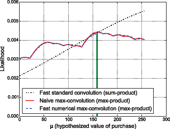
Using fast numerical max-convolution for max-product inference. A single likelihood distribution for an arbitrary \documentclass{aastex}\usepackage{amsbsy}\usepackage{amsfonts}\usepackage{amssymb}\usepackage{bm}\usepackage{mathrsfs}\usepackage{pifont}\usepackage{stmaryrd}\usepackage{textcomp}\usepackage{portland, xspace}\usepackage{amsmath, amsxtra}\pagestyle{empty}\DeclareMathSizes{10}{9}{7}{6}\begin{document} $$j \in \{ 1 , 2 , \ldots , n \} $$ \end{document} from a probabilistic generalization of the subset-sum problem with n=32 and k=256 is shown. This distribution is computed via a probabilistic max-convolution tree (the problem is solved twice, once with naive max-convolution and once via fast numerical max-convolution). The true mode value \documentclass{aastex}\usepackage{amsbsy}\usepackage{amsfonts}\usepackage{amssymb}\usepackage{bm}\usepackage{mathrsfs}\usepackage{pifont}\usepackage{stmaryrd}\usepackage{textcomp}\usepackage{portland, xspace}\usepackage{amsmath, amsxtra}\pagestyle{empty}\DeclareMathSizes{10}{9}{7}{6}\begin{document} $$\mu_j^{ ( true ) }$$ \end{document} for that j is indicated by the bar beneath the largest mode. To compare the results of different types of inference, the sum-product result from the convolution tree (using the standard convolution operator) is also plotted; note that sum-product inference produces a less discriminative likelihood curve because many possible joint events have diffused into it.

4. Discussion

Although its ethos may ultimately limit the utility of this method to numerical settings where small errors are tolerable [as opposed to the to more general theoretical articles previously mentioned (Bussieck et al., 1994; Bremner et al. 2006)], the numerical method proposed here gives a simple and very fast estimate of the max-convolution result, which could allow use of numerical max-convolution (or max-product inference on the sums and differences between discrete distributions) in settings where it is currently far too computationally expensive. The largest caveat to the method is the inaccuracy that can occur due to numerical bottlenecks (e.g., underflow); however, for many problems (e.g., practical applications of the max-product inference problem in Fig. 3), the numerical method is sufficient to perform high-quality inference, but in a dramatically faster time.

Furthermore, the connection between the max-convolution problem and the all-pairs shortest path problem from graph theory (Bremner et al. 2006) means that the fast numerical method can be used to compute fast numerical approximations to that important computer science problem. Such fast numerical estimates could complement theoretical solutions to that problem.

A more in-depth theoretical analysis of the algorithm's error would likely yield multiple opportunities to modify the algorithm in order to decrease error. For example, one possible improvement could be performed by using log-transformed real values: in log-transformed space, raising to the power p* would be equivalent to scaling by p* and would not produce significant underflow. Furthermore, the operations required by FFT convolution could be performed in log-space by translating the ring (+, ×) on real values to its equivalent ring (log₊, log_×)=(log₊, +) on log-transformed values, where the operation log₊(x, y) is performed by dividing out the greater of the two arguments x (w.l.o.g.) and then computing \documentclass{aastex}\usepackage{amsbsy}\usepackage{amsfonts}\usepackage{amssymb}\usepackage{bm}\usepackage{mathrsfs}\usepackage{pifont}\usepackage{stmaryrd}\usepackage{textcomp}\usepackage{portland, xspace}\usepackage{amsmath, amsxtra}\pagestyle{empty}\DeclareMathSizes{10}{9}{7}{6}\begin{document} $$\log ( 1 + \frac { y } { x } ) =\log ( 1 + z )$$ \end{document} via Taylor series; performing the Cooley-Tukey FFT on log-transformed values (or possibly using a different FFT algorithm that is particularly well suited for log-transformed values) could represent one route for improving the accuracy.

In a similar vein, more sophisticated techniques for locally choosing among a small number of values for p* (compared to a simple piecewise function on two possible values of p*). For instance, under roughly uniform distributions of values in the two vectors being max-convolved, the values closest to zero (and thus having higher chance of having high relative absolute error) will occur more commonly at the first and last indices of the numerical estimate (because those indices take the maximum over smaller collections of elements, and are thus more likely to be smaller values). Similar attention could be put toward scaling the vectors prior to taking elements to the p* (compared to the current procedure of dividing by the maximum element value) may minimize the underflow on a large number of points with large values. A most exciting possibility would be that having an accurate estimate of the max-convolution result somehow could be used to compute a more accurate result (e.g., using approximate results from different p* and exploiting the property ‖·‖_p≥‖·‖_p+δ when p≥1 and δ > 0). Such directions of future research could possibly solving the max-convolution iteratively over a bounded or constant number of subproblems where each subproblem requires O(klog(k)), by first computing initial estimates of the max-convolution result with the numerical method presented here, and then using those initial estimates to parameterize a subsequent call to the numerical method in a manner reminiscent of the QR algorithm for eigendecomposition (Francis, 1961, 1962). From Algorithm 4, it seems highly likely that there will be more ways by which an initial result can be used to obtain a higher-accuracy result.

Furthermore, even pursuing methods for obtaining very high accuracy with large values of p* may not always be of substantial interest. Indeed, even if no improvement to accuracy is ever presented, the design and parameterization of machine learning methods (including graphical models) has traditionally been empirically driven, and the use of exact max-product inference is hardly sacrosanct in every application (as opposed to inference somewhere between sum-product and max-product). From this perspective, rather than choosing p* as a static constant value p*=1 (i.e., performing sum-product inference) or p*→∞ (i.e., performing max-product inference), p* could be viewed as a hyperparameter that is used to position inference on a continuum somewhere between all joint events contributing equally to the end result (sum-product) and only the best joint event contributing (max-product), and intermediate values of p* would establish a preference for the top few joint events. In this sense, the value chosen for p* could be driven by the data, and the problem of p-norm convolution (where a finite p is desired, rather than max-convolution where p→∞ ) can already be solved with very high accuracy by the proposed numerical method for any moderate choice of p*.

Acknowledgments

Thanks to Mattias Franberg and Ryan Emerson for the helpful comments.

Footnotes

Author Disclosure Statement

No competing financial interests exist.

References

Babai

, and Felzenszwalb

P.F.

2009. Computing rank-convolutions with a mask. ACM Trans. Algorithms., 6, 20.

Barnes

1992. High Performance Liquid Chromatography, volume 33. John Wiley & Sons, New York.

Bremner

, Chan

T.M.

, Demaine

E.D.

, et al. 2006. Necklaces, convolutions, and X+Y, 160–171. In Algorithms–ESA 2006. Springer, New York.

Bussieck

, Hassler

, Woeginger

G.J.

, et al. 1994. Fast algorithms for the maximum convolution problem. Oper. Res. Lett., 15, 133–141.

Dost

, Bandeira

, Li

, et al. 2009. Shared peptides in mass spectrometry based proteomics, 356–371. In Batzoglou

, ed. Proceedings of the Thirteenth Annual International Conference on Computational Molecular Biology, volume 13.

Francis

J.G.F.

1961. The QR transformation a unitary analogue to the LR transformationpart 1. Comput. J., 4, 265–271.

Francis

J.G.F.

1962. The QR transformationpart 2. Comput. J., 4, 332–345.

Gupta

, Diwan

A.A.

, and Sarawagi

2007. Efficient inference with cardinalitybased clique potentials, 329–336. In Proceedings of the 24th International Conference on Machine Learning.

James

A.T.

, and Martin

A.J.P.

1952. Gas-liquid partition chromatography: the separation and micro-estimation of volatile fatty acids from formic acid to dodecanoic acid. Biochem. J., 50, 679.

10.

Karp

R.M.

1972. Reducibility among combinatorial problems, 85–103. In Miller

R.E.

, and Thatcher

J.W.

, eds. Complexity of Computer Computations. Plenum Press, New York.

11.

Lefrançois

, Euskirchen

G.M.

, Auerbach

R.K.

, et al. 2009. Efficient yeast chip-seq using multiplex short-read dna sequencing. BMC Genomics., 10, 37.

12.

Polacco

B.J.

, Purvine

S.O.

, Zink

E.M.

, et al. 2011. Discovering mercury protein modifications in whole proteomes using natural isotope distributions observed in liquid chromatography-tandem mass spectrometry. Mol. Cell. Proteomics., 10, M110-004853.

13.

Pringle

S.D.

, Giles

, Wildgoose

J.L.

, et al. 2007. An investigation of the mobility separation of some peptide and protein ions using a new hybrid quadrupole/travelling wave ims/oa-tof instrument. Int. J. Mass Spectrom., 261, 1–12.

14.

Serang

2014. The probabilistic convolution tree: efficient exact bayesian inference for faster LC-MS/MS protein inference. PloS One., 9, e91507.

15.

Serang

, and Noble

W.S.

2012a. A review of statistical methods for protein identification using tandem mass spectrometry. Stat. Its Interface., 5, 3–20.

16.

Serang

, and Noble

W.S.

2012b. Faster mass spectrometry-based protein inference: junction trees are more efficient than sampling and marginalization by enumeration. IEEE/ACM Trans. Comput. Biol. Bioinform., 9, 809–817.

17.

Serang

, MacCoss

M.J.

, and Noble

W.S.

2010. Efficient marginalization to compute protein posterior probabilities from shotgun mass spectrometry data. J. Proteome Res., 9, 5346–5357.

18.

Serang

, Mollinari

, and Garcia

2012a. Efficient exact maximum a posteriori computation for Bayesian SNP genotyping in polyploids. PLoS ONE. 7, e30906.

19.

Serang

, Moruz

, Hoopmann

M.R.

, and Käll

2012b. Recognizing uncertainty increases robustness and reproducibility of mass spectrometry-based protein inferences. J. Proteome Res., 11, 5586–5591.

20.

Serang

, Paulo

, Steen

, et al. 2013. A non-parametric cutout index for robust evaluation of identified proteins. Mol. Cell. Proteomics., 12, 807–812.

21.

Tarlow

, Givoni

I.E.

, and Zemel

R.S.

2010. HOP-MAP: efficient message passing with high order potentials. International Conference on Artificial Intelligence and Statistics, pp. 812–819.

22.

Tarlow

, Swersky

, Zemel

R.S.

, et al. 2012. Fast exact inference for recursive cardinality models. arXiv preprint arXiv:1210.4899.

23.

Williams

2014. Faster all-pairs shortest paths via circuit complexity, 664–673. In Proceedings of the 46th Annual ACM Symposium on Theory of Computing. STOC ’14. ACM.

24.

Zentner

G.E.

, Saiakhova

, Manaenkov

, et al. 2011. Integrative genomic analysis of human ribosomal DNA. Nucleic Acids Res. 39, 4949–4960.