An Efficient Algorithm for the Contig Ordering Problem under Algebraic Rearrangement Distance

Abstract

Assembling a genome from short reads currently obtained by next-generation sequencing techniques often results in a collection of contigs, whose relative position and orientation along the genome being sequenced are unknown. Given two sets of contigs, the contig ordering problem is to order and orient the contigs in each set such that the genome rearrangement distance between the resulting sets of ordered and oriented contigs is minimized. In this article, we utilize the permutation groups in algebra to propose a near-linear time algorithm for solving the contig ordering problem under algebraic rearrangement distance, where the algebraic rearrangement distance between two sets of ordered and oriented contigs is the minimum weight of applicable rearrangement operations required to transform one set into the other.

1. Introduction

The next-generation sequencing (NGS) techniques have greatly advanced during the past decade (Shendure and Ji, 2008; Metzker, 2010; van Dijk et al., 2014), allowing an increasing number of genomes to be sequenced rapidly in a decreasing cost. However, assembling a genome from short reads currently obtained by the NGS techniques often results in a draft genome with a collection of contigs, whose relative position and orientation along the genome being sequenced are unknown. A scaffolding process is then applied to a draft genome for determining the ordering and orientation of its contigs (Bentley, 2006; Pop, 2009). The accuracy of the scaffolding process is important and helpful to obtain a complete genome of an organism in the subsequent finishing process, which usually utilizes the so-called primer walking technique to closing the gaps between ordered and oriented contigs.

Resequencing is one of the most commonly used approaches in the scaffolding process (Bentley, 2006). The resequencing methods usually require a complete genome of a related organism to serve as a reference. They map the contigs of a draft genome onto a reference genome and then try to infer the ordering and orientation of the contigs according to their positions on the reference genome. Currently, several algorithms based on the resequencing approach have been proposed (van Hijum et al., 2005; Gaul and Blanchette, 2006; Richter et al., 2007; Assefa et al., 2009; Rissman et al., 2009; Muñoz et al., 2010; Husemann and Stoye, 2010; Galardini et al., 2011; Dias et al., 2012; Li et al., 2013; Lu et al., 2014). In fact, all these algorithms can be classified into two categories: alignment-based ones and rearrangement-based ones. The alignment-based algorithms (van Hijum et al., 2005; Richter et al., 2007; Assefa et al., 2009; Rissman et al., 2009; Husemann and Stoye, 2010; Galardini et al., 2011) align contigs or contig ends of a draft genome against a reference sequence, and then ordered and oriented the contigs according to the positions of their matches in the reference. As to the rearrangement-based algorithms (Gaul and Blanchette, 2006; Muñoz et al., 2010; Dias et al., 2012; Li et al., 2013; Lu et al., 2014), they attempt to order and orient the contigs of a draft genome in a way such that the orders of conserved genes (or genetic markers) between the ordered and oriented draft genome and the reference genome are as similar as possible.

When addressing the scaffolding of contigs in a draft genome using the rearrangement-based approach, we formulated the one-sided contig (or block) ordering problem (Li et al., 2013) as follows. Given a draft genome and a reference of complete genome, the one-sided contig ordering problem is to order and orient the contigs of the draft genome such that the genome rearrangement distance between the resulting draft genome and the reference genome is minimized. The sets of ordered and oriented contigs in the resulting draft genome are then called scaffolds. In our previous study (Li et al., 2013), we used the chromosomal algebraic model to represent the draft and reference genomes and utilized the permutation groups in algebra to design an \documentclass{aastex}\usepackage{amsbsy}\usepackage{amsfonts}\usepackage{amssymb}\usepackage{bm}\usepackage{mathrsfs}\usepackage{pifont}\usepackage{stmaryrd}\usepackage{textcomp}\usepackage{portland, xspace}\usepackage{amsmath, amsxtra}\pagestyle{empty}\DeclareMathSizes{10}{9}{7}{6}\begin{document} $${ \cal O}$$ \end{document} (δn) time algorithm for solving the one-sided contig ordering problem, when the genome rearrangement distance is measured by reversals and block-interchanges with the weight ratio 1:2, where n is the number of genes and δ is the number of used reversals and block-interchanges. Note that the above time complexity includes the cost for computing the scenario of the needed reversals and block-interchanges. On the other hand, if the reference is allowed to be a draft genome (but not necessarily a complete genome), then the problem mentioned above is called the (two-sided) contig ordering problem, which was introduced by Gaul and Blanchette (Gaul and Blanchette, 2006) and defined as follows. Given two sets of contigs as two draft genomes, the contig ordering problem is to order and orient the contigs of both the input draft genomes such that the genome rearrangement distance between the resulting scaffolds of the two draft genomes is minimized. In Gaul and Blanchette (2006), they propose a linear-time algorithm to solve the contig ordering problem if the problem is further simplified to maximize the number of cycles in the breakpoint graph between the ordered and oriented draft and reference genomes.

Recently, Feijão and Meidanis (2013) introduced a new way to model genomes, called the adjacency algebraic model, which can be considered as a combination of the algebraic model we used to solve the one-sided contig ordering problem and the adjacency graph proposed by Bergeron et al. (2006) to simplify the formalization of genomes and the computation of rearrangement distance. The genome rearrangement distance defined under the adjacency algebraic model is called algebraic (rearrangement) distance, which is the minimum weight of applicable rearrangement operations required to transform one of the genomes being compared into the other. Basically, the algebraic rearrangement distance is very similar to, but not the same as, the so-called double-cut-and-join (DCJ) distance (Yancopoulos et al., 2005). The main reason for their difference is due to the different weights assigned to some rearrangement operations. The operations of linear fusion/fission and circularization/linearization have weight ½ in the adjacency algebraic model, while they have weight 1 in the DCJ model. For all other rearrangement operations, such as reversals, transpositions, and block-interchanges, they have the same weight in both models. In this study, we utilize the permutation groups in algebra to propose a near-linear time algorithm for solving the contig ordering problem under the algebraic rearrangement distance, which aims at ordering and orienting the contigs of two input draft genomes such that the algebraic rearrangement distance between the resulting scaffolds of the draft genomes is minimized. Compared with the algorithm proposed by Gaul and Blanchette (2006) based on the breakpoint graphs, our algorithm can be implemented efficiently using simple operations in the permutation groups and the union and find operations of the disjoint-set data structure.

The rest of this article is organized as follows. Some basic concepts and properties of permutation groups in algebra, as well as the algebraic models for representing genomes, are introduced in section 2. In section 3, we present a near-linear time algorithm based on the techniques of the permutation groups to solve the contig ordering problem under the algebraic rearrangement distance. Finally, we make a brief conclusion in section 4.

2. Preliminaries

2.1. Basic concepts of permutation groups

Given a set E={1, 2,…,n}, a permutation α is a one-to-one function from E into itself. Basically, a permutation can be represented by a production of cycles in which each element is followed by its image. For example, α=(1, 3, 2)(4)(5, 6) is a permutation of E={1, 2,…, 6}, meaning that α(1)=3,α(3)=2,α(2)=1, α(4)=4, α(5)=6, and α(6)=5. The elements in a cycle of a permutation can be arranged in any cyclic order. Hence, the cycle (1, 2, 3) of α in the above example can also be rewritten as (2, 3, 1) or (3, 1, 2). If the cycles in a permutation are all disjoint (i.e., no common element in any two cycles), then the product of these cycles is called the cycle decomposition of the permutation. A cycle with k elements is called a k-cycle. Since a 1-cycle represents a fixed element in the permutation, it is usually not written explicitly. For instance, α=(1, 3, 2)(4)(5, 6) can be simply written as α=(1, 3, 2)(5, 6). If the cycles in a permutation are all 1-cycles, then this permutation is called an identity permutation and denoted by 1.

Suppose that α and β are two permutations of E. Then their product αβ, also called composition, defines a permutation of E satisfying αβ(x)=α(β(x)) for all x ∈E. If both α and β are disjoint cycles, then αβ=βα. If αβ=1, then α is called the inverse of β, denoted by β⁻¹, and vice versa. For a permutation that is expressed as a product of disjoint cycles, then its inverse can be obtained by just reversing the order of the elements in each cycle. For example, the inverse of (1, 3, 2)(5, 6) is (2, 3, 1)(6, 5). The conjugation of β by α, denoted by α · β, is defined to be the permutation αβα⁻¹. It can be verified that if β(x)=y, then α · β(α(x))=α(y). This means that α · β can be obtained from β by just changing each element x with α(x). That is, if β=(b₁,b₂,…,b_k), then α · β=(α(b₁),α(b₂),…,α(b_k)).

In fact, every permutation can be expressed into a product of 2-cycles, not necessarily disjoint, in which 1-cycles are still written implicitly. Given a permutation α of E, its norm, denoted by ∥α∥, is defined to be the minimum number, say k, such that α can be expressed as a product of k 2-cycles. In the cycle decomposition of α, let nc(α) denote the number of its disjoint cycles, notably including the 1-cycles not written explicitly. In Huang and Lu (2010), it has been proved that ∥α∥=|E|−nc(α).

Given two permutations α and β of E, α is said to divide β, denoted by α|β, if ∥βα⁻¹∥=∥β∥−∥α∥. The property described below in Lemma 2.1 is useful to determine whether or not a cycle (a₁,a₂,…,a_k) divides the permutation α.

Lemma 2.1 (Huang and Lu, 2010) Let a₁,a₂,…,a_k be in E, and α be a permutation of E in the form of cycle decomposition. Then a₁,a₂,…,a_k appear in a cycle of α in the ordering of a₁,a₂,…,a_k if and only if (a₁,a₂,…,a_k)|α.

Let α=(a₁,a₂) be a 2-cycle and β be any permutation of E. Suppose that α|β. Then a₁ and a₂ are in the same cycle in β according to Lemma 2.1. As a result, this cycle will be broken into two smaller ones in the composition of αβ (or βα). For example, if α=(1, 3) and β=(1, 2, 3, 4), then αβ=(1, 2)(3, 4) and βα=(4, 1)(2, 3). In other words, α functions on β as a split operation. On the other hand, suppose that α ∤β. Then a₁ and a₂ are in two different cycles in β according to Lemma 2.1. Moreover, these two cycles will be joined into a bigger one in αβ (or βα). For example, if α=(1, 3) and β=(1, 2)(3, 4), then αβ=(1, 2, 3, 4) and βα=(2, 1, 4, 3). Hence, α functions on β as a join operation.

2.2. Genes, chromosomes, and genomes

A gene is an oriented sequence of DNA that starts with a tail and ends with a head. Basically, a gene has two orientations (i.e., forward and backward) and is usually represented by a signed integer, with the sign indicating its orientation, in the studies of genome rearrangements (Lu et al., 2006; Huang and Lu, 2010). A chromosome is then represented by a sequence of ordered genes and a genome by a set of chromosomes. Note that a chromosome can be either linear or circular. In this study, a linear chromosome is further represented as a sequence of ordered genes enclosed in brackets and a circular chromosome as a sequence of ordered genes enclosed in angle brackets. For example, {[1,−2, 3],〈−4, 5,−6〉} denotes a genome consisting of a linear chromosome [1,−2, 3] and a circular chromosome 〈−4, 5,−6〉.

2.3. Representing genomes using a set of adjacencies

For a gene x, its tail and head are also called extremities and denoted by x_t and x_h, respectively. An adjacency is a set of two extremities to denote a connection between two adjacent genes on a chromosome. A telomere is an extremity not adjacent to any other extremity on a chromosome and represented by a singleton set. Actually, a genome for a given set \documentclass{aastex}\usepackage{amsbsy}\usepackage{amsfonts}\usepackage{amssymb}\usepackage{bm}\usepackage{mathrsfs}\usepackage{pifont}\usepackage{stmaryrd}\usepackage{textcomp}\usepackage{portland, xspace}\usepackage{amsmath, amsxtra}\pagestyle{empty}\DeclareMathSizes{10}{9}{7}{6}\begin{document} $${ \cal G}$$ \end{document} of genes can be further represented by a set of adjacencies and telomeres such that each extremity appears in exactly one adjacency or telomere. For example, the genome {[1,−2, 3],〈−4, 5,−6〉} can be represented by {{1_t}, {1_h, 2_h}, {2_t, 3_t}, {3_h}, {4_t, 5_t}, {5_h, 6_h}, {6_t, 4_h}} as illustrated in Figure 1. Usually, the telomeres in a genome can be omitted, since they can be uniquely determined from the gene set \documentclass{aastex}\usepackage{amsbsy}\usepackage{amsfonts}\usepackage{amssymb}\usepackage{bm}\usepackage{mathrsfs}\usepackage{pifont}\usepackage{stmaryrd}\usepackage{textcomp}\usepackage{portland, xspace}\usepackage{amsmath, amsxtra}\pagestyle{empty}\DeclareMathSizes{10}{9}{7}{6}\begin{document} $${ \cal G}$$ \end{document} . Therefore, the genome shown in Figure 1 can be further simplified as {{1_h, 2_h}, {2_t, 3_t}, {4_t, 5_t}, {5_h, 6_h}, {6_t, 4_h}}. Two adjacencies are said to be conflicting if they share at least one extremity in common. Basically, a genome (without gene duplication) can be represented by a set of mutually nonconflicting adjacencies. On the other hand, a set of mutually nonconflicting adjacencies can be considered as a valid genome.

FIG. 1.

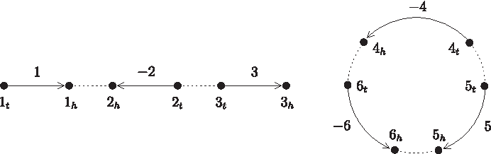
Graph representation of a genome {[1,−2, 3]〈−4, 5,−6〉}, where vertices represent extremities, directed solid edges represent genes, and undirected dotted edges represent adjacencies.

2.4. Representing genomes using algebraic models

Let n be the number of genes and E_n={−1, 1,−2, 2,…,−n,n} be the set of all genes in forward and backward orientations. The set E_n is used to model genomes with n genes as permutations. Let Γ=(−1, 1)(−2, 2)…(−n,n) denote the permutation of E_n that maps each gene into its reverse complement or, equivalently, inverts the sign (orientation) of a gene. It can be easily verified that Γ²=1 and hence Γ⁻¹=Γ. Currently, there are two algebraic models that can be used to represent genomes. The first one is called chromosomal algebraic model, which was first introduced by Meidanis and Dias (2000) to represent circular chromosomes only and then expanded by Feijão and Meidanis (2013) to represent both circular and linear chromosomes. In the chromosomal algebraic model, circular and linear chromosomes are represented in two different ways. For a circular chromosome α=〈a₁,a₂,…,a_k〉, it is modeled as a permutation α_chr that is the product of two disjoint cycles π and Γ · π⁻¹, that is, α_chr=π(Γ · π⁻¹), where π=(a₁,a₂,…,a_k), representing a strand of α, and Γ · π⁻¹ is the reverse complement of π. In this representation, both strands of α are expressed by different cycles in a permutation. For example, a circular chromosome α=〈−4, 5,−6〉 is represented by a permutation α_chr=(−4, 5, −6)(6, −5, 4) in the chromosomal algebraic model (Fig. 2b). On the other hand, for a linear chromosome β=[b₁,b₂,…,b_k], it is modeled by a permutation with a single cycle β_chr=(b₁,b₂,…,b_k, Γb_k, Γb_k₋₁…, Γb₁) in the chromosomal algebraic representation. In such a representation, both strands of a linear chromosome are together expressed by using a single cycle. For example, a linear chromosome β=[1,−2, 3] is represented by a permutation β_chr=(1,−2, 3,−3, 2,−1) in the chromosomal algebraic model (Fig. 2a). Note that in the above representation, an extremity u is a telomere of linear chromosome β if u=β_chrΓ(u).

FIG. 2.

In the chromosomal algebraic model, (a) a linear chromosome β=[1,−2, 3] is represented as a permutation with a cycle β_chr=(1,−2, 3,−3, 2,−1) and (b) a circular chromosome α=〈−4, 5, −6〉 as a permutation with two disjoint cycles α_chr=(−4, 5,−6)(6,−5, 4).

The second algebraic model is called adjacency algebraic model, which was introduced by Feijão and Meidanis (2013) to model both circular and linear chromosomes in a uniform way. In the adjacency algebraic model, the tail and head of a gene x are further denoted by +x and −x, respectively (i.e., x_t = +x and x_h=−x). Moreover, a genome is represented by a permutation that is a product of 2-cycles and 1-cycles, with each 2-cycle corresponding to an adjacency and each 1-cycle corresponding to a telomere in the genome, where the 1-cycles in this permutation can be omitted. For instance, a genome π={[1,−2, 3]〈−4, 5,−6〉} is represented by a permutation π_adj=(−1,−2)(2, 3)(4, 5)(−5,−6)(6,−4) in the adjacency algebraic model.

Feijão and Meidanis (2013) proposed an interesting property as follows to show the relationship between chromosomal and adjacency algebraic models. Multiplying a genome on the right by Γ switches the representation of a genome between chromosomal and adjacency algebraic representations. More formally, let π_chr and π_adj respectively denote the chromosomal and adjacency algebraic representations of a given genome π. Then π_chrΓ=π_adj and π_adjΓ=π_chr. For example, suppose that π={[1, −2, 3]〈−4, 5,−6〉}. Then π_chr=(1, −2, 3, −3, 2, 1)(−4, 5, −6)(6, −5, 4) and π_adj=(−1, −2)(2, 3)(4, 5)(−5, −6)(6,−4). It can be verified that π_chrΓ=π_adj and π_adjΓ=π_chr. If ρ is a rearrangement event that can transform π_chr into another genome σ_chr (i.e., ρπ_chr=σ_chr), then ρπ_chrΓ=σ_chrΓ and hence ρπ_adj=σ_adj. It indicates that the rearrangement event acting on a genome can be represented by the same permutation in both the chromosomal and adjacency algebraic models. In addition, \documentclass{aastex}\usepackage{amsbsy}\usepackage{amsfonts}\usepackage{amssymb}\usepackage{bm}\usepackage{mathrsfs}\usepackage{pifont}\usepackage{stmaryrd}\usepackage{textcomp}\usepackage{portland, xspace}\usepackage{amsmath, amsxtra}\pagestyle{empty}\DeclareMathSizes{10}{9}{7}{6}\begin{document} $$ \sigma_{ \rm chr} \pi_{ \rm chr}^{ - 1} = \sigma_{ \rm adj} \Gamma ( \pi_{ \rm adj} \Gamma ) ^{ - 1} = \sigma_{ \rm adj} \Gamma \Gamma^{ - 1} \pi_{ \rm adj}^{ - 1} = \sigma_{ \rm adj} \pi_{ \rm adj}^{ - 1} $$ \end{document} . In other words, the permutation σπ⁻¹ remains the same in both the chromosomal and adjacency algebraic models.

2.5. Algebraic rearrangement problem

As mentioned previously, any set of mutually nonconflicting adjacencies is a valid genome. Therefore, any permutation with a product of disjoint 2-cycles can represent a valid genome in the adjacency algebraic model. Let π and σ be two permutations representing two genomes in the adjacency algebraic representation. A rearrangement operation applicable to a genome π is defined as a permutation ρ that can be applied to π such that ρπ is a valid genome. Moreover, the weight of an applicable rearrangement operation ρ is defined as \documentclass{aastex}\usepackage{amsbsy}\usepackage{amsfonts}\usepackage{amssymb}\usepackage{bm}\usepackage{mathrsfs}\usepackage{pifont}\usepackage{stmaryrd}\usepackage{textcomp}\usepackage{portland, xspace}\usepackage{amsmath, amsxtra}\pagestyle{empty}\DeclareMathSizes{10}{9}{7}{6}\begin{document} $$ \frac { \parallel \rho \parallel } { 2 } $$ \end{document} . The so-called algebraic rearrangement problem, introduced by Feijão and Meidanis (2013), is to find a sequence of applicable rearrangement operations ρ₁,ρ₂,…,ρ_k that can transform π into σ such that the weight of this sequence \documentclass{aastex}\usepackage{amsbsy}\usepackage{amsfonts}\usepackage{amssymb}\usepackage{bm}\usepackage{mathrsfs}\usepackage{pifont}\usepackage{stmaryrd}\usepackage{textcomp}\usepackage{portland, xspace}\usepackage{amsmath, amsxtra}\pagestyle{empty}\DeclareMathSizes{10}{9}{7}{6}\begin{document} $$\sum \nolimits_ { i = 1 } ^k \frac { \parallel \rho_i \parallel } { 2 } $$ \end{document} is minimized. The weight of such a sequence is then called algebraic (rearrangement) distance and denoted by d(π,σ).

Lemma 2.2 (Feijão and Meidanis, 2013) Given two genomes π and σ, the algebraic rearrangement distance between them is \documentclass{aastex}\usepackage{amsbsy}\usepackage{amsfonts}\usepackage{amssymb}\usepackage{bm}\usepackage{mathrsfs}\usepackage{pifont}\usepackage{stmaryrd}\usepackage{textcomp}\usepackage{portland, xspace}\usepackage{amsmath, amsxtra}\pagestyle{empty}\DeclareMathSizes{10}{9}{7}{6}\begin{document} $$d ( \pi , \sigma ) = \frac { \parallel \sigma \pi^ { - 1 } \parallel } { 2 } $$ \end{document} .

According to Lemma 2.2, the norm of σπ⁻¹ is equal to 2d(π,σ). A permutation ρ is said to be a sorting operation from π to σ if ρπ is a valid genome and \documentclass{aastex}\usepackage{amsbsy}\usepackage{amsfonts}\usepackage{amssymb}\usepackage{bm}\usepackage{mathrsfs}\usepackage{pifont}\usepackage{stmaryrd}\usepackage{textcomp}\usepackage{portland, xspace}\usepackage{amsmath, amsxtra}\pagestyle{empty}\DeclareMathSizes{10}{9}{7}{6}\begin{document} $$d ( \rho \pi , \sigma ) = d ( \pi , \sigma ) - \frac { \parallel \rho \parallel } { 2 } $$ \end{document} .

Lemma 2.3 (Feijão and Meidanis, 2013) Given two genomes π and σ, if ρ is a sorting operation from π to σ, then ρ divides σπ⁻¹, that is, ρ|σπ⁻¹.

By Lemma 2.3, a sorting operation from π to σ is an applicable rearrangement operation on π such that ρ|σπ⁻¹. Feijão and Meidanis (2013) have shown that one can always find a sequence of sorting operations ρ₁,ρ₂,…,ρ_k such that ρ_kρ_k₋₁…ρ₁π=σ and \documentclass{aastex}\usepackage{amsbsy}\usepackage{amsfonts}\usepackage{amssymb}\usepackage{bm}\usepackage{mathrsfs}\usepackage{pifont}\usepackage{stmaryrd}\usepackage{textcomp}\usepackage{portland, xspace}\usepackage{amsmath, amsxtra}\pagestyle{empty}\DeclareMathSizes{10}{9}{7}{6}\begin{document} $$\sum \nolimits_ { i = 1 } ^ { k } \frac { \parallel \rho_i \parallel } { 2 } = d ( \pi , \sigma )$$ \end{document} . As described in Theorem 2.1 below, they have also demonstrated that the algebraic rearrangement distance between π and σ can be determined by a formula that is totally based on the numbers of cycles and paths in the adjacency graph between π and σ. The adjacent graph between π and σ, denoted by AG(π,σ), is defined as a graph in which the vertices are the adjacencies and telomeres of π and σ and for each vertex u in π and each vertex v in σ, there is an edge between u and v if u and v have an extremity in common (see Fig. 3 for an example). Clearly, as illustrated in Figure 3, an adjacency graph is composed exclusively of paths and cycles, since the degree of each vertex is less than or equal to two.

FIG. 3.

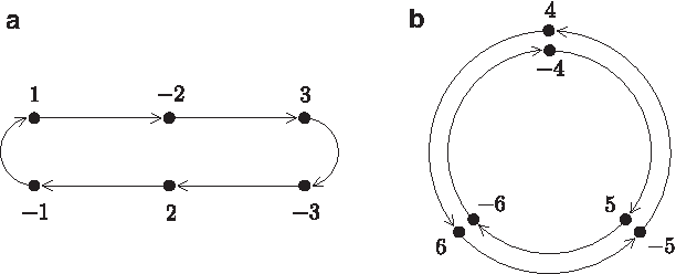
The adjacency graph of two genomes π={[1, 4], [3, 2], [−5, 6], [7, 8]} and σ={[1, 2, 3], [4, 5], [6, 7, 8]}, where the vertex corresponding to an adjacency {x,y} is simply labeled as xy and the vertex corresponding to a telomere {z} as z.

Theorem 2.1 (Feijão and Meidanis, 2013) The algebraic rearrangement distance between two genomes π and σ is \documentclass{aastex}\usepackage{amsbsy}\usepackage{amsfonts}\usepackage{amssymb}\usepackage{bm}\usepackage{mathrsfs}\usepackage{pifont}\usepackage{stmaryrd}\usepackage{textcomp}\usepackage{portland, xspace}\usepackage{amsmath, amsxtra}\pagestyle{empty}\DeclareMathSizes{10}{9}{7}{6}\begin{document} $$d ( \pi , \sigma ) = N - C - \frac { P } { 2 } $$ \end{document} , where N is the number of genes, C is the number of cycles, and P is the number of paths in the adjacency graph AG(π,σ).

3. Algorithm

Note that the genomes considered below are unichromosomal. Given two draft genomes π and σ, with each draft genome represented by a set of contigs, our task in this study is to order and orient the contigs in these two draft genomes such that the algebraic rearrangement distance between the resulting scaffolds of π and σ is minimized. It can be observed that when all the contigs in π and σ are ordered and oriented completely, the adjacency graph obtained from the resulting π and σ has only two paths, if π and σ are two linear chromosomes. This is because only four vertices, which correspond to telomeres in the resulting scaffolds of π and σ, in the adjacency graph have degree one and the others corresponding to adjacencies have degree two. On the other hand, if π and σ are circular chromosomes, then the adjacency graph between the ordered and oriented π and σ has no paths, since all the vertices correspond to adjacencies and thus have degree two. In other words, after completely ordering and orienting all the contigs in both π and σ, the number of paths in their resulting adjacency graph is fixed (either two or zero), meaning that the algebraic rearrangement distance between the ordered and oriented π and σ totally depends on the number of cycles in their adjacency graph according to Theorem 2.1. Therefore, the contig ordering problem under the algebraic rearrangement distance is equivalent to ordering and orienting the contigs in π and σ such that the number of cycles in the adjacency graph between the resulting π and σ is maximized.

Let π_chr and σ_chr denote two draft genomes π and σ respectively in the chromosomal algebraic representation. Note that for a permutation α and an element x, we rewrite α(x) as αx for simplicity, if the context is clear. In fact, ordering and orienting two contigs in π_chr or σ_chr can be considered as a fusion of these two contigs (i.e., joining them into a bigger one). Basically, contigs are linear chromosomal fragments. Then according to the algebraic theory (Feijão and Meidanis, 2013), a fusion of two contigs c₁ and c₂ in π_chr can be modeled by applying a 2-cycle ρ=(Γu,v) to π_chr, as illustrated in Figure 4, where Γu and v are telomeres in c₁ and c₂, respectively. Let π_adj and σ_adj denote π and σ respectively in the adjacency algebraic representation, that is, π_adj=π_chrΓ and σ_adj=σ_chrΓ. In this representation, Γu and v are fixed elements in π_adj and hence applying ρ to π_adj will join telomeres Γu and v into a 2-cycle (Γu,v). Moreover, such an action will correspondingly lead to telomere vertices Γu and v in the adjacency graph AG(π,σ) being joined as an adjacency vertex {Γu,v}. In AG(π,σ), a telomere vertex must be an end of a path. Suppose that Γu and v are ends in two paths p₁ and p₂, respectively, in AG(π,σ). Then applying ρ to π_adj will also lead to the paths p₁ and p₂ in AG(π,σ) being joined together as a longer one. However, if p₁=p₂ (i.e., Γu and v are the ends of the same path), then applying ρ to π_adj will cause the path p₁ in AG(π,σ) being circularized as a cycle.

FIG. 4.

(a) Two contigs c₁ and c₂ of a draft genome π_chr in the chromosomal algebraic representation, where dashed edges denote paths of consecutive solid edges. (b) Contigs c₁ and c₂ are joined together in ρπ_chr, where ρ=(Γu,v) and Γu and v are telomeres of c₁ and c₂, respectively.

Recall that our goal in this study is to find the orderings and orientations of the contigs in two draft genomes π and σ such that the number of cycles in the adjacency graph between the resulting scaffolds of π and σ is maximized. As mentioned above, ordering and orienting two contigs in π or σ is equivalent to finding a fusion to join these two contigs. Moreover, applying a fusion on π or σ to join two of its contigs results in either merging two paths in AG(π,σ) into a longer one or closing a path as a cycle. Hence, the best case occurs when each of all the paths in AG(π,σ) is closed as a cycle by a fusion. Actually, not every path in AG(π,σ) can be closed by a fusion. The criteria for closing a path p in AG(π,σ) by a fusion are as follows: (1) the length of p is even, and (2) both the ends of p correspond to the telomeres in two different contigs in π or σ. If p has odd length, then one end of p corresponds to a telomere of one contig c₁ in π and the other end corresponds to a telomere of another contig c₂ in σ. In this case, c₁ and c₂ are in different genomes and hence they cannot be joined together by a fusion. If the length of p is even and both ends of p are the telomeres of the same contig in π or σ, then closing p will create a circular contig, which is not allowed in the process of ordering and orienting contigs. According to the discussion above, we call a fusion as a good fusion if it can close a path in AG(π,σ) when applying to π or σ, and we also call the path being closed as a good path.

In fact, for a nongood path p₁ of even length in AG(π,σ), we can join it with any other path p₂ by a nongood fusion at any time in the process of ordering and orienting contigs, which does not affect the optimal solution. The reason is described as follows. Basically, there are three cases for p₂: (1) p₂ is a good path, (2) p₂ is an odd path, and (3) p₂ is an even but nongood path. If p₂ is a good (respectively, odd and nongood even) path, then the join of p₁ and p₂ through a nongood fusion is still a good (respectively, odd and nongood even) path. It implies that no matter what the path p₂ is, the numbers of good and odd paths remain the same after joining p₁ with p₂, but the number of nongood even paths is decreased by one. Actually, we can imagine that after joining with any other path p₂, the nongood even path p₁ will disappear without changing anything except extending the length of p₂. It suggests that the number of cycles created by joining contigs is not related to the number of nongood even paths. Therefore, it does not matter when we join a nongood even path with another path by using a nongood fusion in the whole process of ordering and orienting contigs.

For a good path p₁ in AG(π,σ), it can be joined with any nongood even path, as discussed above. However, it is better to close p₁ as a cycle rather than to join it with a good or odd path p₂ as a longer path, when we want to find an optimal way to order and orient the contigs in π and σ. The reason is as follows. Suppose that p₂ is a good (respectively, odd) path. Then the path obtained by joining p₁ and p₂ is a good (respectively, odd) path. This indicates that after joining p₁ with p₂, the number of odd paths, as well as the number of nongood even paths, remains the same, but the number of good paths is decreased by one. This situation is the same as that observed in the case where p₁ itself is closed as a cycle. As a result, the greatest number of possible cycles created in the case where p₁ is joined with p₂ is less than that created in the case where p₁ is closed. In other words, closing a good path is better than joining it with another good or odd path, when finding an optimal solution to the contig ordering problem under the algebraic rearrangement distance.

As discussed above, for a good path in AG(π,σ), we can directly close it as a cycle by joining its ends, which corresponds to a good fusion acting on π or σ. However, not all good paths in AG(π,σ) can be closed simultaneously by their corresponding good fusions. It can be observed that closing a good path p₁ may cause another good path p₂ to become a nongood even one. This may occur when the contigs that can be joined through closing p₁ are the same as those that can be joined through closing p₂. In this case, closing p₁ will lead to both the ends of p₂ to become the telomeres of a new contig in π or σ. On the other hand, closing p₂ also causes p₁ to become a nongood even path. In other words, p₁ and p₂ cannot be closed simultaneously, suggesting that one of them must be sacrificed. In fact, any of p₁ and p₂ can be sacrificed.

According to the discussion above, we can first deal with all good paths (by closing them as cycles) until there are no more good paths in the resulting AG(π,σ). After that, the remaining paths must consist of odd paths and nongood even paths. Actually, for those odd paths, we can use the method described below to join them such that the number of the created cycles is maximized. For convenience, we use p_x,y to denote a path with two ends x and y and, moreover, if the length of p_x,y is odd, then x and y correspond to the telomeres in π and σ, respectively. First of all, we create an edge-colored graph G=(V,E), called odd path graph, as follows. Each odd path corresponds to a vertex in V. For any two vertices u and v in V, there is a white (respectively, black) edge e∈E between them if there is a contig in current π (respectively, σ) whose both telomeres are two ends of the odd paths corresponding to u and v. For example, consider two draft genomes π={[1, 4], [3, 2], [−5, 6], [7, 8]} and σ={[1, 2, 3], [4, 5], [6, 7, 8]}. There are two good paths in their adjacency graph (Fig. 3). After closing these two paths as two cycles, there are four odd paths—p_1t,1t,p_4h,6t,p_5h,5h, and p_8h,8h—as well as one nongood even path p_3t,2h, in the resulting adjacency graph. Using these four odd paths, we can create an odd path graph G as shown in Figure 5. Clearly, each vertex in an odd path graph has degree two and hence the odd path graph is a collection of black–white alternating cycles. As mentioned before, an odd path cannot be closed directly as a cycle by a fusion. Hence, at least two odd paths are needed to join them as a cycle. To maximize the number of cycles obtained from the odd paths, the best way is to join every two of them into a cycle by using two fusions. In fact, this is achievable by the following lemma.

FIG. 5.

An example of an odd path graph, where the dashed and solid lines represent the white and black edges, respectively.

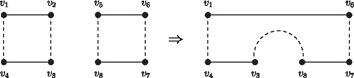
Lemma 3.1 For any two nonadjacent vertices in the odd path graph, their corresponding odd paths can be joined into a cycle by two fusions, one of which is a nongood fusion and the other is a good fusion.

Proof. Let u and v be two nonadjacent vertices in the odd path graph and let p_x_1,y1 and p_x_2,y2 be their corresponding odd paths, respectively, in the adjacent graph. Since u and v are not adjacent, x₁ and x₂ are not the telomeres of the same contig and neither are y₁ and y₂. Then we can use a nongood fusion to join p_x_1,y1 and p_x_2,y2 into a longer path p, which can be either p_x_1,x2 or p_y_1,y2. Clearly, p is a good path, since its length is even and its ends are the telomeres in two different contigs. Therefore, p can be further closed as a cycle by a good fusion. ■

According to Lemma 3.1, we can arbitrarily choose two nonadjacent vertices u and v in the odd path graph G and use two fusions to join their corresponding odd paths, say p₁ and p₂, into a cycle. These two nonadjacent vertices u and v may come from the same alternating cycle or two different alternating cycles in G. If both u and v are in the same alternating cycle of G, say C, then after joining p₁ and p₂, either the length of C will be shortened by two, or C will become two smaller alternating cycles C₁ and C₂ with the sum of their lengths equal to the length of C minus two, that is, |C₁| +|C₂|=|C|−2 (Fig. 6). If u and v belong to different alternating cycles of G, say C₁ and C₂, then after the join of p₁ and p₂, these two alternating cycles will be merged together into a new alternating cycle, say C, whose length is equal to the sum of the lengths of C₁ and C₂ minus two, that is, |C|=|C₁|+|C₂|−2 (Fig. 7). In other words, joining two odds paths, which correspond to two nonadjacent vertices in the odd path graph, into a cycle will decrease the sum of the lengths of all the alternating cycles by two. Therefore, we have the following lemma immediately.

FIG. 6.

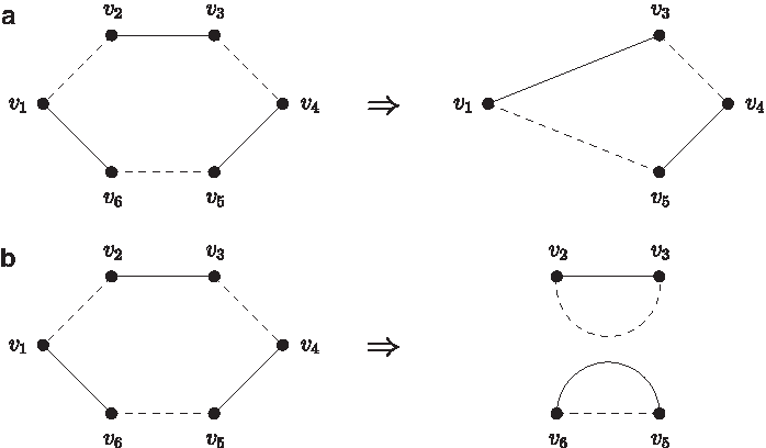
The result obtained by joining two odd paths, which correspond to two nonadjacent vertices u and v in an alternating cycle, into a cycle, where (a) u=v₂ and v=v₆, and (b) u=v₁ and v=v₄.

FIG. 7.

The result obtained by joining two odd paths, which correspond to two nonadjacent vertices u and v in two different alternating cycles, into a cycle, where u=v₂ and v=v₅.

Lemma 3.2 For any two nonadjacent vertices in the odd path graph, joining their corresponding odd paths into a cycle by two fusions decreases the sum of the lengths of all the alternating cycles by two.

Based on Lemmas 3.1 and 3.2, we can repeatedly choose any two nonadjacent vertices from the odd path graph and use two fusions to join their corresponding odd paths into a cycle, until the odd path graph becomes an alternating cycle of length two. After that, if there remain nongood even paths in the resulting adjacent graph, then these non-good even paths can be arbitrarily joined with the two odd paths, which correspond to the vertices of the alternating cycle in the final odd path graph, into two longer odd paths. Finally, these two longer odd paths are joined together into a cycle, if the draft genomes π and σ are circular chromosomes.

Our approach described above can be implemented very efficiently using the techniques of the permutation groups in algebra, because Feijão and Meidanis (2013) have demonstrated that there is a direct relationship between the adjacency graph AG(π,σ) and the permutation \documentclass{aastex}\usepackage{amsbsy}\usepackage{amsfonts}\usepackage{amssymb}\usepackage{bm}\usepackage{mathrsfs}\usepackage{pifont}\usepackage{stmaryrd}\usepackage{textcomp}\usepackage{portland, xspace}\usepackage{amsmath, amsxtra}\pagestyle{empty}\DeclareMathSizes{10}{9}{7}{6}\begin{document} $$\sigma_{ \rm chr} \pi_{ \rm chr}^{ - 1}$$ \end{document} (or, equivalently, \documentclass{aastex}\usepackage{amsbsy}\usepackage{amsfonts}\usepackage{amssymb}\usepackage{bm}\usepackage{mathrsfs}\usepackage{pifont}\usepackage{stmaryrd}\usepackage{textcomp}\usepackage{portland, xspace}\usepackage{amsmath, amsxtra}\pagestyle{empty}\DeclareMathSizes{10}{9}{7}{6}\begin{document} $$\sigma_{ \rm adj} \pi_{ \rm adj}^{ - 1}$$ \end{document} ), as described as the following lemmas. It should be noted that for a draft genome, say π, we will write π_chr as π for simplicity in the rest of this section, that is the notations π and π_chr are interchangeable.

Lemma 3.3 (Feijão and Meidanis, 2013) A cycle of size k, where k is an even integer, in AG(π,σ) contains {e₁,e₂},{e₂,e₃},…,{e_k₋₁,e_k},{e_k,e₁} as vertices, starting with an adjacency {e₁,e₂} in π and alternating adjacencies in π and σ, if and only if (e₁,e₃,…,e_k₋₃,e_k₋₁) and (e_k,e_k₋₂,…,e₄,e₂) are two disjoint cycles in σπ⁻¹.

Lemma 3.4 (Feijão and Meidanis, 2013) An odd path of size k in AG(π,σ) contains {e₁},{e₁,e₂},{e₂,e₃}…,{e_k_-1,e_k},{e_k} as vertices, starting with a telomere {e₁} in π and ending at a telomere {e_n} in σ, if and only if (e_k,e_k₋₂,…,e₃,e₁,e₂,e₄,…,e_k₋₃,e_k_-1) is a cycle in σπ⁻¹.

Lemma 3.5 (Feijão and Meidanis, 2013) An even path of size k in AG(π,σ) contains {e₁},{e₁,e₂},{e₂,e₃}…,{e_k₋₁,e_k},{e_k} as vertices, starting with a telomere {e₁} in π and ending at a telomere {e_n} in π, if and only if (e_k₋₁,e_k₋₃,…,e₃,e₁,e₂,e₄,…,e_k₋₂,e_k) is a cycle in σπ⁻¹.

Lemma 3.6 (Feijão and Meidanis, 2013) An even path of size k in AG(π,σ) contains {e₁},{e₁,e₂},{e₂,e₃}…,{e_k₋₁,e_k},{e_k} as vertices, with starting with a telomere {e₁} in σ and ending at a telomere {e_n} in σ, if and only if (e_k,e_k₋₂,…,e₄,e₂,e₁,e₃,…,e_k₋₃,e_k₋₁) is a cycle in σπ⁻¹.

According to Lemma 3.3, any cycle of size k in AG(π,σ) corresponds to two disjoint \documentclass{aastex}\usepackage{amsbsy}\usepackage{amsfonts}\usepackage{amssymb}\usepackage{bm}\usepackage{mathrsfs}\usepackage{pifont}\usepackage{stmaryrd}\usepackage{textcomp}\usepackage{portland, xspace}\usepackage{amsmath, amsxtra}\pagestyle{empty}\DeclareMathSizes{10}{9}{7}{6}\begin{document} $$ \frac {k} {2} $$ \end{document} -cycles in σπ⁻¹, and according to Lemmas 3.4, 3.5, and 3.6, any path of size k in AG(π,σ) corresponds to a k-cycle in σπ⁻¹. For example, consider the two draft genomes π={[1, 4], [3, 2], [−5, 6], [7, 8]} and σ={[1, 2, 3], [4, 5], [6, 7, 8]}, whose adjacency graph is shown in Figure 3. Then we have π=(1, 4, −4, −1)(3, 2, −2, −3)(−5, 6, −6, 5)(7, 8, −8, −7) and σ=(1, 2, 3, −3, −2, −1)(4, 5, −5, −4)(6, 7, 8, −8, −7, −6) in the chromosomal algebraic representation. Moreover, σπ⁻¹=(1)(−3, −1, 4, 2)(−4, 5, 6)(3, −2)(−5)(−6, 7)(−7)(8)(−8). As depicted in Figure 3, AG(π,σ) has one cycle, simply denoted by c_7h,8t, and seven paths. For these cycle and paths in AG(π,σ), their corresponding cycles in σπ⁻¹ are shown in Table 1.

Table 1.

Corresponding Relationships Between the Paths and Cycles in the Adjacency Graph AG(π,σ) and the Cycles in the Permutation σπ⁻¹

Path or cycle in AG(π,σ)	cycle(s) in σπ⁻¹
p _1t,1t	(1)
p _3h,4t	(−3,−1, 4, 2)
p _4h,6t	(−4, 5, 6)
p _3t,2h	(3,−2)
p _5h,5h	(−5)
p _6h,7t	(−6, 7)
c _7h,8t	(−7)(8)
p _8h,8h	(−8)

In fact, the properties mentioned above are helpful for us to use the operations in the permutation groups to determine whether or not a path in AG(π,σ) is a good path, as described in the following lemmas. Given a set X of contigs, let T(X) denote the set of all telomeres in X.

Lemma 3.7 Let c be a cycle in σπ⁻¹ containing two elements x and y. If x∈T(π),y∈T(π), and (x,y) ∤π, then the path corresponding to c in AG(π,σ) is a good path.

Proof. According to Lemma 3.5, c corresponds to a path, say p, in AG(π,σ) that starts with the telomere {x} in π and ends at the telomere {y} in π. Clearly, p is an even path. Since (x,y) ∤ π, {x} and {y} belong to different contigs in π by Lemma 2.1. Therefore, p is a good path in AG(π,σ). ■

Lemma 3.8 Let c be a cycle in σπ⁻¹ containing two elements x and y. If x∈T(σ),y∈T(σ) and (x,y) ∤ σ, then the path corresponding to c in AG(π,σ) is a good path.

Proof. Basically, πσ⁻¹ can be obtained from σπ⁻¹ by reversing the order of the elements in each cycle of σπ⁻¹, since πσ⁻¹=(σπ⁻¹)⁻¹. In other words, c is a cycle in πσ⁻¹. Since x∈T(σ),y∈T(σ) and (x,y) ∤σ, the path corresponding to c in AG(σ,π) (or, equivalently, AG(π,σ)) is a good path according to Lemma 3.7. ■

For example, consider the draft genomes π and σ as exemplified previously (also refer to Figure 3 and Table 1). The path p_6h,7t in AG(π,σ), which corresponds to the cycle (−6, 7) in σπ⁻¹, is a good path by Lemma 3.7, since −6∈T(π), 7∈T(π) and (−6, 7) ∤ π. However, p_3t,2h in AG(π,σ) is not a good path, since in its corresponding cycle (3,−2) in σπ⁻¹, we have 3∈T(π) and−2∈T(π), but (3,−2)|π. Similarly, p_3h,4t is a good path in AG(π,σ) according to Lemma 3.8, since it corresponds to the cycle (−3,−1, 4, 2) in σπ⁻¹ with −3∈T(σ), 4∈T(σ) and (−3, 4) ∤σ.

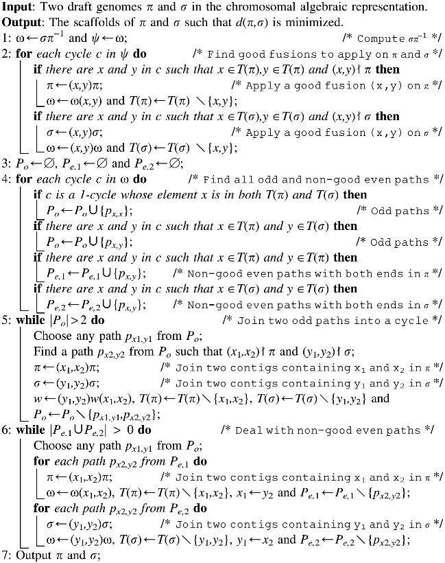
According to the discussion above, we design Algorithm 1 to solve the contig ordering problem for two draft genomes π and σ under the algebraic rearrangement distance. For simplicity, π and σ processed in Algorithm 1 are assumed to be linear. If π and σ are two draft genomes of single circular chromosomes, then the linear contigs returned by Algorithm 1 need to be further circularized into circular contigs by simply joining their telomeres.

In the following, we demonstrate Algorithm 1 by considering two linear draft genomes π={[1, 4], [3, 2], [−5, 6], [7, 8]} and σ={[1, 2, 3], [4, 5], [6, 7, 8]}. By the chromosomal algebraic representation, we have π=(1, 4, −4, −1)(3, 2, −2, −3)(−5, 6, −6, 5)(7, 8, −8, −7) and σ=(1, 2, 3, −3, −2, −1)(4, 5, −5, −4)(6, 7, 8, −8, −7, −6). First of all, we compute σπ⁻¹=(−3, −1, 4, 2)(−4, 5, 6)(3, −2)(−6, 7), in which the cycle (−6, 7) contains two telomeres −6 and 7 from π with (−6, 7) ∤π and the cycle (−3, −1, 4, 2) contains two telomeres −3 and 4 from σ with (−3, 4) ∤σ. Hence, we can apply a good fusion (−6, 7) on π that will join contigs [−5, 6] and [7, 8] into a new one [−5, 6, 7, 8], and apply another good fusion (−3, 4) on σ that will join [1, 2, 3] and [4, 5] into [1, 2, 3, 4, 5]. Actually, applying these two good fusions on π and σ correspond to closing two good paths p_6h,7t and p_3h,4t in their adjacency graph AG(π,σ) (refer to Fig. 3). After that, we have new σπ⁻¹=(−3, −1)(4, 2)(−4, 5, 6)(3, −2), from which we cannot find any good fusions to apply on current π={[1, 4], [3, 2], [−5, 6, 7, 8]} and σ={[1, 2, 3, 4, 5], [6, 7, 8]}. However, we can see from current σπ⁻¹ that the corresponding adjacency graph AG(π,σ) contains four odd paths p_1t,1t,p_4h,6t,p_5h,5h, and p_8h,8h, as well as a nongood even path p_3t,2h. The odd path graph created by p_1t,1t,p_4h,6t,p_5h,5h, and p_8h,8h is equivalent to that as shown in Figure 5. Next, we choose any one from these four odd paths, say p_4h,6t, and find another one p_5h,5h that is not adjacent to p_4h,6t in the odd path graph (since (−4, −5) ∤π and (6,−5) ∤σ). Hence, we can apply (−4, −5) on π to join two contigs [1, 4] and [−5, 6, 7, 8] into a new one [1, 4, −5, 6, 7, 8] and apply (6, −5) on σ to join [1, 2, 3, 4, 5] and [6, 7, 8] into [1, 2, 3, 4, 5, 6, 7, 8]. This is equivalent to joining the two paths p_4h,6t and p_5h,5h in current AG(π,σ) into a cycle. We now have new σπ⁻¹=(6, −4)(5,−5)(−3, −1)(4, 2)(3, −2), in which (3, −2) corresponds to the nongood even path p_3t,2h in AG(π,σ). Then we choose any one of two remaining odd paths, say p_1t,1t, and apply (3, 1) on π, which will join contigs [3, 2] and [1, 4, −5, 6, 7, 8] into a new one [−2, −3, 1, 4, −5, 6, 7, 8]. This action is equivalent to joining p_3t,2h and p_1t,1t in AG(π,σ) into a longer path p_2h,1t. As a result, we finally obtain the scaffolds π={[−2, −3, 1, 4, −5, 6, 7, 8]} and σ={[1, 2, 3, 4, 5, 6, 7, 8]}, and their algebraic rearrangement distance is \documentclass{aastex}\usepackage{amsbsy}\usepackage{amsfonts}\usepackage{amssymb}\usepackage{bm}\usepackage{mathrsfs}\usepackage{pifont}\usepackage{stmaryrd}\usepackage{textcomp}\usepackage{portland, xspace}\usepackage{amsmath, amsxtra}\pagestyle{empty}\DeclareMathSizes{10}{9}{7}{6}\begin{document} $$d ( \pi , \sigma ) = \frac { \parallel \sigma \pi^ { - 1 } \parallel } { 2 } = 3$$ \end{document} .

Algorithm 1.

Theorem 3.1 Given two draft genomes π and σ, the contig ordering problem under the algebraic rearrangement distance can be solved by Algorithm 1 in \documentclass{aastex}\usepackage{amsbsy}\usepackage{amsfonts}\usepackage{amssymb}\usepackage{bm}\usepackage{mathrsfs}\usepackage{pifont}\usepackage{stmaryrd}\usepackage{textcomp}\usepackage{portland, xspace}\usepackage{amsmath, amsxtra}\pagestyle{empty}\DeclareMathSizes{10}{9}{7}{6}\begin{document} $${ \cal O}$$ \end{document} (nf (n)) time, where n is the number of genes and f (n) is the inverse of Ackermann's function.

Proof. The correctness of Algorithm 1 can be justified based on our previous discussion in this section. Below, we analyze the time complexity of Algorithm 1. The computation of σπ⁻¹ in step 1 can be done in \documentclass{aastex}\usepackage{amsbsy}\usepackage{amsfonts}\usepackage{amssymb}\usepackage{bm}\usepackage{mathrsfs}\usepackage{pifont}\usepackage{stmaryrd}\usepackage{textcomp}\usepackage{portland, xspace}\usepackage{amsmath, amsxtra}\pagestyle{empty}\DeclareMathSizes{10}{9}{7}{6}\begin{document} $${ \cal O}$$ \end{document} (n) time. Since ψ contains at most \documentclass{aastex}\usepackage{amsbsy}\usepackage{amsfonts}\usepackage{amssymb}\usepackage{bm}\usepackage{mathrsfs}\usepackage{pifont}\usepackage{stmaryrd}\usepackage{textcomp}\usepackage{portland, xspace}\usepackage{amsmath, amsxtra}\pagestyle{empty}\DeclareMathSizes{10}{9}{7}{6}\begin{document} $$\lfloor \frac { n } { 2 } \rfloor$$ \end{document} disjoint k-cycles, where k≥2, there are at most \documentclass{aastex}\usepackage{amsbsy}\usepackage{amsfonts}\usepackage{amssymb}\usepackage{bm}\usepackage{mathrsfs}\usepackage{pifont}\usepackage{stmaryrd}\usepackage{textcomp}\usepackage{portland, xspace}\usepackage{amsmath, amsxtra}\pagestyle{empty}\DeclareMathSizes{10}{9}{7}{6}\begin{document} $$\lfloor \frac { n } { 2 } \rfloor$$ \end{document} iterations to be performed in step 2. Each iteration in step 2 is to join two contigs in current π or σ by determining whether there are two telomeres x and y from π or σ in each cycle of ψ such that (x,y) ∤π or (x,y) ∤σ. By linearly scanning all the elements in each cycle of ψ, we can find whether this cycle contains two telomeres x and y from π or σ. If so, we can further determine whether or not (x,y) ∤π or (x,y) ∤σ by using the property described in Lemma 2.1. For example, if both x and y appear in a cycle of π, then (x,y)|π; otherwise, (x,y) ∤π. To facilitate computation, we can represent the cycles in π (or σ) as disjoint sets and use two find operations to see whether the set containing x is equal to that containing y. If these two sets are different, then at the next operation, we can use a union operation to merge them into a new set, which corresponds to a good fusion of the two corresponding contigs. The whole process of step 2 requires \documentclass{aastex}\usepackage{amsbsy}\usepackage{amsfonts}\usepackage{amssymb}\usepackage{bm}\usepackage{mathrsfs}\usepackage{pifont}\usepackage{stmaryrd}\usepackage{textcomp}\usepackage{portland, xspace}\usepackage{amsmath, amsxtra}\pagestyle{empty}\DeclareMathSizes{10}{9}{7}{6}\begin{document} $${ \cal O}$$ \end{document} (n) find and \documentclass{aastex}\usepackage{amsbsy}\usepackage{amsfonts}\usepackage{amssymb}\usepackage{bm}\usepackage{mathrsfs}\usepackage{pifont}\usepackage{stmaryrd}\usepackage{textcomp}\usepackage{portland, xspace}\usepackage{amsmath, amsxtra}\pagestyle{empty}\DeclareMathSizes{10}{9}{7}{6}\begin{document} $${ \cal O}$$ \end{document} (n) union operations, which can be implemented by using the so-called disjoint-set data structure in \documentclass{aastex}\usepackage{amsbsy}\usepackage{amsfonts}\usepackage{amssymb}\usepackage{bm}\usepackage{mathrsfs}\usepackage{pifont}\usepackage{stmaryrd}\usepackage{textcomp}\usepackage{portland, xspace}\usepackage{amsmath, amsxtra}\pagestyle{empty}\DeclareMathSizes{10}{9}{7}{6}\begin{document} $${ \cal O}$$ \end{document} (nf (n)) time (Cormen et al., 2009, pp. 561–572), where f (n) is the inverse of Ackermann's function. For step 3, its operations require only constant time. Step 4, which is to find all odd and nongood even paths in the current adjacency graph, can be finished in \documentclass{aastex}\usepackage{amsbsy}\usepackage{amsfonts}\usepackage{amssymb}\usepackage{bm}\usepackage{mathrsfs}\usepackage{pifont}\usepackage{stmaryrd}\usepackage{textcomp}\usepackage{portland, xspace}\usepackage{amsmath, amsxtra}\pagestyle{empty}\DeclareMathSizes{10}{9}{7}{6}\begin{document} $${ \cal O}$$ \end{document} (n) time, since step 4 has at most \documentclass{aastex}\usepackage{amsbsy}\usepackage{amsfonts}\usepackage{amssymb}\usepackage{bm}\usepackage{mathrsfs}\usepackage{pifont}\usepackage{stmaryrd}\usepackage{textcomp}\usepackage{portland, xspace}\usepackage{amsmath, amsxtra}\pagestyle{empty}\DeclareMathSizes{10}{9}{7}{6}\begin{document} $${ \cal O}$$ \end{document} (n) iterations with each iteration taking the time proportional to the length of the corresponding cycle in ω. As to step 5, it is to find two nonadjacent vertices in the odd path graph and join their corresponding odd paths into a cycle. Since the odd path graph has \documentclass{aastex}\usepackage{amsbsy}\usepackage{amsfonts}\usepackage{amssymb}\usepackage{bm}\usepackage{mathrsfs}\usepackage{pifont}\usepackage{stmaryrd}\usepackage{textcomp}\usepackage{portland, xspace}\usepackage{amsmath, amsxtra}\pagestyle{empty}\DeclareMathSizes{10}{9}{7}{6}\begin{document} $${ \cal O}$$ \end{document} (n) vertices, there are \documentclass{aastex}\usepackage{amsbsy}\usepackage{amsfonts}\usepackage{amssymb}\usepackage{bm}\usepackage{mathrsfs}\usepackage{pifont}\usepackage{stmaryrd}\usepackage{textcomp}\usepackage{portland, xspace}\usepackage{amsmath, amsxtra}\pagestyle{empty}\DeclareMathSizes{10}{9}{7}{6}\begin{document} $${ \cal O}$$ \end{document} (n) iterations in step 5. Recall that each vertex in the odd path graph has degree two. Hence, for any p_x_1,y1 of P_o in each iteration of step 5, we need to only check at most three other elements in P_o to find the p_x_2,y2 satisfying (x₁,x₂) ∤π and (y₁,y₂) ∤σ. Again, we can use the disjoint set data structure to implement step 5, which totally requires \documentclass{aastex}\usepackage{amsbsy}\usepackage{amsfonts}\usepackage{amssymb}\usepackage{bm}\usepackage{mathrsfs}\usepackage{pifont}\usepackage{stmaryrd}\usepackage{textcomp}\usepackage{portland, xspace}\usepackage{amsmath, amsxtra}\pagestyle{empty}\DeclareMathSizes{10}{9}{7}{6}\begin{document} $${ \cal O}$$ \end{document} (n) find and \documentclass{aastex}\usepackage{amsbsy}\usepackage{amsfonts}\usepackage{amssymb}\usepackage{bm}\usepackage{mathrsfs}\usepackage{pifont}\usepackage{stmaryrd}\usepackage{textcomp}\usepackage{portland, xspace}\usepackage{amsmath, amsxtra}\pagestyle{empty}\DeclareMathSizes{10}{9}{7}{6}\begin{document} $${ \cal O}$$ \end{document} (n) union operations. Hence, the cost of step 5 is \documentclass{aastex}\usepackage{amsbsy}\usepackage{amsfonts}\usepackage{amssymb}\usepackage{bm}\usepackage{mathrsfs}\usepackage{pifont}\usepackage{stmaryrd}\usepackage{textcomp}\usepackage{portland, xspace}\usepackage{amsmath, amsxtra}\pagestyle{empty}\DeclareMathSizes{10}{9}{7}{6}\begin{document} $${ \cal O}$$ \end{document} (nf (n)). Step 6 deals with nongood even paths by joining them with an odd path. There are \documentclass{aastex}\usepackage{amsbsy}\usepackage{amsfonts}\usepackage{amssymb}\usepackage{bm}\usepackage{mathrsfs}\usepackage{pifont}\usepackage{stmaryrd}\usepackage{textcomp}\usepackage{portland, xspace}\usepackage{amsmath, amsxtra}\pagestyle{empty}\DeclareMathSizes{10}{9}{7}{6}\begin{document} $${ \cal O}$$ \end{document} (n) such joins, with each join taking constant time. Hence, the cost of step 6 is \documentclass{aastex}\usepackage{amsbsy}\usepackage{amsfonts}\usepackage{amssymb}\usepackage{bm}\usepackage{mathrsfs}\usepackage{pifont}\usepackage{stmaryrd}\usepackage{textcomp}\usepackage{portland, xspace}\usepackage{amsmath, amsxtra}\pagestyle{empty}\DeclareMathSizes{10}{9}{7}{6}\begin{document} $${ \cal O}$$ \end{document} (n). Clearly, step 7 requires constant time. As a result, the time complexity of Algorithm 1 is \documentclass{aastex}\usepackage{amsbsy}\usepackage{amsfonts}\usepackage{amssymb}\usepackage{bm}\usepackage{mathrsfs}\usepackage{pifont}\usepackage{stmaryrd}\usepackage{textcomp}\usepackage{portland, xspace}\usepackage{amsmath, amsxtra}\pagestyle{empty}\DeclareMathSizes{10}{9}{7}{6}\begin{document} $${ \cal O}$$ \end{document} (nf (n)). ■

In fact, the time complexity of Algorithm 1 mentioned in Theorem 3.1 is near linear in n, since f (n) is a very slowly growing function. Particularly, f (n)≤4 for all practical purposes (Cormen et al., 2009, pp. 561–572), suggesting that the running time of Algorithm 1 can be considered as linear in n in all practical situations.

4. Conclusions

In this work, we studied the contig ordering problem that aims at ordering and orienting the contigs of two input draft genomes such that the genome rearrangement distance between the resulting scaffolds of the draft genomes is minimized. As a result, we presented a near-linear time algorithm to solve this problem under the algebraic rearrangement distance based on the techniques of permutation groups in algebra and the usage of the disjoint set data structure. It is worth mentioning that our algorithm can be done in linear time for all practical situations. The implementation of this algorithm should have a useful application in genome resequencing, especially when only draft genomes (i.e., unfinished genomes) of organisms related to the genome being sequenced are available for reference or comparison.

Author Disclosure Statement

No competing financial interests exist.

References

Assefa

, Keane

T.M.

, Otto

T.D.

, et al. 2009. ABACAS: algorithm-based automatic contiguation of assembled sequences. Bioinformatics., 25, 1968–1969.

Bentley

D.R.

2006. Whole-genome re-sequencing. Curr. Opin. Genet. Dev., 16, 545–552.

Bergeron

, Mixtacki

, and Stoye

2006. A unifying view of genome rearrangements. Lect. Notes Comput. Sci., 4175, 163–173.

Cormen

T.H.

, Leiserson

, Rivest

, and Stein

2009. Introduction to Algorithms, 3rd edition. MIT Press, Cambridge, MA.

Dias

, Dias

, and Setubal

J.C.

2012. SIS: a program to generate draft genome sequence scaffolds for prokaryotes. BMC Bioinform., 13, 96.

Feijão

, and Meidanis

2013. Extending the algebraic formalism for genome rearrangements to include linear chromosomes. IEEE-ACM Trans. Comput. Biol. Bioinform., 10, 819–831.

Galardini

, Biondi

E.G.

, Bazzicalupo

, and Mengoni

2011. CONTIGuator: a bacterial genomes finishing tool for structural insights on draft genomes. Source Code Biol. Med., 6, 11.

Gaul

, and Blanchette

2006. Ordering partially assembled genomes using gene arrangements. Lect. Notes Comput. Sci., 4205, 113–128.

Huang

Y.-L.

, and Lu

C.L.

2010. Sorting by reversals, generalized transpositions, and translocations using permutation groups. J. Comput. Biol., 17, 685–705.

10.

Husemann

, and Stoye

2010. r2cat: synteny plots and comparative assembly. Bioinformatics., 26, 570–571.

11.

C.-L.

, Chen

K.-T.

, and Lu

C.L.

2013. Assembling contigs in draft genomes using reversals and block-interchanges. BMC Bioinform., 14, S9.

12.

C.L.

, Chen

K.T.

, Huang

S.Y.

, and Chiu

H.T.

2014. CAR: contig assembly of prokaryotic draft genomes using rearrangements. BMC Bioinform., 15, 381.

13.

C.L.

, Huang

Y.-L.

, Wang

T.C.

, and Chiu

H.-T.

2006. Analysis of circular genome rearrangement by fusions, fissions and block-interchanges. BMC Bioinform., 7, 295.

14.

Meidanis

, and Dias

2000. An alternative algebraic formalism for genome rearrangements, 213–223. In Sankoff

, and Nadeau

J.H.

, eds. Comparative Genomics: Empirical and Analytical Approaches to Gene Order Dynamics, Map Alignment and Evolution of Gene Families. Kluwer Academic Press, Amsterdam.

15.

Metzker

M.L.

2010. Sequencing technologies—the next generation. Nat. Rev. Genet., 11, 31–46.

16.

Muñoz

, Zheng

C.F.

, Zhu

Q.A.

, et al. 2010. Scaffold filling, contig fusion and comparative gene order inference. BMC Bioinform., 11, 304.

17.

Pop

2009. Genome assembly reborn: recent computational challenges. Brief. Bioinform., 10, 354–366.

18.

Richter

D.C.

, Schuster

S.C.

, and Huson

D.H.

2007. OSLay: optimal syntenic layout of unfinished assemblies. Bioinformatics., 23, 1573–1579.

19.

Rissman

A.I.

, Mau

, Biehl

B.S.

, et al. 2009. Reordering contigs of draft genomes using the Mauve Aligner. Bioinformatics., 25, 2071–2073.

20.

Shendure

, and Ji

2008. Next-generation DNA sequencing. Nat. Biotechnol., 26, 1135–1145.

21.

van Dijk

E.L.

, Auger

, Jaszczyszyn

, and Thermes

2014. Ten years of next-generation sequencing technology. Trends Genet., 30, 418–426.

22.

van Hijum

S.A.

, Zomer

A.L.

, Kuipers

O.P.

, and Kok

2005. Projector 2: contig mapping for efficient gap-closure of prokaryotic genome sequence assemblies. Nucleic Acids Res., 33, W560–W566.

23.

Yancopoulos

, Attie

, and Friedberg

2005. Efficient sorting of genomic permutations by translocation, inversion and block interchange. Bioinformatics., 21, 3340–3346.