Inference in High-Dimensional Parameter Space

Abstract

Model parameter inference has become increasingly popular in recent years in the field of computational epidemiology, especially for models with a large number of parameters. Techniques such as Approximate Bayesian Computation (ABC) or maximum/partial likelihoods are commonly used to infer parameters in phenomenological models that best describe some set of data. These techniques rely on efficient exploration of the underlying parameter space, which is difficult in high dimensions, especially if there are correlations between the parameters in the model that may not be known a priori. The aim of this article is to demonstrate the use of the recently invented Adaptive Metropolis algorithm for exploring parameter space in a practical way through the use of a simple epidemiological model.

1. Introduction

Modern disease outbreaks are often accompanied by a wealth of observational data that mathematical biologists use to parameterize their models of disease transmission (Deardon et al., 2010; Conlan et al., 2012; House et al., 2012; Biek et al., 2012). This data may include results of routine or post-mortem tests, movements, or network structure information. This a priori information about the transmission processes allows practitioners to understand the dynamics that drive transmission so that outbreaks can be controlled effectively. The difficulty is incorporating this data into mathematical models that describe the transmission of the disease being studied. This is usually done by sampling parameters from some distribution and comparing the outcome to the observations with the observed (prior) information giving some information on the probability distribution of the parameter values (which may simply be a range of permissible values). Inference techniques based on such prior knowledge, examples of which are Approximate Bayesian Computation (ABC) and maximum a posteriori estimation (MAP), fall into the category of Bayesian inference as the prior knowledge is incorporated into the process of estimating parameters, θ , that best describe some data X as follows: \documentclass{aastex}\usepackage{amsbsy}\usepackage{amsfonts}\usepackage{amssymb}\usepackage{bm}\usepackage{mathrsfs}\usepackage{pifont}\usepackage{stmaryrd}\usepackage{textcomp}\usepackage{portland, xspace}\usepackage{amsmath, amsxtra}\pagestyle{empty}\DeclareMathSizes{10}{9}{7}{6}\begin{document} \begin{align*}P ( \theta \mid X ) = \frac { P ( { \bf X } \mid { \bf \theta } ) P ( { \bf \theta } ) } { P ( { \bf X } ) } \tag { 1 } \end{align*} \end{document}

The term on the left-hand-side is the posterior distribution, the calculation of which is the goal of the inference. On the right-hand-side, the numerator is the product of the likelihood and the prior and the denominator serves to ensure that the posterior PDF integrates to unity.

The process of fitting model parameters to observed data is not without difficulty, as there is no single technique for determining the model parameters that best describe observed data with several techniques recently invented to aid this inference. Additional complexity is involved if there exists some correlation between the parameters in the model as it affects the efficiency of how parameters are sampled. The aim of this article is to demonstrate the use of a novel algorithm (Haario et al., 1999, 2001), called the Adaptive Metropolis algorithm, that takes into account possible correlations without having to store the information on all the sampled parameters, thus increasing the efficiency that the parameter space is explored. We will demonstrate the method using a practical example of inferring the parameters in a simple disease model with several parameters. We will use an algorithmic approach to demonstrate the algorithm with Markov chain maximum a posteriori estimates to demonstrate how this method may be used to estimate the parameters in a disease model. We refer the reader to more theoretical treatments of the techniques in this article to other work (Haario et al., 2001; Gauvin and Lui, 1994; Andrieu and Atchad, 2007).

2. Adaptive Metropolis Algorithm

As a demonstration of the technique we will use the SEIR model without recruitment and with frequency dependent transmission (Equation 2) and recover parameters that create a known outbreak pattern. This model divides a population into four categories—susceptible, S, those who may be infected but currently are not; exposed, E, those that are infected but not able to infect others; infectious, I, those who are able to infect others and finally recovered; and R are those that have had the disease and have recovered. It is assumed, in this model, that individuals pass from S→E→I→R in a linear manner. \documentclass{aastex}\usepackage{amsbsy}\usepackage{amsfonts}\usepackage{amssymb}\usepackage{bm}\usepackage{mathrsfs}\usepackage{pifont}\usepackage{stmaryrd}\usepackage{textcomp}\usepackage{portland, xspace}\usepackage{amsmath, amsxtra}\pagestyle{empty}\DeclareMathSizes{10}{9}{7}{6}\begin{document} \begin{align*} \dot { S } & = - \beta \frac { IS } { N } \\ \dot { E } & = \beta \frac { IS } { N } - \sigma E \\ \dot { I } & = \sigma E - \gamma I \\ \dot { R } & = \gamma I & ( 2 ) \end{align*} \end{document}

We will create the disease pattern by observing the numbers of S, E, I, and R in a population of 10000 individuals. In this rather contrived example we start with S=9999, I=1 with β=0.287, σ=0.67, and γ=0.16, and solve the equations using the fourth order Runge-Kutta method with a step-size of 0.1. At t=100 we record the numbers of susceptible and recovereds as 4583 and 4349, respectively, and record those infected and exposed together as 1068.

Despite its simplicity, this model demonstrates a problem confronting computational epidemiologists; having observed disease data and a phenomenological understanding of the transmission dynamics, what are the transmission parameters? Knowing these parameters allows us to design control measures to combat the spread of the disease.

Firstly, let us write the parameters of the model as θ ={β, σ, γ}, and we wish to determine these parameters based on some observations, X={4583, 1068, 4349}. If we denote p(X) as the probability distribution of the observations X, we can write the probability of observing X given a set of parameters as p(X| θ ). This function is known as the likelihood function. Maximizing this function for a given statistical model and observed data provides a method for estimating the model parameters known as the maximum likelihood (ML) method.

Maximum a posteriori (MAP) estimation is very similar to ML estimation but allows the inclusion of some a priori belief on the parameters by weighting them with a prior distribution p( θ ). MAP, therefore, incorporates a prior distribution to the likelihood to estimate unobserved quantities based on empirical data. It is used to estimate a mode of the posterior distribution (the value of the parameter for which the posterior distribution is a maximum). If we have some knowledge about the distribution of θ , we can treat them as random variables as in Bayesian statistics. This prior knowledge can be as simple as a uniform distribution within some wide limits for priors that are not well known to specific distributions with low measures of spread for well-known priors. The posterior distribution of the parameters given the observed data can now be written as \documentclass{aastex}\usepackage{amsbsy}\usepackage{amsfonts}\usepackage{amssymb}\usepackage{bm}\usepackage{mathrsfs}\usepackage{pifont}\usepackage{stmaryrd}\usepackage{textcomp}\usepackage{portland, xspace}\usepackage{amsmath, amsxtra}\pagestyle{empty}\DeclareMathSizes{10}{9}{7}{6}\begin{document} \begin{align*}P ( { \bf \theta } \mid { \bf X } ) = \frac { P ( { \bf X } \mid { \bf \theta } ) g ( { \bf \theta } ) } { \int_ \vartheta P ( { \bf X } \mid \vartheta ) g ( \vartheta ) { \rm d } \vartheta } \tag { 3 } \end{align*} \end{document}

where the integral in the denominator is over the domain of g, the prior distribution of the parameters θ , and is usually evaluated numerically by sampling the parameters over the prior space. MAP estimates the model parameters, \documentclass{aastex}\usepackage{amsbsy}\usepackage{amsfonts}\usepackage{amssymb}\usepackage{bm}\usepackage{mathrsfs}\usepackage{pifont}\usepackage{stmaryrd}\usepackage{textcomp}\usepackage{portland, xspace}\usepackage{amsmath, amsxtra}\pagestyle{empty}\DeclareMathSizes{10}{9}{7}{6}\begin{document} $$\hat{{ \bf \theta}}$$ \end{document} , for which the posterior distribution has it's maximum (i.e., the mode of the distribution) and is written as \documentclass{aastex}\usepackage{amsbsy}\usepackage{amsfonts}\usepackage{amssymb}\usepackage{bm}\usepackage{mathrsfs}\usepackage{pifont}\usepackage{stmaryrd}\usepackage{textcomp}\usepackage{portland, xspace}\usepackage{amsmath, amsxtra}\pagestyle{empty}\DeclareMathSizes{10}{9}{7}{6}\begin{document} \begin{align*}\hat { { \bf \theta } } _ { \rm MAX } = { \rm argmax } _ { { \bf \theta } } P ( { \bf \theta } \mid { \bf X } ) = { \rm argmax } _ { \bf \theta } \frac { P ( { \bf X } \mid { \bf \theta } ) g ( { \bf \theta } ) } { \int_ \vartheta P ( { \bf X } \mid \vartheta ) g ( \vartheta ) { \rm d } \vartheta } \tag { 4 } \end{align*} \end{document}

Thus our problem is to find those parameters, θ , that maximize the posterior P( θ |X). This is rather straightforward for models in which we know the conditional probabilities P(X| θ ), we can write down the distributions in Equation (4) and find the argmax by differentiating the likelihood, setting the derivative to zero, and solving for θ . For more complex models we need to explore parameter space to find \documentclass{aastex}\usepackage{amsbsy}\usepackage{amsfonts}\usepackage{amssymb}\usepackage{bm}\usepackage{mathrsfs}\usepackage{pifont}\usepackage{stmaryrd}\usepackage{textcomp}\usepackage{portland, xspace}\usepackage{amsmath, amsxtra}\pagestyle{empty}\DeclareMathSizes{10}{9}{7}{6}\begin{document} $$\,\hat{{ \bf \theta}}$$ \end{document} , which can achieved by simulating this distribution using the Markov chain Monte Carlo. Using this technique gives us a distribution for the estimates for \documentclass{aastex}\usepackage{amsbsy}\usepackage{amsfonts}\usepackage{amssymb}\usepackage{bm}\usepackage{mathrsfs}\usepackage{pifont}\usepackage{stmaryrd}\usepackage{textcomp}\usepackage{portland, xspace}\usepackage{amsmath, amsxtra}\pagestyle{empty}\DeclareMathSizes{10}{9}{7}{6}\begin{document} $$\,\hat{{ \bf \theta}}$$ \end{document} rather than the point estimates returned by ML.

Suppose, in our example, we are able to test every individual in a population to determine their disease state for some transmissible disease and were able to categorize these correctly as being susceptible (for example, no antibodies were found in their blood), infected (in either contagious or subcontagious stage), and recovered. Since our test is not capable of determining those in the E class from I in our model, the correlation between σ and γ will need to be taken into account in any method of calculating \documentclass{aastex}\usepackage{amsbsy}\usepackage{amsfonts}\usepackage{amssymb}\usepackage{bm}\usepackage{mathrsfs}\usepackage{pifont}\usepackage{stmaryrd}\usepackage{textcomp}\usepackage{portland, xspace}\usepackage{amsmath, amsxtra}\pagestyle{empty}\DeclareMathSizes{10}{9}{7}{6}\begin{document} $$\,\hat{{ \bf \theta}}_{ \rm MAX}$$ \end{document} .

Calculating the probability in Equation (3) for most models is intractable and is often approximated using Monte Carlo methods, which performs the integration by sampling θ from a distribution and “saving” those samples that satisfy a condition. This (inefficient) Monte Carlo integration is improved by exploring the parameter space in a manner that hones in on the area of space that we want (i.e., gives those parameters that maximize a likelihood function or minimize a distance function in ABC). A Markov chain is an efficient method of walking through parameter space creating a chain of steps that successively reach the required area by taking a trial step and either accepting or rejecting it based on a rejection algorithm. The Markov chain Monte Carlo method is an algorithm that combines the Markov chain and Monte Carlo methods to evaluate integrals such as those in Equation (3). There have been many articles published on MCMC, for example, Gilks et al. (1996), Brooks (1998), and Berthelsen and Møller (2003), which should be consulted for a more rigorous treatment; we will only give an algorithmic outline here.

In this example, we wish to maximize the likelihood \documentclass{aastex}\usepackage{amsbsy}\usepackage{amsfonts}\usepackage{amssymb}\usepackage{bm}\usepackage{mathrsfs}\usepackage{pifont}\usepackage{stmaryrd}\usepackage{textcomp}\usepackage{portland, xspace}\usepackage{amsmath, amsxtra}\pagestyle{empty}\DeclareMathSizes{10}{9}{7}{6}\begin{document} \begin{align*} { \cal L } = \frac { N! } { N_S!N_I!N_R! } p_s^ {N_S} p_I^ {N_I} p_R^ {N_R} \tag {5} \end{align*} \end{document}

where N_S are the numbers of susceptibles observed in the population for the parameters θ , and similarly N_I and N_R are the numbers of infected and recovered. The probabilities p_s, p_I, p_R are the probabilities of observing N_S, N_I, N_R and can be calculated from the proportions of each in the underlying population that we are trying to model. We can think of the likelihood function, in this example, as a surface (albeit in 3D) where our parameters define a location and the likelihood function defines an altitude, the MCMC method thus explores this landscape looking for the highest peak preferring those trial steps that climb rather than descend the local hills.

The steps to perform the MCMC algorithm are:

1. Select a starting point in the parameter space, effectively choose a β, σ, γ from a known distribution. In Bayesian terms this distribution is known as the prior distribution and represents the knowledge we have about these parameters, for example, the range of values they can take and how they are distributed. In this case we will assume very little knowledge and assume a uniform distribution over quite a large range, [0.05, 1.0] for each parameter. The efficiency of this approach is improved if the range can be decreased or a known distribution is used.

2. Calculate the required statistic that is being optimized. In this case we calculate the likelihood from Equation (5). Calculating this statistic is usually the most computationally intensive part of the algorithm as it typically may involve Monte Carlo simulation to obtain the output values (in this case N_S, N_I, N_R).

3. Take a trial step by selecting a new set of parameters θ _trial=β_trial, σ_trial, γ_trial. There is no hard and fast rule about how to select these parameters; taking a large step means the parameter space is explored more quickly but not with any great accuracy; steps that are too small mean that the local area is explored in great detail but it takes longer to explore the whole space. In general, selecting a trial step from a normal distribution makes sense where the standard deviation, ূ, can be used to “tune” the step size [i.e., β_trial∼N(β, ূ_β),σ_trial∼N(σ, ূ_σ), γ_trial∼N(γ, ূ_γ)].

4. Compare the statistic for this trial step to the previous step and accept according to a rejection algorithm, if the trial is accepted the the parameters are updated θ = θ _trial, and a new trial step is sampled; otherwise, the trial step is rejected.

The Metropolis-Hastings algorithm is commonly used to determine whether or not to accept the trial step. The basic algorithm is to compare the statistics of the trial step to the current one ( \documentclass{aastex}\usepackage{amsbsy}\usepackage{amsfonts}\usepackage{amssymb}\usepackage{bm}\usepackage{mathrsfs}\usepackage{pifont}\usepackage{stmaryrd}\usepackage{textcomp}\usepackage{portland, xspace}\usepackage{amsmath, amsxtra}\pagestyle{empty}\DeclareMathSizes{10}{9}{7}{6}\begin{document} $${ \cal L_{ \rm trial}} / { \cal L}$$ \end{document} and accept it if it is less than a random variable drawn from a uniform distribution in the range [0, 1]. If \documentclass{aastex}\usepackage{amsbsy}\usepackage{amsfonts}\usepackage{amssymb}\usepackage{bm}\usepackage{mathrsfs}\usepackage{pifont}\usepackage{stmaryrd}\usepackage{textcomp}\usepackage{portland, xspace}\usepackage{amsmath, amsxtra}\pagestyle{empty}\DeclareMathSizes{10}{9}{7}{6}\begin{document} $${ \cal L_{ \rm trial}} \ge { \cal L}$$ \end{document} then the trial step is always accepted (thus always moving toward the areas of parameter space that maximize the likelihood), conversely if \documentclass{aastex}\usepackage{amsbsy}\usepackage{amsfonts}\usepackage{amssymb}\usepackage{bm}\usepackage{mathrsfs}\usepackage{pifont}\usepackage{stmaryrd}\usepackage{textcomp}\usepackage{portland, xspace}\usepackage{amsmath, amsxtra}\pagestyle{empty}\DeclareMathSizes{10}{9}{7}{6}\begin{document} $${ \cal L_{ \rm trial}} < { \cal L}$$ \end{document} the trial step has a high probability of being accepting if the trial likelihood is close to that of the previous step, allowing a chance of “going downhill.” This means that the walk does not get stuck in a local maximum and thus guarantees that the global maximum will be found (but makes no prediction as to how long it will take to find).

5. This process of making trial step and accepting/rejecting them performs a random walk through parameter space that has the properties of a Markov chain. Several such chains are run, each with a different initial θ until each converge on the same region of the parameter space. This region defines the posterior distribution. The goal of any inference technique is to find this region and draw samples from it, the distribution of these sampled parameters make up the posterior distribution of the parameters.

MCMC will generate parameters while exploring parameter space in a manner that spends the most time in the important regions. In the parlance of inference methods, the samples (parameters) mimic samples drawn from the target distribution (i.e., those parameters we are trying to find).

The efficiency of the MCMC is determined by how well the random walk (Markov chain) explores the parameter space. A frequently used method for choosing a trial step is to sample from a symmetric distribution centerd on the current step (known as the symmetric random walk method, SRWM) as it is easy to implement and is often efficient enough for practical purposes, even for high-dimensional distributions. This is the method outlined in step 3 above using the normal distribution. Finding a good choice of proposal distribution is not an easy task however. For many problems a possible choice is the multivariate normal distribution with means, θ and covariance matrix Γ (called the N-SRWM). The convergence rate of the N-SRWM method—that is, how quickly the random walk converges on the desired region of space, depends on the covariance between parameters used in calculating the trial step. Failure to take the correlations between parameters into account will result in exploring an area of space that will not contribute to the posterior distribution. These correlations can be taken into account when sampling from a multivariate normal distribution by using the covariance matrix for the distribution to calculate the joint probability distribution for the random variables.

In practice this covariance is calculated by storing all the values, θ _i, that make up the chain and is both time and memory intensive. To generate a step in a Markov chain we need to sample from a multivariate normal distribution with a mean \documentclass{aastex}\usepackage{amsbsy}\usepackage{amsfonts}\usepackage{amssymb}\usepackage{bm}\usepackage{mathrsfs}\usepackage{pifont}\usepackage{stmaryrd}\usepackage{textcomp}\usepackage{portland, xspace}\usepackage{amsmath, amsxtra}\pagestyle{empty}\DeclareMathSizes{10}{9}{7}{6}\begin{document} $${ \bf \mu} = \{ \,\hat{ \beta} , \hat{ \sigma} , \hat{ \gamma} \} $$ \end{document} and covariance matrix \documentclass{aastex}\usepackage{amsbsy}\usepackage{amsfonts}\usepackage{amssymb}\usepackage{bm}\usepackage{mathrsfs}\usepackage{pifont}\usepackage{stmaryrd}\usepackage{textcomp}\usepackage{portland, xspace}\usepackage{amsmath, amsxtra}\pagestyle{empty}\DeclareMathSizes{10}{9}{7}{6}\begin{document} \begin{align*}{\bf \Sigma} = \left( \begin{matrix}c_{ \beta \beta} & c_{ \beta \sigma} & c_{ \beta \gamma} \\ c_{ \sigma \beta} & c_{ \sigma \sigma} & c_{ \sigma \gamma} \\ c_{ \gamma \beta} & c_{ \gamma \sigma} & c_{ \gamma \gamma}\end{matrix} \right) \tag{6} \end{align*} \end{document}

where the covariance between the parameters x and y is given by c_xy=E [(x–E[x]) (y–E[y])] (E [x] denotes the expected value of x).

The random samples for our next step θ can be generated from an independent normal samples as \documentclass{aastex}\usepackage{amsbsy}\usepackage{amsfonts}\usepackage{amssymb}\usepackage{bm}\usepackage{mathrsfs}\usepackage{pifont}\usepackage{stmaryrd}\usepackage{textcomp}\usepackage{portland, xspace}\usepackage{amsmath, amsxtra}\pagestyle{empty}\DeclareMathSizes{10}{9}{7}{6}\begin{document} \begin{align*} {\bf \theta} = {\bf \mu} + {\bf LN} \tag{7} \end{align*} \end{document}

where N is a vector of independent and identically drawn (iid) N(0, 1) random variables, and L is the solution to Σ=LL′ (the Cholesky factorization of Σ). To draw these samples we need to store the parameters for each step of the Markov chain, which is a problem as these chains are typically long and calculating the L matrix can be computationally intensive. Unfortunately, the trade-off between the faster convergence rate and the calculation of the covariance matrix at each step in the chain is found by trial and error.

Haario et al. (1999, 2001) proposed a novel method, referred to as the Adaptive Metropolis algorithm, to replace the costly calculation of the covariance matrix by updating the matrix on-the-fly using only the current k-th step in the chain and the previous μ and Γ as \documentclass{aastex}\usepackage{amsbsy}\usepackage{amsfonts}\usepackage{amssymb}\usepackage{bm}\usepackage{mathrsfs}\usepackage{pifont}\usepackage{stmaryrd}\usepackage{textcomp}\usepackage{portland, xspace}\usepackage{amsmath, amsxtra}\pagestyle{empty}\DeclareMathSizes{10}{9}{7}{6}\begin{document} \begin{align*} { \bf \mu } _ { k + 1 } & = { \bf \mu } _k + \frac { 1 } { k + 1 } \left( { \bf \theta } _ { k + 1 } - { \bf \mu } _k \right) \\ { \bf \Gamma } _ { k + 1 } & = { \bf \Gamma } _k + \frac { 1 } { k + 1 } \Big ( \left( { \bf \theta } _ { k + 1 } - { \bf \mu } _k \right) \left( { \bf \theta } _ { k + 1 } - { \bf \mu } _k \right) ^T - \Gamma_k \Big) \tag { 8 }\end{align*} \end{document}

with the parameters being drawn from the multivariate distribution θ _k+1∼N( μ _k, Γ_k).

To compare the SRWM, N-SRWM, and Adaptive Metropolis algorithm, we will infer the parameters in our SEIR model from a set of observed data. We create the observed data by running the SEIR model with β=0.287, σ=0.67, γ=0.16, and S₀=9999, E₀=0, i₀=1, R₀=0 for t=[0, 1] with a step size of 0.1 using the 4^th order Runge-Kutta. This resulted in S=4583, R=4349, E+I=1068.

For each algorithm we start with θ ={β=0.387, σ=0.17, γ=0.46} and use the three inference techniques described above to maximize the likelihood in Equation (5). For the SRWM sample the new step is drawn from N ( θ , 1) (this is quite large and normally a degree of tuning is required to find an optimal value). For the N-SRWM we sample, the new step is drawn from N ( θ , I ). This also is suboptimal as the correlations are ignored, but for this purpose we will ignore correlations and note that the results for the N-SRWM will not be as efficient as they could. The new step for the Adaptive Metropolis algorithm is chosen by updating the covariance matrix at each step according to Equation (8) and summarized by the following algorithm:

1. Let θ_i be the coordinates of the current step (so θ₁=β, θ₂=σ, θ₃=γ) and μ_k be the mean values of the parameters after the k-th step ( \documentclass{aastex}\usepackage{amsbsy}\usepackage{amsfonts}\usepackage{amssymb}\usepackage{bm}\usepackage{mathrsfs}\usepackage{pifont}\usepackage{stmaryrd}\usepackage{textcomp}\usepackage{portland, xspace}\usepackage{amsmath, amsxtra}\pagestyle{empty}\DeclareMathSizes{10}{9}{7}{6}\begin{document} $$\mu_k = \{ \,\hat{ \beta} , \hat{ \sigma} , \hat{ \gamma} \} $$ \end{document} ) update the means according to Equation (8) \documentclass{aastex}\usepackage{amsbsy}\usepackage{amsfonts}\usepackage{amssymb}\usepackage{bm}\usepackage{mathrsfs}\usepackage{pifont}\usepackage{stmaryrd}\usepackage{textcomp}\usepackage{portland, xspace}\usepackage{amsmath, amsxtra}\pagestyle{empty}\DeclareMathSizes{10}{9}{7}{6}\begin{document} \begin{align*} \mu_ \beta & = \mu_ \beta + \frac { \beta - \mu_ \beta } { k + 1 } \\ \mu_ \sigma & = \mu_ \sigma + \frac { \sigma - \mu_ \sigma } { k + 1 } \\ \mu_ \gamma & = \mu_ \gamma + \frac { \gamma - \mu_ \gamma } { k + 1 } & ( 9 ) \end{align*} \end{document}

2. Update the covariance matrix Γ according to Equation (8). Let i, j be the (row,column) coordinates of the matrix then \documentclass{aastex}\usepackage{amsbsy}\usepackage{amsfonts}\usepackage{amssymb}\usepackage{bm}\usepackage{mathrsfs}\usepackage{pifont}\usepackage{stmaryrd}\usepackage{textcomp}\usepackage{portland, xspace}\usepackage{amsmath, amsxtra}\pagestyle{empty}\DeclareMathSizes{10}{9}{7}{6}\begin{document} \begin{align*}\Gamma_ { i , j } = \Gamma_ { i , j } + \frac { \Sigma - \Gamma_ { i , j } } { k + 1 } \end{align*} \end{document}

where \documentclass{aastex}\usepackage{amsbsy}\usepackage{amsfonts}\usepackage{amssymb}\usepackage{bm}\usepackage{mathrsfs}\usepackage{pifont}\usepackage{stmaryrd}\usepackage{textcomp}\usepackage{portland, xspace}\usepackage{amsmath, amsxtra}\pagestyle{empty}\DeclareMathSizes{10}{9}{7}{6}\begin{document} \begin{align*}\Sigma = \left( x_i - \mu_i \right) \times \left( x_j - \mu_j \right)\end{align*} \end{document}

It is possible to obtain a singular matrix using these formulae; to avoid this we can set Γ_i,j=Γ_i,j*ε for some small value ε.

3. Obtain the next step θ ={β, σ, γ} from a multivariate normal distribution using these calculated means and covariances θ ∼N ( μ , Γ).

For each method, we solve the SEIR model in t=[0, 1] with the same initial conditions and stepsize as the model that generated the observed data. (We admit this is rather an artificial construct but enough to demonstrate the method. The goal here is to show how the Adaptive Metropolis algorithm may be used in a Bayesian context). We generate the Markov chain by drawing 150000 samples from the prior distribution of the parameters [U(0.05,1.0) for each parameter].

We can see that the simulations using the Adaptive Metropolis method was the quickest to converge on the posterior distribution (Fig. 1), though once it reaches the target distribution its efficiency in sampling from this distribution decreases. In all the above chains 150,000 samples were drawn, but despite the Adaptive Metropolis algorithm reaching the target distribution quicker than the other two methods it failed to select efficiently from this distribution. The other two methods were, nonetheless, untuned, in that changing the variance used in the sampling strategy (in effect limiting the size of the step) would result in a more efficient exploration of the local environment. Decreasing the variance in these algorithms once the target distribution is identified (often referred to as adaptive or sequential MCMC) would increase the sampling rate from the posterior distribution.

FIG. 1.

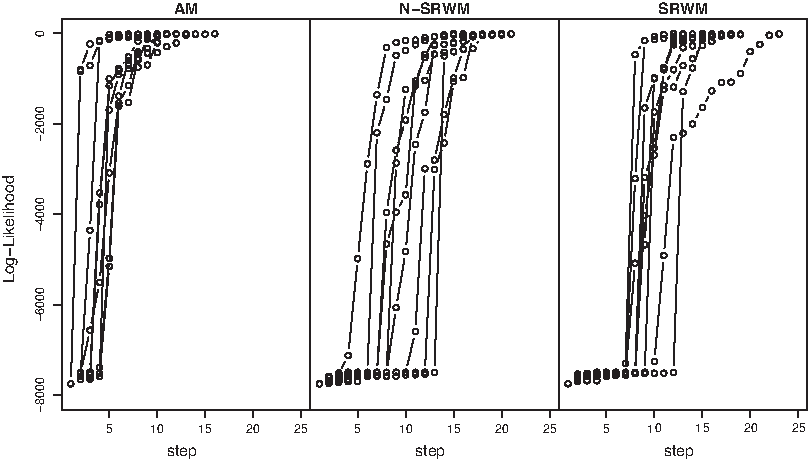
Log-likelihoods for the Markov chain using the Adaptive Metropolis method, N-SRWM, and SRWM algorithms. At each step of the chain the SEIR model was solved using the Runge-Kutta method and the log-likelihood calculated at each step. Each trial step was accepted according to the Metropolis-Hastings algorithm. Convergence is significantly faster for the Adoptive Metropolis algorithm than either of the others.

Due to the inefficiency of the sampling strategies we have only one or two points from each chain from which to obtain the posterior distribution (Fig. 2). In practice this is not enough points to generate a posterior distribution, especially when there are known correlations between the parameters in the underlying model, but we present it here for illustrative purposes. In all inference techniques used the observed values were recovered but the fitted (or inferred) parameter values were not. This is entirely due to the correlations between the parameters, as there is a wide range of {β, σ, γ} that will recreate the observed output. This should serve as a warning on the use of inappropriate priors, if we restricted the range of our priors, or specified a particular distribution for these priors we would have been more successful in obtaining the parameters.

FIG. 2.

Posterior distributions of the parameters for Adaptive Metropolis method, N-SRWM, and SRWM. For each algorithm the chains converged on an area of parameter space that was able to recreate the observed output. Each chain was started with a value of β=0.287, σ=0.67, and γ=0.16 and created from 150000 draws from the sample distribution. The posterior distributions were smoothed using the density() function in R, the statistical computing language.

3. Conclusions

Parameter inference, especially in models with a large number of parameters, is a difficult and time-consuming task. Efficient exploration of the parameter space is key to obtaining good posterior estimates. Identifying and using correlations between the parameter in the fitted models is key to achieving this efficiency, but calculating these correlations comes with an additional computational effort. The Adaptive Metropolis algorithm is an efficient method, in both memory and CPU, to account for these correlations. We have demonstrated that this algorithm is faster than naive SRWM and N-SRWM methods, though these methods may be considerably improved with a degree of tuning obtained by trial and error. The Adaptive Metropolis algorithm requires no tuning to reach the target distribution.

Footnotes

Author Disclosure Statement

No competing financial interests exist.

References

Andrieu

, and Atchad

Y.F.

2007. On the effciency of adaptive MCMC algorithms. Elect. Comm. Probab., 12, 336349.

Berthelsen

K.K.

, and Møller

2003. Likelihood and non-parametric Bayesian MCMC inference for spatial point processes based on perfect simulation and path sampling. Scand. J. Stat., 30, 549564.

Biek

, O'Hare

, Wright

, et al. 2012. Whole genome sequencing reveals local transmission patterns of Mycobacterium bovis in sympatric cattle and badger populations. PLoS Pathogens., 8, e1003008.

Brooks

S.P.

1998. Markov chain Monte Carlo method and its application. Statistician., 47, 69–100.

Conlan

A.J.K.

, Mckinley

T.J.

, Karolemeas

, et al. 2012. Estimating the hidden burden of bovine tuberculosis in Great Britain. PLoS Comp. Biol., 8, e1002730.

Deardon

, Brooks

S.P.

, Grenfell

B.T.

, et al. 2010. Inference for individual-level models of infectious diseases in large populations. Stat. Sin., 20, 239–261.

Gauvin

J.L.

, and Lui

1994. Maximum a posteriori estimation for multivariate Gaussian mixture observations of Markov chains. IEEE Trans. Speech Audio Process., 2, 291–298.

Gilks

W.R.

, et al., eds. 1996. Markov Chain Monte Carlo in Practice. Chapman & Hall, London.

Haario

, Saksman

, and Tamminen

1999. Adaptive proposal distribution for random walk Metropolis algorithm. Comput. Stat., 14, 375395.

10.

Haario

, Saksman

, and Tamminen

2001. An adaptive Metropolis algorithm. Bernoulli., 7, 223242.

11.

House

T.A.

, Inglis

, Ross

J.R.

, et al. 2012. Estimation of outbreak severity and transmissibility: influenza A(H1N1)pdm09 in households. BMC Med., 10, 117.