Detecting Character Dependencies in Stochastic Models of Evolution

1. Introduction

Reconstructing the phylogeny or evolutionary tree of a set of organisms is a very important problem in biology (Felsenstein, 2004; Semple and Steel, 2003). The general formulation of the problem is the following: data corresponding to the species alive today is observed at the leaves of an (unknown) tree that models the evolutionary history of these species. The goal is to find the best tree “fitting the data” under some specified objective function. Nowadays the most common type of data we observe is biomolecular sequences, that is, DNA or protein sequences. Let σ_i be the sequence obtained from the i^th species. These input sequences are aligned, that is, lined up in columns such that for all i, i′, and for any position j, σ_i[j] and σ_i′[j] have a common evolutionary origin, ¹ where σ_i[j] represents the j^th symbol in σ_i.The most principled method of finding a phylogeny is to view the evolution of each position of the aligned DNA sequences as a stochastic process, more specifically, as a tree Markov random field whose parameters are chosen from a rich family of possible parameters.

A tree Markov random field consists of an underlying rooted tree T. A character on such a tree is a stochastic process that takes on a value at each point in the tree from a set of finitely many states. At the root of T the value is assumed to be from some initial distribution over the states. Each parent attempts to pass its state to its children. However, the state is “mutated” along each edge with probabilities given by a Markov transition matrix corresponding to the edge. Every position in a set of aligned molecular sequences is regarded as a character evolving in this manner, and we observe its state at each leaf of the tree. The tree itself is unknown. Using the maximum likelihood objective function, the goal is to reconstruct the tree and most likely the values of the parameters given the observed data at the leaves (Felsenstein, 1981; Huelsenbeck and Crandall, 1997). Under standard stochastic models of the evolutionary process and reasonable technical constraints on the transition matrices, considerable work has been done to determine the number of characters needed to infer the phylogeny. (Chang, 1996; Daskalakis et al., 2006; Erdos et al., 1999; Erdös et al., 1999; Farach and Kannan, 1999; Goldman, 1998; Mossel, 2004a; Mossel and Roch, 2005). All of these works assume that the stochastic processes governing each character are independent and identically distributed.

The independence assumption across characters is too strong. Dependence between characters arises because changes at one position of a DNA sequence or amino acid sequence are likely to be correlated with changes at other positions because of constraints on size, charge, hydrophobicity, etc., of the molecules involved (Morcos et al., 2011, 2013). The double-helical structure of the DNA and the fact that each turn of the double helix corresponds to roughly seven nucleotides means that there are likely to be dependencies between a character and another that is seven positions away. Similarly, the three-dimensional conformation of protein molecules imposes dependencies between spatially adjacent amino acids. Maddison (1990) and the references cited therein outline simple heuristic procedures. Previous work has acknowledged the possible dependence from sources such as the above, and work has been done in detecting correlations between pairs of characters in Schöniger and Von Haeseler (1994) and Tillier and Collins (1995). Many authors have also used likelihood ratio tests for detecting dependence, taking advantage of some prior knowledge of the phylogenetic tree (Felsenstein and Churchill, 1996; Pagel, 1994).

In this article we reconsider the question: Given two such characters, can we decide if they are independent? Our answer is yes, under biologically reasonable assumptions about the tree Markov random field (that is the model of evolution) and the type of dependence allowed. In this work, we show a proof of concept that dependence can be detected using just census data, though we make no claims to the statistical efficiency of this approach, compared to the likelihood tests mentioned above. We note that there are problems such as the reconstruction problem on trees in the Ising model, where a census is a sufficient statistic (Mossel, 2004b).

All commonly studied families of stochastic models of evolution are tree Markov random fields. Among the simplest are two-state, symmetric models, called the Cavender–Farris–Neyman (CFN) (Cavender, 1978; Farris, 1973; Neyman, (1971) models, where on any edge e, all characters have a symmetric 2 × 2 transition matrix M_e. The Jukes–Cantor model is a four-state model where for any transition matrix there is a parameter ɛ that is the probability of any change of state (Jukes and Cantor, 1969). In this article, we will look at a range of models of evolution to address the question above; even the most restrictive model we consider in this article is more general than these standard biological models.

In addition, we introduce some simple models of dependence among characters that seem well-suited to the biological application. The definition of these models themselves is one of the main contributions of this article. If two characters are independent, then on each edge of the tree the matrix governing their joint evolution is just the tensor product of the marginal matrices. Two characters are dependent if this does not hold, that is, if there are edges where the transition matrix for the joint character differs (significantly) from the tensor product of the marginals. Thus, dependence of two characters is captured by their joint transition matrix M deviating significantly from the tensor product T of their marginal matrices. The difference between the i^th rows of M and T is the difference in next-state probabilities when the process is in the joint state, i. If there is a biological reason that certain next-states are preferred, this reason should persist across all the rows of the deviation matrix, M – T. Thus, we expect all rows of M – T to point roughly in the same direction. Similarly, this biological reason should persist throughout the phylogeny, and hence we expect deviations on each edge of the tree to also point in roughly the same direction. This is just as well because, mathematically, it would be impossible to detect dependencies when the deviations on different edges could potentially cancel out the dependence signal. Our bounds on how well we can detect dependence are a function of how well aligned the deviation vectors are to some specific direction.

Another remark is in order about our restriction to detecting dependence of pairs of characters. In biologically realistic scenarios even dependencies across sets of characters of cardinality greater than two will manifest as dependencies of pairs of characters from this set. In other words, it is hard to conceive of biological scenarios where a set of k characters (for k > 2) are dependent, while every subset of k – 1 characters from this set are independent.

To detect dependency among characters, we have to overcome two challenges—first, that the topology of the tree imposes a confounding dependence between the states of nearby leaves, and second, that the mutation process could cause the “dependence” signal from higher up in the tree to cancel with dependence signals from lower down. A technical contribution of the article is a concentration bound for tree Markov random fields. Let Z be the random variable counting the number of occurrences of a character in a particular state at the leaves of a rooted tree. We show that as long as a certain natural norm of the transition matrices is bounded away from 1 (by an arbitrarily small constant), the variance of Z is subquadratic in the number of leaves, and the expectation of Z is linear in the number of leaves.

2. Preliminaries and Statement of Results

Stochastic model of evolution. Let T rooted at r denote the underlying tree in a tree Markov random field. With little loss of generality we assume that the root has degree 2 and every other internal node has degree 3. A character maps the nodes of the tree to a set \documentclass{aastex}\usepackage{amsbsy}\usepackage{amsfonts}\usepackage{amssymb}\usepackage{bm}\usepackage{mathrsfs}\usepackage{pifont}\usepackage{stmaryrd}\usepackage{textcomp}\usepackage{portland, xspace}\usepackage{amsmath, amsxtra}\pagestyle{empty}\DeclareMathSizes{10}{9}{7}{6}\begin{document} $${ \cal S}$$ \end{document} of s states (for example, {0, 1}, {A, C, G, T}, {20 amino acids}, etc.). A single character evolves “down” the tree as follows. At the root r it has some distribution over its states, which need not be uniform. However, it is sufficient to consider the initial distribution to be uniform due to the mixing properties of the stochastic process. With every edge e = (u, v) of T is associated a stochastic s × s transition matrix M_e that governs the evolution of the character. More precisely, P[X_v = b|X_u = a] = M_e(a, b).

Specific biological models assume that these matrices are drawn from special types of stochastic matrices. For instance, the Cavender–Farris–Neyman (CFN) (Cavender, 1978; Farris, 1973; Neyman, 1971) model for binary states (s = 2) assumes that on each edge all characters have the same symmetric transition matrices. Thus a single scalar (the probability of mutation) determines the transition matrix on any edge; this scalar is usually a measure of the time duration represented by the edge. The Jukes–Cantor model (Jukes and Cantor, 1969) is a simple generalization to four-state characters, and the Kimura model (Kimura, 1980) is determined by two parameters rather than one. In our work, we consider models of evolution at three levels of generality, listed below. All the above biological models lie in the most restrictive level. One reason we consider the more general models is because they lead to mathematically interesting problems whose solutions might be applicable in other contexts beyond phylogenies. Note that in this work, we distinguish between an independent case and a dependent case; the required properties listed below apply to the transitions in the independent case. The transitions in the dependent case differ from transitions that satisfy the listed properties by an “error matrix” which we specify below.

Shared eigenbasis. Our most restrictive model assumes that all transition matrices are positive semidefinite (PSD) and have the same eigenbasis on every edge; this is true for all biological models studied so far.

PSD. At a greater level of generality, we do not require the PSD matrices for a character to have the same eigenbases on all edges.

Doubly stochastic. In this model we only assume all transition matrices are doubly stochastic. Thus, they could be asymmetric, unlike in the previous two models.

The parameter that governs our results is the following 1 → 1 norm of transition matrices: \documentclass{aastex}\usepackage{amsbsy}\usepackage{amsfonts}\usepackage{amssymb}\usepackage{bm}\usepackage{mathrsfs}\usepackage{pifont}\usepackage{stmaryrd}\usepackage{textcomp}\usepackage{portland, xspace}\usepackage{amsmath, amsxtra}\pagestyle{empty}\DeclareMathSizes{10}{9}{7}{6}\begin{document} $$\parallel M \parallel : = { \sup}_{0 \neq x \perp { \bf 1}} \ \parallel x^\top M \parallel_1 / \parallel x \parallel _1$$ \end{document} . We assume \documentclass{aastex}\usepackage{amsbsy}\usepackage{amsfonts}\usepackage{amssymb}\usepackage{bm}\usepackage{mathrsfs}\usepackage{pifont}\usepackage{stmaryrd}\usepackage{textcomp}\usepackage{portland, xspace}\usepackage{amsmath, amsxtra}\pagestyle{empty}\DeclareMathSizes{10}{9}{7}{6}\begin{document} $$\parallel M \parallel \le \lambda < 1$$ \end{document} for some constant λ. It is easy ² to see that ||M|| is always at least the second eigenvalue (in absolute value) of M; our above assumption implies λ₂(M) ≤ λ as well. In order to detect dependence we will need increasingly tighter upper bounds on λ₂(M) as we move to more general models of evolution.

The dependence model. Let X and Y be two characters, and let X_u and Y _u denote the states of these characters at node u of T. If X and Y evolve independently, then the transition matrix governing the evolution of the joint variable (X,Y) across edge e of the tree is given by the matrix \documentclass{aastex}\usepackage{amsbsy}\usepackage{amsfonts}\usepackage{amssymb}\usepackage{bm}\usepackage{mathrsfs}\usepackage{pifont}\usepackage{stmaryrd}\usepackage{textcomp}\usepackage{portland, xspace}\usepackage{amsmath, amsxtra}\pagestyle{empty}\DeclareMathSizes{10}{9}{7}{6}\begin{document} $$M_e \otimes N_e$$ \end{document} where M_e and N_e are the s × s transition matrices associated with the individual characters. Note that we allow different characters to have different transition matrices. If X and Y are not independent, then we assume the following dependence model. Firstly, we assume that the joint random variable (X, Y) evolves via a Markovian process. This is standard in biology, where mutation is assumed to be history independent. So, for every edge e there exists an s² × s² transition matrix P _e such that P[(X_v, Y _v ) = (a′, b′)|(X_u,Y _u ) = (a, b)] = P_e((a, b), (a′, b′)). Furthermore, we assume a consistent preferred direction dependence model where the joint evolution of the two characters tends to bias probabilities in a preferred direction in comparison to the situation when they evolve independently. We model this by making assumptions on the “deviation” matrix \documentclass{aastex}\usepackage{amsbsy}\usepackage{amsfonts}\usepackage{amssymb}\usepackage{bm}\usepackage{mathrsfs}\usepackage{pifont}\usepackage{stmaryrd}\usepackage{textcomp}\usepackage{portland, xspace}\usepackage{amsmath, amsxtra}\pagestyle{empty}\DeclareMathSizes{10}{9}{7}{6}\begin{document} $$D_e : = P_e - M_e \otimes N_e$$ \end{document} . In the simplest, but already non trivial case that we call the uniform rank-1 dependence model, we assume that the deviation matrix D_e = D for all edges, and furthermore, D is the outer product \documentclass{aastex}\usepackage{amsbsy}\usepackage{amsfonts}\usepackage{amssymb}\usepackage{bm}\usepackage{mathrsfs}\usepackage{pifont}\usepackage{stmaryrd}\usepackage{textcomp}\usepackage{portland, xspace}\usepackage{amsmath, amsxtra}\pagestyle{empty}\DeclareMathSizes{10}{9}{7}{6}\begin{document} $${ \bf 1}d^ \top$$ \end{document} for some s²-dimensional vector d with ||d||₁ ≥ δ > 0 for some known parameter δ. This stringently models situations where there are preferred states and every transition biases the distribution by the same vector in favor of the preferred states regardless of the starting state or edge. We also investigate a generalization of the uniform rank-1 dependence that we call the directional-drift dependence model. Here we assume there exist some direction d* such that every row of every deviation matrix D_e has an inner product of at least δ with d*. In addition, the norm of any row of any of these matrices is at most a constant. For ease of presentation we use the uniform rank-1 model almost throughout the article, only discussing the more general model in the last section. ³

Informal statement of results for uniform rank-1 dependence:

Informal statement of result for directional-drift dependence:

If each row of D_e has length at most δ/β, then we can allow \documentclass{aastex}\usepackage{amsbsy}\usepackage{amsfonts}\usepackage{amssymb}\usepackage{bm}\usepackage{mathrsfs}\usepackage{pifont}\usepackage{stmaryrd}\usepackage{textcomp}\usepackage{portland, xspace}\usepackage{amsmath, amsxtra}\pagestyle{empty}\DeclareMathSizes{10}{9}{7}{6}\begin{document} $$\lambda_2 \le \frac { \beta } { \frac { 1 } { 2 } + \beta } $$ \end{document} .

3. The Tester, Analysis Roadmap, And Technical Challenges

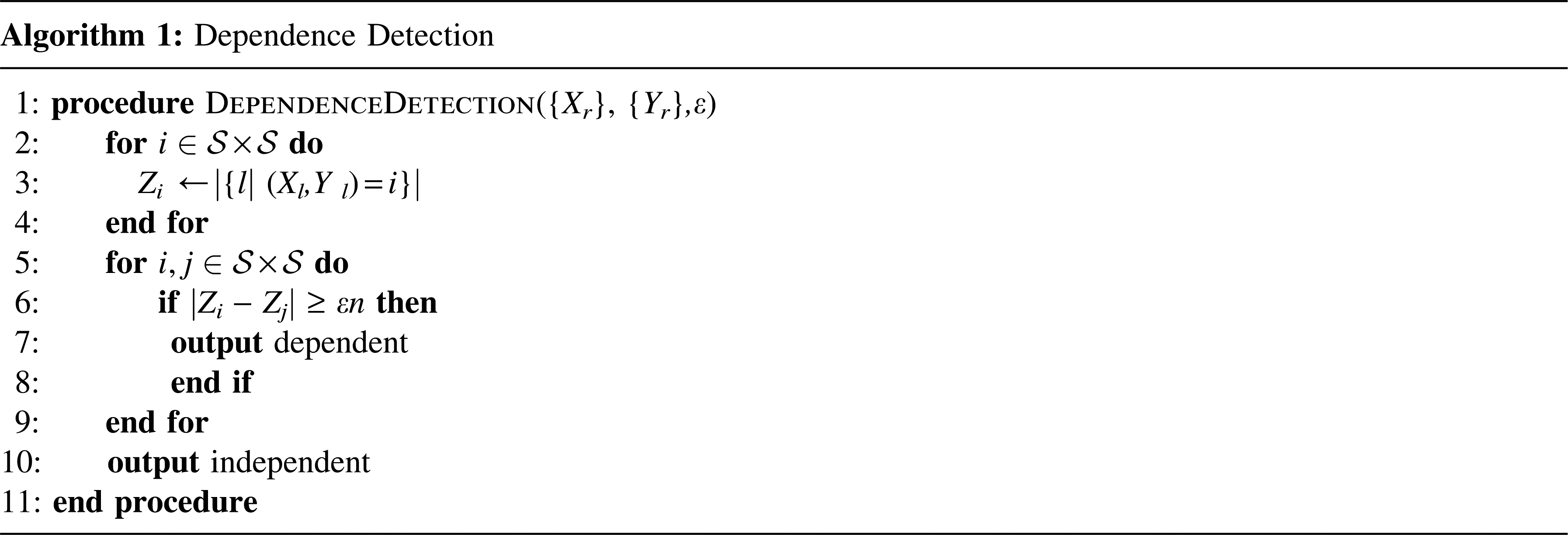
The input to our dependency testers are the values of the characters at the leaves of the phylogeny. Our tester is extremely simple: For each ordered pair of states, we count the number of leaves that have that pair. If there is a “large discrepancy” in this number, the characters are dependent.

OPEN IN VIEWER

Note that we have used a single index i to denote a pair of states. The {X_l} and {Y_l} are the leaf states of the two characters. We now briefly outline the analysis and the challenges involved.

We prove a concentration bound for the overall distribution of state pairs at the leaves. For all ordered pairs i, we need that the number of leaves Z_i that have the state i, is concentrated around its mean. This is not trivial since Z_i is a sum of indicator random variables that are not independent, because in a tree Markov random field, even the state of one character at “nearby” leaves are highly correlated. We obtain concentration by upper-bounding the second moment (Theorem 4.1), which is done via a coarse but sufficiently good upper bound on the variance (Lemma 4.3). We also show that when the characters are independent, we expect each joint state to be almost equally likely (Lemma 5.2). Since the norms of the transition matrices are bounded away from 1, we expect rapid mixing and the leaf state to be close to stationary distribution, which by the assumption of double-stochasticity is uniform.

In the case of dependent characters, we show that a large discrepancy indeed occurs (in expectation) for at least one pair of states (Lemma 5.3). This is nontrivial since different edges have different transition matrices, and the effect of one matrix's deviation may cancel the effect of its predecessors. Indeed, in the PSD model, we show that this can happen even when λ₂ ≥ 0.832 (Lemma 5.7). However, if all matrices share the same eigenbasis, then such a “bad case” cannot occur (Lemma 5.4), and so the shared eigenbase model doesn't need any further assumptions. In the doubly stochastic model, an upper bound of 0.5 suffices (Lemma 5.8) to detect dependency. For the PSD model, an upper bound λ₂ ≤ 0.797 suffices, and this is more subtle to show. To do so, we prove a lower bound on a quantity v^⊤Av where A is a product of k PSD matrices (and therefore, not necessarily PSD), and v is a vector perpendicular to the all ones vector. We show (Lemma 5.6) that this quantity is at least \documentclass{aastex}\usepackage{amsbsy}\usepackage{amsfonts}\usepackage{amssymb}\usepackage{bm}\usepackage{mathrsfs}\usepackage{pifont}\usepackage{stmaryrd}\usepackage{textcomp}\usepackage{portland, xspace}\usepackage{amsmath, amsxtra}\pagestyle{empty}\DeclareMathSizes{10}{9}{7}{6}\begin{document} $$- ( \lambda \cos ( \pi / k + 1 ) ) ^k \parallel v \parallel _2^2$$ \end{document} ; this result may be of independent interest. We leave open the question of finding the exact value in [0.797, 0.832] at which dependence can be detected in the PSD model. Finally, in Theorem 6.1, we show that in the directional-dependence model, we can detect dependence when λ* is bounded by a function of δ, β.

4. Bounding the Variance

Fix an \documentclass{aastex}\usepackage{amsbsy}\usepackage{amsfonts}\usepackage{amssymb}\usepackage{bm}\usepackage{mathrsfs}\usepackage{pifont}\usepackage{stmaryrd}\usepackage{textcomp}\usepackage{portland, xspace}\usepackage{amsmath, amsxtra}\pagestyle{empty}\DeclareMathSizes{10}{9}{7}{6}\begin{document} $$i \in { \cal P} = { \cal S} \times { \cal S}$$ \end{document} . Let Z be the random variable counting the number of leaves of T in state i. For a random variable X, let E[X] denote its expectation and V(X) its variance. Recall λ < 1 is an upper bound on the norm of any of the transition matrices P_e on the edges e. In this section, we prove the following theorem.

Theorem 4.1. Given any n leaf trivalent tree T, V(Z) = O(n^{2–2 log₂(1/λ)}).

For any vertex v in T, let Z_v be the number of leaves in the subtree of T rooted at v in state in i; so Z = Z_root. Let L_v denote the leaves in the subtree rooted at v. For a leaf ℓ ∈ L_v, let dist(v,ℓ) denote the number of edges on the path from v to ℓ in the tree. Define \documentclass{aastex}\usepackage{amsbsy}\usepackage{amsfonts}\usepackage{amssymb}\usepackage{bm}\usepackage{mathrsfs}\usepackage{pifont}\usepackage{stmaryrd}\usepackage{textcomp}\usepackage{portland, xspace}\usepackage{amsmath, amsxtra}\pagestyle{empty}\DeclareMathSizes{10}{9}{7}{6}\begin{document} \begin{align*}\Lambda ( v ) \ 2 \sum\limits_{ \ell \in L_u} \lambda^{\rm dist} ( v , \ell ) \tag{1}\end{align*} \end{document}

The following claim bounds Λ(v) at any vertex.

Proposition 4.2. For any vertex u with n leaves in its subtree, Λ(u) ≤ O(n^1–η) where η = log₂(1/λ).

Proof. Note that \documentclass{aastex}\usepackage{amsbsy}\usepackage{amsfonts}\usepackage{amssymb}\usepackage{bm}\usepackage{mathrsfs}\usepackage{pifont}\usepackage{stmaryrd}\usepackage{textcomp}\usepackage{portland, xspace}\usepackage{amsmath, amsxtra}\pagestyle{empty}\DeclareMathSizes{10}{9}{7}{6}\begin{document} $$\Lambda ( u ) = 2 \sum \nolimits_{i \ge 1} \mid L_i \mid \lambda^i$$ \end{document} where L_i is the set of leaves at a distance i from u. Since λ < 1, an n leaf tree that maximizes Λ(u) will make the tree as balanced in height as possible. (This can be proved by a “swapping” argument similar to the proof of optimality of Huffman trees.) In particular, the maximizing tree has all leaves at distance \documentclass{aastex}\usepackage{amsbsy}\usepackage{amsfonts}\usepackage{amssymb}\usepackage{bm}\usepackage{mathrsfs}\usepackage{pifont}\usepackage{stmaryrd}\usepackage{textcomp}\usepackage{portland, xspace}\usepackage{amsmath, amsxtra}\pagestyle{empty}\DeclareMathSizes{10}{9}{7}{6}\begin{document} $$\lfloor \log \ n \rfloor$$ \end{document} or \documentclass{aastex}\usepackage{amsbsy}\usepackage{amsfonts}\usepackage{amssymb}\usepackage{bm}\usepackage{mathrsfs}\usepackage{pifont}\usepackage{stmaryrd}\usepackage{textcomp}\usepackage{portland, xspace}\usepackage{amsmath, amsxtra}\pagestyle{empty}\DeclareMathSizes{10}{9}{7}{6}\begin{document} $$\lfloor \log \ n \rfloor + 1$$ \end{document} . Therefore, \documentclass{aastex}\usepackage{amsbsy}\usepackage{amsfonts}\usepackage{amssymb}\usepackage{bm}\usepackage{mathrsfs}\usepackage{pifont}\usepackage{stmaryrd}\usepackage{textcomp}\usepackage{portland, xspace}\usepackage{amsmath, amsxtra}\pagestyle{empty}\DeclareMathSizes{10}{9}{7}{6}\begin{document} $$\Lambda ( v ) \le \frac { 2 } { \lambda } \cdot n \lambda^ { \log n } = \frac { 2 } { \lambda } \cdot n^ { 1 - \log ( 1 / \lambda ) } $$ \end{document} .    ■

The next lemma bounds the variance in terms of the Λ's. We will use the lemma to prove the theorem.

Lemma 4.3.  \documentclass{aastex}\usepackage{amsbsy}\usepackage{amsfonts}\usepackage{amssymb}\usepackage{bm}\usepackage{mathrsfs}\usepackage{pifont}\usepackage{stmaryrd}\usepackage{textcomp}\usepackage{portland, xspace}\usepackage{amsmath, amsxtra}\pagestyle{empty}\DeclareMathSizes{10}{9}{7}{6}\begin{document} $$ { \bf V } ( Z ) \le \frac { 1 } { 2 } \sum \nolimits_ { v \in V ( T ) / { \rm root } } ( \Lambda ( v ) ) ^2$$ \end{document} .

Proof. For a vertex v and two states \documentclass{aastex}\usepackage{amsbsy}\usepackage{amsfonts}\usepackage{amssymb}\usepackage{bm}\usepackage{mathrsfs}\usepackage{pifont}\usepackage{stmaryrd}\usepackage{textcomp}\usepackage{portland, xspace}\usepackage{amsmath, amsxtra}\pagestyle{empty}\DeclareMathSizes{10}{9}{7}{6}\begin{document} $$j , k \in {\cal P}$$ \end{document} , define \documentclass{aastex}\usepackage{amsbsy}\usepackage{amsfonts}\usepackage{amssymb}\usepackage{bm}\usepackage{mathrsfs}\usepackage{pifont}\usepackage{stmaryrd}\usepackage{textcomp}\usepackage{portland, xspace}\usepackage{amsmath, amsxtra}\pagestyle{empty}\DeclareMathSizes{10}{9}{7}{6}\begin{document} \begin{align*}\Delta_v ( j , k ) \Delta \mid { \bf {E}} \left[ Z_v \mid X_v = j \right] - { \bf {E}} \left[ Z_v \mid X_v = k \right] \mid \tag{2}\end{align*} \end{document}

The following claim relates Δ _v with Λ(v).

Claim 4.4. For any vertex v, and for any two states \documentclass{aastex}\usepackage{amsbsy}\usepackage{amsfonts}\usepackage{amssymb}\usepackage{bm}\usepackage{mathrsfs}\usepackage{pifont}\usepackage{stmaryrd}\usepackage{textcomp}\usepackage{portland, xspace}\usepackage{amsmath, amsxtra}\pagestyle{empty}\DeclareMathSizes{10}{9}{7}{6}\begin{document} $$j , k \in {\cal P}$$ \end{document} , we have Δ _v (j,k) ≤ Λ(v).

Proof. Fix a vertex v and a leaf ℓ ∈ L_v. Let e₁, e₂, … , e_dist(v,ℓ) be the edges on the path from v to ℓ. Let P denote the matrix \documentclass{aastex}\usepackage{amsbsy}\usepackage{amsfonts}\usepackage{amssymb}\usepackage{bm}\usepackage{mathrsfs}\usepackage{pifont}\usepackage{stmaryrd}\usepackage{textcomp}\usepackage{portland, xspace}\usepackage{amsmath, amsxtra}\pagestyle{empty}\DeclareMathSizes{10}{9}{7}{6}\begin{document} $$P_{e_1} \cdot P_{e_2} \cdots P_{e_{{ \rm dist} ( v , \ell ) }}$$ \end{document} ; this is the transition matrix from v to leaf ℓ. In particular, P is row-stochastic (row entries add up to 1). We use the following simple fact about row stochastic matrices; another proof of this can be found in Lemma 4.12 in Levin et al., (2009).

Claim 4.5. For any two row stochastic matrices P₁ and P₂, we have ||P₁P₂||≤||P₁||·||P₂||.

Proof. Let x be the vector with ||x||₁ = 1 and x⊤1 = 0 such that ||P₁P₂|| = ||x^⊤P₁P₂||₁. Note that y^⊤ = x^⊤P₁ also satisfies y^⊤1 = 0 since P₁ is row stochastic. Therefore, ||y^⊤P₂||₁ ≤ ||y||₁ · ||P₂||. Also by definition, ||y||₁ = ||x^⊤P₁||₁ ≤ ||P₁||.    ■

This claim implies that ||P|| is at most λ^dist(v,ℓ). In particular, this shows that for any vertex v, for any leaf ℓ ∈ L_v at a distance dist(v,ℓ), and for any states \documentclass{aastex}\usepackage{amsbsy}\usepackage{amsfonts}\usepackage{amssymb}\usepackage{bm}\usepackage{mathrsfs}\usepackage{pifont}\usepackage{stmaryrd}\usepackage{textcomp}\usepackage{portland, xspace}\usepackage{amsmath, amsxtra}\pagestyle{empty}\DeclareMathSizes{10}{9}{7}{6}\begin{document} $$j , k \in {\cal S}$$ \end{document} , we have |P[X_ℓ = i|X_v = j] – P[X_ℓ = i|X_v = k]| ≤ ||x^T P||₁ ≤ 2λ^dist(v,ℓ), where x is the vector with x_j = 1, x_k = –1, and x_s = 0 otherwise. The claim follows by noting \documentclass{aastex}\usepackage{amsbsy}\usepackage{amsfonts}\usepackage{amssymb}\usepackage{bm}\usepackage{mathrsfs}\usepackage{pifont}\usepackage{stmaryrd}\usepackage{textcomp}\usepackage{portland, xspace}\usepackage{amsmath, amsxtra}\pagestyle{empty}\DeclareMathSizes{10}{9}{7}{6}\begin{document} \begin{align*} \Delta_v ( j , k ) & = \mid \sum \limits_{ \ell \in L_v} ( { \bf {P}} \left[ X_{ \ell} = i \mid X_v = j \right] - { \bf {P}} \left[ X_{ \ell} = i \mid X_v = k \right] ) \mid \\ & \leq \sum \limits_{ \ell \in L_v} \mid { \bf {P}} \left[ X_{ \ell} = i \mid X_v = j \right] - { \bf {P}} \left[ X_{ \ell} = i \mid X_v = k \right] \mid \leq 2 \sum \limits_{ \ell \in L_v} \lambda^{\rm dist} ( v , \ell ) \end{align*} \end{document}    ▪

Now we can finish the proof of Lemma 4.3. Fix any vertex u. Recall that T_u denotes the subtree of T rooted at u, and Z_u is the number of leaves in L_u in state i. We now show using induction on the height of T that for any state \documentclass{aastex}\usepackage{amsbsy}\usepackage{amsfonts}\usepackage{amssymb}\usepackage{bm}\usepackage{mathrsfs}\usepackage{pifont}\usepackage{stmaryrd}\usepackage{textcomp}\usepackage{portland, xspace}\usepackage{amsmath, amsxtra}\pagestyle{empty}\DeclareMathSizes{10}{9}{7}{6}\begin{document} $$j \in { { \cal P } } , { \bf V } ( Z_u \mid X_u = j ) \leq \frac { 1 } { 2 } \sum \nolimits_ { v \in V ( T_u ) \backslash u } \Lambda^2 ( v )$$ \end{document} . This proves the lemma with u as the root, and summing over all the conditional events.

Note that the claim is vacuously true when u is a leaf since both LHS and RHS are 0. Let u have children v₁, … , v_q (if the tree is binary, q = 2, but this lemma holds for any tree). Assume we have proved the inductive claim for the v_i's. Note that conditioned on X_u, the random variables Z_v1, Z_v2, …  are independent, since they count over leaves on disjoint subtrees. Therefore, for any \documentclass{aastex}\usepackage{amsbsy}\usepackage{amsfonts}\usepackage{amssymb}\usepackage{bm}\usepackage{mathrsfs}\usepackage{pifont}\usepackage{stmaryrd}\usepackage{textcomp}\usepackage{portland, xspace}\usepackage{amsmath, amsxtra}\pagestyle{empty}\DeclareMathSizes{10}{9}{7}{6}\begin{document} $$j \in { {\cal P}} , { \bf V} ( Z_u \mid X_u = j ) = \sum \nolimits^q_{i = 1}{ \bf {V}} \left( Z_{v_i} \mid X_u = j \right)$$ \end{document} .

We now show that for any parent–child pair e = (u,v_i), and any state \documentclass{aastex}\usepackage{amsbsy}\usepackage{amsfonts}\usepackage{amssymb}\usepackage{bm}\usepackage{mathrsfs}\usepackage{pifont}\usepackage{stmaryrd}\usepackage{textcomp}\usepackage{portland, xspace}\usepackage{amsmath, amsxtra}\pagestyle{empty}\DeclareMathSizes{10}{9}{7}{6}\begin{document} $$j \in {\cal P}$$ \end{document} , we have \documentclass{aastex}\usepackage{amsbsy}\usepackage{amsfonts}\usepackage{amssymb}\usepackage{bm}\usepackage{mathrsfs}\usepackage{pifont}\usepackage{stmaryrd}\usepackage{textcomp}\usepackage{portland, xspace}\usepackage{amsmath, amsxtra}\pagestyle{empty}\DeclareMathSizes{10}{9}{7}{6}\begin{document} \begin{align*} { \bf { V } } ( Z_ { v_i } \mid X_u = j ) = \sum \limits_ { k \in { \cal P } } P_ { jk } { \bf { V } } ( Z_ { v_i } \mid X_v = k ) + \frac { 1 } { 2 } \sum \limits_ { k \neq k^ \prime \in { \cal P } } P_ { jk } P_ { jk^ \prime } \Delta^2_ { v_i } ( k , k^ { \prime } ) \tag { 3 } \end{align*} \end{document}

where P_jk = P[X_vi = k|X_u = j] = P_e(j, k). Equation (3) suffices to complete the proof. By induction, the first summand in the RHS is at most \documentclass{aastex}\usepackage{amsbsy}\usepackage{amsfonts}\usepackage{amssymb}\usepackage{bm}\usepackage{mathrsfs}\usepackage{pifont}\usepackage{stmaryrd}\usepackage{textcomp}\usepackage{portland, xspace}\usepackage{amsmath, amsxtra}\pagestyle{empty}\DeclareMathSizes{10}{9}{7}{6}\begin{document} $$ \frac { 1 } { 2 } \sum \nolimits_ { w \in T_ { v_i } \backslash v_i } \Lambda^2 ( w )$$ \end{document} . From Claim 4.4, we have Δ _vi (k,k′) ≤ Λ(v_i) and \documentclass{aastex}\usepackage{amsbsy}\usepackage{amsfonts}\usepackage{amssymb}\usepackage{bm}\usepackage{mathrsfs}\usepackage{pifont}\usepackage{stmaryrd}\usepackage{textcomp}\usepackage{portland, xspace}\usepackage{amsmath, amsxtra}\pagestyle{empty}\DeclareMathSizes{10}{9}{7}{6}\begin{document} $$\sum \nolimits_{k \neq k{ \prime}} P_{jk} P_{jk^{ \prime}} \leq \left( \sum \nolimits_{k \in { \cal P}} P_{jk} \right) ^2 = 1$$ \end{document} , thereby giving that the second summand in the RHS of Equation (3) is at most \documentclass{aastex}\usepackage{amsbsy}\usepackage{amsfonts}\usepackage{amssymb}\usepackage{bm}\usepackage{mathrsfs}\usepackage{pifont}\usepackage{stmaryrd}\usepackage{textcomp}\usepackage{portland, xspace}\usepackage{amsmath, amsxtra}\pagestyle{empty}\DeclareMathSizes{10}{9}{7}{6}\begin{document} $$ \frac { 1 } { 2 } \Lambda^2 ( v_i )$$ \end{document} . Together, we get \documentclass{aastex}\usepackage{amsbsy}\usepackage{amsfonts}\usepackage{amssymb}\usepackage{bm}\usepackage{mathrsfs}\usepackage{pifont}\usepackage{stmaryrd}\usepackage{textcomp}\usepackage{portland, xspace}\usepackage{amsmath, amsxtra}\pagestyle{empty}\DeclareMathSizes{10}{9}{7}{6}\begin{document} $$ { \bf { V } } ( Z_ { v_i } \mid X_u = j ) \leq \frac { 1 } { 2 } \sum \nolimits_ { w \in T_ { v_i } } \Lambda^2 ( w )$$ \end{document} , and by adding over all v _i , 1 ≤ i ≤ q, we complete the proof of Lemma 4.3.

Proof of theorem 4.1. Let \documentclass{aastex}\usepackage{amsbsy}\usepackage{amsfonts}\usepackage{amssymb}\usepackage{bm}\usepackage{mathrsfs}\usepackage{pifont}\usepackage{stmaryrd}\usepackage{textcomp}\usepackage{portland, xspace}\usepackage{amsmath, amsxtra}\pagestyle{empty}\DeclareMathSizes{10}{9}{7}{6}\begin{document} $$\nu ( n )$$ \end{document} be a function that denotes the maximum value of \documentclass{aastex}\usepackage{amsbsy}\usepackage{amsfonts}\usepackage{amssymb}\usepackage{bm}\usepackage{mathrsfs}\usepackage{pifont}\usepackage{stmaryrd}\usepackage{textcomp}\usepackage{portland, xspace}\usepackage{amsmath, amsxtra}\pagestyle{empty}\DeclareMathSizes{10}{9}{7}{6}\begin{document} $$\sum \nolimits_{v \in V ( T ) \backslash r} \Lambda^2 ( v )$$ \end{document} over all n-leaf binary trees. By Lemma 4.3, we want a subquadratic upperbound on \documentclass{aastex}\usepackage{amsbsy}\usepackage{amsfonts}\usepackage{amssymb}\usepackage{bm}\usepackage{mathrsfs}\usepackage{pifont}\usepackage{stmaryrd}\usepackage{textcomp}\usepackage{portland, xspace}\usepackage{amsmath, amsxtra}\pagestyle{empty}\DeclareMathSizes{10}{9}{7}{6}\begin{document} $$\nu ( n )$$ \end{document} . Let u be the centroid of T. That is, n/3 ≤ |L_u| ≤ 2n/3. It is easy to see this is well defined. Let T_u denote the subtree of T rooted at u, and let T′ _u denote the subtree of T with all descendants of u deleted. Note that both T_u and T′ _u are binary trees, and have ρn and (1 – ρ)n leaves for ρ ∈ [1/3, 2/3]. By definition, \documentclass{aastex}\usepackage{amsbsy}\usepackage{amsfonts}\usepackage{amssymb}\usepackage{bm}\usepackage{mathrsfs}\usepackage{pifont}\usepackage{stmaryrd}\usepackage{textcomp}\usepackage{portland, xspace}\usepackage{amsmath, amsxtra}\pagestyle{empty}\DeclareMathSizes{10}{9}{7}{6}\begin{document} $$\sum \nolimits_{v \in V ( Tu ) \backslash u} \Lambda^2 ( v ) \leq \nu ( \rho n )$$ \end{document} and \documentclass{aastex}\usepackage{amsbsy}\usepackage{amsfonts}\usepackage{amssymb}\usepackage{bm}\usepackage{mathrsfs}\usepackage{pifont}\usepackage{stmaryrd}\usepackage{textcomp}\usepackage{portland, xspace}\usepackage{amsmath, amsxtra}\pagestyle{empty}\DeclareMathSizes{10}{9}{7}{6}\begin{document} $$\sum \nolimits_{v \in V ( T^{ \prime}_u ) \backslash r} \Lambda^2 ( v ) \leq \nu ( ( 1 - \rho ) n )$$ \end{document} .

Suppose u = u₀, u₁, … , u_r = r is the unique path from u to r in T. Note that the Λ(v)'s in tree T′ _u are the same as in tree T for all vertices except the u_i's. For each u_i, Λ(u_i) in the tree T is that in T′ _u plus λⁱ · Λ(u). Thus, we have \documentclass{aastex}\usepackage{amsbsy}\usepackage{amsfonts}\usepackage{amssymb}\usepackage{bm}\usepackage{mathrsfs}\usepackage{pifont}\usepackage{stmaryrd}\usepackage{textcomp}\usepackage{portland, xspace}\usepackage{amsmath, amsxtra}\pagestyle{empty}\DeclareMathSizes{10}{9}{7}{6}\begin{document} \begin{align*} \sum \limits_{v \in V ( T ) \backslash r} \Lambda^2 ( v ) & \leq \, { \nu ( \rho n ) + \nu ( ( 1 - \rho ) n ) + \mathop \sum \limits^r_{i = 0} \left( ( \Lambda ( u_i ) + 2 \lambda^i \Lambda ( u ) ) ^2 - \Lambda^2 ( u_i ) \right) } \\ & = \,\nu ( \rho n ) + \nu ( ( 1 - \rho ) n ) + 4 \Lambda ( u ) \mathop \sum \limits^r_{i = 0} \lambda^i \Lambda ( u_i ) + 4 \Lambda^2 ( u ) \mathop \sum \limits^r_{i = 0} \lambda^{2i}\end{align*} \end{document}

From Proposition 4.2, we can bound Λ(u_i) by O(n^1–η) for i = 0, … , r. So we get the following recurrence for \documentclass{aastex}\usepackage{amsbsy}\usepackage{amsfonts}\usepackage{amssymb}\usepackage{bm}\usepackage{mathrsfs}\usepackage{pifont}\usepackage{stmaryrd}\usepackage{textcomp}\usepackage{portland, xspace}\usepackage{amsmath, amsxtra}\pagestyle{empty}\DeclareMathSizes{10}{9}{7}{6}\begin{document} $$\nu ( n ) \ \nu ( n ) \leq \nu ( \rho n ) + \nu ( ( 1 - \rho ) n ) + O ( n^{2 - 2 \eta} )$$ \end{document} , which evaluates to \documentclass{aastex}\usepackage{amsbsy}\usepackage{amsfonts}\usepackage{amssymb}\usepackage{bm}\usepackage{mathrsfs}\usepackage{pifont}\usepackage{stmaryrd}\usepackage{textcomp}\usepackage{portland, xspace}\usepackage{amsmath, amsxtra}\pagestyle{empty}\DeclareMathSizes{10}{9}{7}{6}\begin{document} $$\nu ( n ) = O ( n^{2 - 2 \eta} )$$ \end{document} .    ■

5. Analysis of the Tester in Uniform Rank-1 Model

Let μ₀ be the state at the root. Let μ be the uniform distribution over the s² states. Let r₀ = μ₀ – μ be the error vector at the root. Recall P_e is the transition matrix of the joint random variable (X, Y ) at edge e. We write P_e = Q_e + D where \documentclass{aastex}\usepackage{amsbsy}\usepackage{amsfonts}\usepackage{amssymb}\usepackage{bm}\usepackage{mathrsfs}\usepackage{pifont}\usepackage{stmaryrd}\usepackage{textcomp}\usepackage{portland, xspace}\usepackage{amsmath, amsxtra}\pagestyle{empty}\DeclareMathSizes{10}{9}{7}{6}\begin{document} $$Q_e = M_e \otimes N_e$$ \end{document} and D is the zero-matrix if the characters are independent, and D = 1d^⊤ in case the characters are dependent.

Our goal in this section is to establish the following theorem, ⁴ asserting the correctness of the tester for the uniform rank-1 model.

Theorem 5.1. Under each of the following evolutionary models, under the listed assumptions on the norm on the transition matrices, algorithm Dependence Detection is correct with 1 – 1/poly(n) probability.

Shared eigenbasis. No extra assumption on Q_e is needed.

PSD. If λ₂(Q_e) ≤ 0.797.

Doubly stochastic. If λ₂(Q_e) ≤ 0.5.

For a leaf ℓ, let μ_ℓ be the distribution at the leaf, and r_ℓ = μ_ℓ – μ be the error vector at the leaf. Let (e₁, e₂, … , e_dist(ℓ)) be the path from the root to the leaf ℓ. Then, if the characters are independent, we get \documentclass{aastex}\usepackage{amsbsy}\usepackage{amsfonts}\usepackage{amssymb}\usepackage{bm}\usepackage{mathrsfs}\usepackage{pifont}\usepackage{stmaryrd}\usepackage{textcomp}\usepackage{portland, xspace}\usepackage{amsmath, amsxtra}\pagestyle{empty}\DeclareMathSizes{10}{9}{7}{6}\begin{document} \begin{align*}r^{\top}_{ \ell} = r_0^{\top} \left( \prod^{\rm dist ( \ell ) }_{k = 1} Q_{e_k} \right) \tag{4}\end{align*} \end{document}

and if the characters are dependent, we get \documentclass{aastex}\usepackage{amsbsy}\usepackage{amsfonts}\usepackage{amssymb}\usepackage{bm}\usepackage{mathrsfs}\usepackage{pifont}\usepackage{stmaryrd}\usepackage{textcomp}\usepackage{portland, xspace}\usepackage{amsmath, amsxtra}\pagestyle{empty}\DeclareMathSizes{10}{9}{7}{6}\begin{document} \begin{align*}r^{\top}_{ \ell} = d^{\top} + \mathop \sum \limits_{i = 1}^{\rm dist ( \ell ) } d^{\top} \left( \prod_{k = i + 1}^{\rm dist ( \ell ) - 1} Q_{e_k} \right) + r_0^{\top} \left( \prod_{k = 1}^{\rm dist ( \ell )} Q_{e_k} \right) \tag{5}\end{align*} \end{document}

We first prove a lemma to show that when the character pair evolves independently, the distribution of state pairs at the leaves is close to uniform.

Lemma 5.2. If the characters are independent, then for all \documentclass{aastex}\usepackage{amsbsy}\usepackage{amsfonts}\usepackage{amssymb}\usepackage{bm}\usepackage{mathrsfs}\usepackage{pifont}\usepackage{stmaryrd}\usepackage{textcomp}\usepackage{portland, xspace}\usepackage{amsmath, amsxtra}\pagestyle{empty}\DeclareMathSizes{10}{9}{7}{6}\begin{document} $$i \in {\cal P}$$ \end{document} , we have |E[Z_i] − n/s²| ≤ O(n^1−β) for some constant β depending on λ, the upper bound on the norms of all the transition matrices.

Proof. By our assumption, ||Q_ei|| ≤ λ for all i. Substituting in Equation (4), and using Fact 4.5, we get ||r_ℓ||₁ ≤ λ^dist(ℓ)||r ₀||₁ ≤ 2λ^dist(ℓ) since ||r₀||₁ ≤ ||μ||₁ + ||μ₀||₁ = 2. In turn, this implies |〈r_ℓ,e_i〈| ≤ 2λ^dist(ℓ). Note for any i, we have E[Z_i] = ∑ _ℓ 〈μ_ℓ,e_i〉 = n/s² + ∑ _ℓ 〈r_ℓ,e_i〉 ≤ n/s² + Λ(root), and the lemma follows from Proposition 4.2.    ■

Next, we prove a contrasting lemma for the dependent case, depending on the model of evolution. In each case, we show that there is a deviation from the uniform in the distribution at the leaves. In particular, we exhibit \documentclass{aastex}\usepackage{amsbsy}\usepackage{amsfonts}\usepackage{amssymb}\usepackage{bm}\usepackage{mathrsfs}\usepackage{pifont}\usepackage{stmaryrd}\usepackage{textcomp}\usepackage{portland, xspace}\usepackage{amsmath, amsxtra}\pagestyle{empty}\DeclareMathSizes{10}{9}{7}{6}\begin{document} $$r^{*} \in {\mathbb R}^{s^2}$$ \end{document} , whose coordinates sum up to zero with each entry in [−1, +1] such that there is some ɛ > 0 satisfying: \documentclass{aastex}\usepackage{amsbsy}\usepackage{amsfonts}\usepackage{amssymb}\usepackage{bm}\usepackage{mathrsfs}\usepackage{pifont}\usepackage{stmaryrd}\usepackage{textcomp}\usepackage{portland, xspace}\usepackage{amsmath, amsxtra}\pagestyle{empty}\DeclareMathSizes{10}{9}{7}{6}\begin{document} \begin{align*}{ \rm For \ all} \ \ell , { \rm we \ have} \ \ \langle r_{ \ell , } r^{*} \rangle \geq \varepsilon. \tag{{ \rm Deviation}}\end{align*} \end{document}

We prove the following lemma, under the assumption that this equation is satisfied. In later subsections, we demonstrate, r* in every model of evolution.

Lemma 5.3. If under a model of evolution we obtain an r* and ɛ satisfying (Deviation), then there exists \documentclass{aastex}\usepackage{amsbsy}\usepackage{amsfonts}\usepackage{amssymb}\usepackage{bm}\usepackage{mathrsfs}\usepackage{pifont}\usepackage{stmaryrd}\usepackage{textcomp}\usepackage{portland, xspace}\usepackage{amsmath, amsxtra}\pagestyle{empty}\DeclareMathSizes{10}{9}{7}{6}\begin{document} $$i , j \in {\cal P}$$ \end{document} such that |E[Z_i] – E[Z_j]| ≥ ɛn where ɛ is a constant depending on δ and s.

Proof. Let \documentclass{aastex}\usepackage{amsbsy}\usepackage{amsfonts}\usepackage{amssymb}\usepackage{bm}\usepackage{mathrsfs}\usepackage{pifont}\usepackage{stmaryrd}\usepackage{textcomp}\usepackage{portland, xspace}\usepackage{amsmath, amsxtra}\pagestyle{empty}\DeclareMathSizes{10}{9}{7}{6}\begin{document} $$\bar { \mu } \ : = \frac { 1 } { n } \sum \nolimits_ { \ell } \mu_ { \ell } $$ \end{document} . Observe that 〈 \documentclass{aastex}\usepackage{amsbsy}\usepackage{amsfonts}\usepackage{amssymb}\usepackage{bm}\usepackage{mathrsfs}\usepackage{pifont}\usepackage{stmaryrd}\usepackage{textcomp}\usepackage{portland, xspace}\usepackage{amsmath, amsxtra}\pagestyle{empty}\DeclareMathSizes{10}{9}{7}{6}\begin{document} $$\bar { \mu}$$ \end{document} , r*〉 ≥ ɛ as well. Since r* is a convex combination of vectors of the form {e_i – e_j}, where e_i is the indicator vector for pair i, we get there exists (i,j) such that \documentclass{aastex}\usepackage{amsbsy}\usepackage{amsfonts}\usepackage{amssymb}\usepackage{bm}\usepackage{mathrsfs}\usepackage{pifont}\usepackage{stmaryrd}\usepackage{textcomp}\usepackage{portland, xspace}\usepackage{amsmath, amsxtra}\pagestyle{empty}\DeclareMathSizes{10}{9}{7}{6}\begin{document} $$\langle \bar { \mu} , ( e_i - e_j ) \rangle \geq \varepsilon$$ \end{document} . But \documentclass{aastex}\usepackage{amsbsy}\usepackage{amsfonts}\usepackage{amssymb}\usepackage{bm}\usepackage{mathrsfs}\usepackage{pifont}\usepackage{stmaryrd}\usepackage{textcomp}\usepackage{portland, xspace}\usepackage{amsmath, amsxtra}\pagestyle{empty}\DeclareMathSizes{10}{9}{7}{6}\begin{document} $$\langle \bar { \mu} , e_i \rangle$$ \end{document} is precisely E[Z_i]/n since 〈μ_ℓ,e_i〉 indicates the probability leaf ℓ is in state i. Therefore, (Deviation) implies that there exists a pair i and j such that E[Z_i] – E[Z_j] ≥ ɛn.    ■

Proof of Theorem 5.1. These follow from Lemma 5.2 and Lemma 5.3 [with appropriate use of Eq. (Deviation)], using Lemmas 5.4, 5.5, and Lemma 5.8 given below; Theorem 4.1; and Chebyshev's inequality.    ■

6. Directional-Drift Dependence Model

Here, we generalize the error model, in the PSD evolution model, using the directional-drift dependence model that we now describe. We recall that PSD model generalizes the shared eigenbases model, which in turn generalizes all stochastic models studied in the literature. In this model, there is a fixed direction d*, such that every row of each error matrix has the following properties: (1) ∥d^⊤∥ ≤ δ/β, and (2) 〈d,d*〉 ≥ δ for a significant δ and a constant β.

Theorem 6.1. In the PSD evolutionary model with the directional-drift dependence model above, if all transition matrices have norm bounded by \documentclass{aastex}\usepackage{amsbsy}\usepackage{amsfonts}\usepackage{amssymb}\usepackage{bm}\usepackage{mathrsfs}\usepackage{pifont}\usepackage{stmaryrd}\usepackage{textcomp}\usepackage{portland, xspace}\usepackage{amsmath, amsxtra}\pagestyle{empty}\DeclareMathSizes{10}{9}{7}{6}\begin{document} $$\lambda^ { * } ( \beta ) = \frac { \beta } { \frac { 1 } { 2 } + \beta } $$ \end{document} , then dependence detection is correct.

This theorem will again follow from Lemmas 5.3 and 5.2, through the use of Equation (Deviation), with r* = d* and ɛ(β,λ).

Let us first examine now what happens in one step, when we start with a vector \documentclass{aastex}\usepackage{amsbsy}\usepackage{amsfonts}\usepackage{amssymb}\usepackage{bm}\usepackage{mathrsfs}\usepackage{pifont}\usepackage{stmaryrd}\usepackage{textcomp}\usepackage{portland, xspace}\usepackage{amsmath, amsxtra}\pagestyle{empty}\DeclareMathSizes{10}{9}{7}{6}\begin{document} $$\vec{u} + \vec{r}$$ \end{document} and apply the transform P_e = Q_e + D_e, \documentclass{aastex}\usepackage{amsbsy}\usepackage{amsfonts}\usepackage{amssymb}\usepackage{bm}\usepackage{mathrsfs}\usepackage{pifont}\usepackage{stmaryrd}\usepackage{textcomp}\usepackage{portland, xspace}\usepackage{amsmath, amsxtra}\pagestyle{empty}\DeclareMathSizes{10}{9}{7}{6}\begin{document} \begin{align*}( \mu + r ) ^{\top} \mapsto \mu^{\top} + r^{\top} Q_e + ( \mu + r ) ^{\top} D_e\end{align*} \end{document}

When D_e = 1d^T, we see the last term is precisely d^⊤. Now, however, we get some vector d_e which has \documentclass{aastex}\usepackage{amsbsy}\usepackage{amsfonts}\usepackage{amssymb}\usepackage{bm}\usepackage{mathrsfs}\usepackage{pifont}\usepackage{stmaryrd}\usepackage{textcomp}\usepackage{portland, xspace}\usepackage{amsmath, amsxtra}\pagestyle{empty}\DeclareMathSizes{10}{9}{7}{6}\begin{document} $$\parallel \vec{d} \parallel_2 \leq \delta / \beta$$ \end{document} and \documentclass{aastex}\usepackage{amsbsy}\usepackage{amsfonts}\usepackage{amssymb}\usepackage{bm}\usepackage{mathrsfs}\usepackage{pifont}\usepackage{stmaryrd}\usepackage{textcomp}\usepackage{portland, xspace}\usepackage{amsmath, amsxtra}\pagestyle{empty}\DeclareMathSizes{10}{9}{7}{6}\begin{document} $$\langle \vec{d}_{e} , \vec{d}^{*} \rangle \geq \delta$$ \end{document} . We will use primarily the fact that this added vector has these properties. As before, we will view the transform in the error space, where the transform is \documentclass{aastex}\usepackage{amsbsy}\usepackage{amsfonts}\usepackage{amssymb}\usepackage{bm}\usepackage{mathrsfs}\usepackage{pifont}\usepackage{stmaryrd}\usepackage{textcomp}\usepackage{portland, xspace}\usepackage{amsmath, amsxtra}\pagestyle{empty}\DeclareMathSizes{10}{9}{7}{6}\begin{document} \begin{align*}r^{\top} \mapsto r^{\top} Q_e + d_e\end{align*} \end{document}

Our approach to show that the detection of dependence is possible here will be by induction. In particular, we will show that for each node other than the root, there is some x* = x*(β), such that if the distribution at the node v is μ + r_v, then 〈r_v,d*〉 ≥ x*δ. This is true for the direct children of the root, as the distribution is precisely μ + d_e, where e is the edge connecting to the root. By hypothesis, 〈d_e,d*〉 ≥ δ. This gives us the base case for induction.

Before we prove the general case, we will first observe that \documentclass{aastex}\usepackage{amsbsy}\usepackage{amsfonts}\usepackage{amssymb}\usepackage{bm}\usepackage{mathrsfs}\usepackage{pifont}\usepackage{stmaryrd}\usepackage{textcomp}\usepackage{portland, xspace}\usepackage{amsmath, amsxtra}\pagestyle{empty}\DeclareMathSizes{10}{9}{7}{6}\begin{document} $$\parallel r \parallel_2 \leq \frac { 1 } { 1 - \lambda^ { * } } \frac { \delta } { \beta } $$ \end{document} . This is clear since every transform Q_e reduces the length by a factor λ*, and then we add a vector of length at most δ/β. The length bound then is just a geometric series.

To prove the general case of the induction, we first show that it suffices to examine the problem in two dimensions. So suppose that we have a deviation r, which satisfies that 〈r, d*〉 ≥ x* for some constant x* to be determined later. We want to show that for any positive semi-definite Q with all eigenvalues at most λ* and any \documentclass{aastex}\usepackage{amsbsy}\usepackage{amsfonts}\usepackage{amssymb}\usepackage{bm}\usepackage{mathrsfs}\usepackage{pifont}\usepackage{stmaryrd}\usepackage{textcomp}\usepackage{portland, xspace}\usepackage{amsmath, amsxtra}\pagestyle{empty}\DeclareMathSizes{10}{9}{7}{6}\begin{document} $$\vec{d}$$ \end{document} satisfying the length and inner product requirements above, that 〈Q^⊤r + d, d*〉 ≥ x*.

It is clear that we only need to concern ourselves with the space of at most three dimensions spanned by d*, r, Q^⊤r, since the added d will add some fixed amount in the direction of d*. We are concerned with how negative 〈Q^⊤r, d*〉 can be. We know that for any direction z, if Q^⊤r is in the direction z, the largest length it can have is ∥r∥₂ cos θ where θ is the angle between z and r. Then in taking the inner product with d*, we gain another factor φ, where φ is the angle between z and r. So if Q^⊤r is not in the same plane as d* and r, then since cos is increasing in the range [0, π/2), we can replace z with z′, which is the projection of z into the plane of d* and r, then both θ and φ increase, and the resulting 〈Q^⊤r, d*〉 is more negative. Since we are concerned here with the worst case, it suffices to consider only when Q^⊤r lies in the plane of r and d*, thus reducing the induction step to two dimensions.

Now we prove the general step of the induction. We know that we can view this in two dimensions, so let us take d* to be the x-axis (recall that we defined it to be unit length, so we can do this without distorting lengths). Again, we are concerned with minimizing 〈Q^⊤r, d*〉. As we have seen, we can assume Q is a scaled projection. So if it is onto a vector z, which forms an angle θ with r and φ with the negative x-axis, then \documentclass{aastex}\usepackage{amsbsy}\usepackage{amsfonts}\usepackage{amssymb}\usepackage{bm}\usepackage{mathrsfs}\usepackage{pifont}\usepackage{stmaryrd}\usepackage{textcomp}\usepackage{portland, xspace}\usepackage{amsmath, amsxtra}\pagestyle{empty}\DeclareMathSizes{10}{9}{7}{6}\begin{document} \begin{align*}\langle Q^{\top} r , d^{*} \rangle \geq \lambda^{*} \parallel r \parallel_2 \cos ( \theta ) \cos ( \phi ) \geq \lambda^{*} \parallel r \parallel_2 \cos^2 ( \psi / 2 )\end{align*} \end{document}

where ψ is the angle between r and the negative x-axis. Let r = (x,y) now. Our inductive hypothesis is that x ≥ x*δ. We also have φ = tan ⁻¹(y/x). Standard trigonometric manipulations (and careful choice of sign) give us that \documentclass{aastex}\usepackage{amsbsy}\usepackage{amsfonts}\usepackage{amssymb}\usepackage{bm}\usepackage{mathrsfs}\usepackage{pifont}\usepackage{stmaryrd}\usepackage{textcomp}\usepackage{portland, xspace}\usepackage{amsmath, amsxtra}\pagestyle{empty}\DeclareMathSizes{10}{9}{7}{6}\begin{document} \begin{align*}\parallel r \parallel_2 \cos^2 ( \psi / 2 ) \geq \frac { 1 } { 2 } \left( x - \sqrt { x^2 + y^2 } \right) \geq \frac { 1 } { 2 } \left( x^ { * } \delta - \frac { \delta } { 1 - \lambda^ { * } } \right)\end{align*} \end{document}

Our goal is to get \documentclass{aastex}\usepackage{amsbsy}\usepackage{amsfonts}\usepackage{amssymb}\usepackage{bm}\usepackage{mathrsfs}\usepackage{pifont}\usepackage{stmaryrd}\usepackage{textcomp}\usepackage{portland, xspace}\usepackage{amsmath, amsxtra}\pagestyle{empty}\DeclareMathSizes{10}{9}{7}{6}\begin{document} $$\langle Q^ { \top } r + d , d^ { * } \rangle \geq \frac { 1 } { 2 } \left( x^ { * } \delta - \frac { \delta } { 1 - \delta^ { * } } \right) + x^ { * } \delta \ { \rm to \ be } \geq x^ { * } \delta$$ \end{document} Thus, to see what x* works, we solve for x* and get this is true if \documentclass{aastex}\usepackage{amsbsy}\usepackage{amsfonts}\usepackage{amssymb}\usepackage{bm}\usepackage{mathrsfs}\usepackage{pifont}\usepackage{stmaryrd}\usepackage{textcomp}\usepackage{portland, xspace}\usepackage{amsmath, amsxtra}\pagestyle{empty}\DeclareMathSizes{10}{9}{7}{6}\begin{document} \begin{align*}x^* \geq \frac { \beta - \left( \frac { 1 } { 2 } + \beta \right) \lambda^ { * } } { \left( 1 - \lambda^ { * } \right) \left( 1 - \frac { 1 } { 2 } \lambda^ { * } \right) } \end{align*} \end{document}

The expression on the right is positive when \documentclass{aastex}\usepackage{amsbsy}\usepackage{amsfonts}\usepackage{amssymb}\usepackage{bm}\usepackage{mathrsfs}\usepackage{pifont}\usepackage{stmaryrd}\usepackage{textcomp}\usepackage{portland, xspace}\usepackage{amsmath, amsxtra}\pagestyle{empty}\DeclareMathSizes{10}{9}{7}{6}\begin{document} $$\lambda^ { * } < \frac { \beta } { \frac { 1 } { 2 } + \beta } $$ \end{document} . In other words, when λ* satisfies this equation, an x* exists satisfying what we want. This proves (Deviation) for this generalized error model, using positive semidefinite matrices, and completes the proof of Theorem 6.1