idDock+: Integrating Machine Learning in Probabilistic Search for Protein

Abstract

Predicting the three-dimensional native structures of protein dimers, a problem known as protein–protein docking, is key to understanding molecular interactions. Docking is a computationally challenging problem due to the diversity of interactions and the high dimensionality of the configuration space. Existing methods draw configurations systematically or at random from the configuration space. The inaccuracy of scoring functions used to evaluate drawn configurations presents additional challenges. Evidence is growing that optimization of a scoring function is an effective technique only once the drawn configuration is sufficiently similar to the native structure. Therefore, in this article we present a method that employs optimization of a sophisticated energy function, FoldX, only to locally improve a promising configuration. The main question of how promising configurations are identified is addressed through a machine learning method trained a priori on an extensive dataset of functionally diverse protein dimers. To deal with the vast configuration space, a probabilistic search algorithm operates on top of the learner, feeding to it configurations drawn at random. We refer to our method as idDock+, for informatics-driven Docking. idDock+is tested on 15 dimers of different sizes and functional classes. Analysis shows that on all systems idDock+finds a near-native structure and is comparable in accuracy to other state-of-the-art methods. idDock+ represents one of the first highly efficient hybrid methods that combines fast machine learning models with demanding optimization of sophisticated energy scoring functions. Our results indicate that this is a promising direction to improve both efficiency and accuracy in docking.

1. Introduction

Proteins are involved in the majority of biochemical processes in the cell. They assume specific three-dimensional structures to bind with other molecules and perform their cellular tasks. Many genetic diseases are caused by anomalous protein–protein interactions (Ritchie, 2008). In particular, protein dimers are ubiquitous in the cell. Predicting the three-dimensional functional structures of protein dimers, a problem commonly known as protein–protein docking, is fundamental to our understanding of the basis of biological function.

Experimental and computational methods are devoted to addressing the protein–protein docking problem. Several challenges regarding labor, time demands, desired resolution, and assembly size limit broad application of experimental methods (Dominguez et al., 2003; Kilambi et al., 2014). Computational methods can in principle assist wet-laboratory investigations, but they also face challenges.

By now, protein–protein docking is recognized to be a computationally hard problem (Moitessier et al., 2009) for two major reasons: (i) There is great diversity among types of protein–protein interactions. Even proteins central to a known biological process may interact with other proteins not involved in that particular process. There seem to be no universal rules to predicting functional interactions. (ii) The configuration search space is vast. The configuration space of a dimer comprised of two protein chains A and B has N_A+N_B+6 dimensions, where the N_A and N_B are the parameters to represent the internal structures of units A and B participating in the dimer, respectively, and 6 is the number of parameters needed to specify the rigid-body transformations that spatially arrange one mobile unit on top of the other reference unit.

To reduce the complexity of the configuration space, the parameters N_A and N_B can be removed from consideration and the problem becomes six dimensional; effectively, the problem is simplified to the rigid-body protein–protein docking, where the structures of the involved units are assumed to remain unchanged upon the formation of the dimer. Most of the current docking methods primarily address rigid-body docking, and then in post-processing stages modify docked configurations by exploring limited internal fluctuations of each of the docked units. However, even the rigid-body docking problem remains non-enumerable due to the continuous space of rigid-body transformations.

Current computational methods employ two main schemes to guide and thus constrain the exploration of the configuration space even in rigid-body docking. Geometry-driven methods, such as SymmDock (Duhovny-Schneidman et al., 2005) and Combdock (Inbar et al., 2005), exploit analysis of surface curvature and use geometric complementary to filter out possibly irrelevant docked configurations. Short improvements of found configurations via optimization of a selected function measuring interaction energy are then carried out in a postprocessing stage. Geometry-driven methods are computationally efficient but largely recognized as less accurate than energy-driven methods (Ritchie, 2008). The latter forego this prior stage and instead conduct exploration of the configuration space in the context of optimization of a selected energy function. Current state-of-the-art methods that fall in this category include ClusPro (Comeau et al., 2004), RosettaDock (Lyskov and Gray, 2008), SKE-DOCK (Terashi et al., 2007), GRAMM-X (Tovchigrechko and Vakser, 2006), PIPER (Kozakov et al., 2006), and others (Huang, 2014). State-of-the-art methods based on fast Fourier transforms include ZDOCK (Chen et al., 2003), F2Dock (Bajaj et al., 2011), PIPER (Kozakov et al., 2006), and Hex (Macindoe et al., 2010).

Energy-driven methods are typically more computationally demanding than geometry-driven ones. Sufficient time needs to be allocated to explore the breadth of the dimeric configuration space in order not to miss configurations near the native structure. In addition, optimizations of molecular energy functions are expensive, mainly due to the pairwise interaction terms in these functions. In addition to the computational demands, energy-driven methods may miss the native structure entirely. If the exploration does not draw a configuration sufficiently similar to the native structure, energy optimization, which is essentially a local improvement technique, is not guaranteed to make sufficient structural improvements and reach the native structure. In many cases, the optimization itself may modify the configuration away from the native structure. Most energy functions linearly combine different weighted energy terms, where the weights are optimized for a particular dataset. For these reasons, even energy-driven methods can lead the search toward nonnative structures (Halperin et al., 2002; Lensink and Wodak, 2009).

One of the main lessons in computational protein–protein docking is that optimization of an energy function is at best a local technique to improve a configuration that is in the vicinity of the native structure in the configuration space. The question remains how to identify such configurations given unreliable energy functions. For this reason, a group of methods in protein–protein docking forego the traditional setting of predicting a native structure but instead focus on learning what makes true native interaction interfaces (Shoemaker and Panchenko, 2007; Bordner and Gorin, 2007; Zhu et al., 2006; Li et al., 2008; Li and Kihara, 2012; Yan et al., 2004).

Given the recognized difficulties with both geometry-driven and energy-driven methods, and the growing knowledge on features that comprise native interaction interfaces, a third group of methods combine search and a priori knowledge, whether from experiment or from prior learning, to improve accuracy in protein–protein docking. These methods, which can be considered hybrid, include Kanamori et al. (2007), Hashmi et al. (2011, 2012), and Dominguez et al. (2003). While work in Dominguez et al. (2003) incorporates distance constraints obtained from the wet laboratory, work in Kanamori et al. (2007) and Hashmi et al. (2011, 2012) ranks configurations based on known features of native interaction interfaces, such as evolutionary conservation, prior to energy optimization.

In this article, we advance work on hybrid methods for rigid-body protein–protein docking. Given the growing accuracy of machine learning methods in correctly classifying native from non-native interaction interfaces in protein dimers (Zhu et al., 2006), we present a novel algorithm that integrates machine learning models in its probabilistic search of the dimeric configuration space. From now on, we refer to this algorithm as idDock+, for informatics-driven Docking. A prior proof-of-concept demonstrating the promise of integrating a simple supervised learning model in probabilistic search for protein–protein docking was presented by us in Hashmi and Shehu (2013b). In this article, we present a more mature and powerful algorithm, idDock+, which integrates an ensemble learner trained a priori on an extensive and carefully constructed dataset of functionally diverse dimers in a probabilistic search algorithm.

idDock+ draws dimeric configurations at random, employing an evolutionary algorithm known as basin hopping (BH) (Wales and Doye, 1997). Rather than immediately handing off drawn configurations for optimization to a sophisticated but computationally demanding energy function, FoldX, idDock+ first evaluates configurations through the ensemble learner. Only configurations classified as native from the learner are then sent to the demanding optimization procedure. This hierarchy allows idDock+ to be more computationally efficient than a typical energy-driven method, as the learner is a rapid filter of non-native configurations. It is also worth noting that idDock+ employs techniques from geometry-driven docking to rapidly draw docked configurations. Moreover, as the results presented here demonstrate, employment of the learner allows idDock+ to retain accuracy and make better use of optimization by applying it only on configurations deemed near the native structure. In many cases, our comparative analysis shows that idDock+ offers improvements over current state-of-the-art methods.

idDock+ represents one of the first hybrid methods that combines fast machine learning models with demanding optimization of sophisticated scoring functions for protein–protein docking. Results presented here indicate that this is a promising direction to improve both efficiency and accuracy in protein–protein docking.

2. Methods

idDock+ is a BH-based algorithm. In essence, idDock+ hops in configuration space between neighboring configurations that are local minima of some employed scoring/energy function. It makes use of repeated application of two operators, a perturbation operator and a local improvement operator.

In idDock+, docked configurations are generated in a trajectory, C₁,C₂,…,C_n. The algorithm hops between two consecutive local minima configurations C_i and C_i₊₁ through an intermediate perturbed configuration C_perturb,i. The perturbation operator takes a local minimum configuration C_i as input and applies a move to obtain a perturbed configuration C_perturb,i and escape the current minimum C_i. In a baseline realization of the BH algorithm, the perturbed configuration C_perturb,i would be sent to a local improvement operator that is in essence an energy minimization procedure. In idDock+, however, the perturbed configuration C_perturbed,i is first sent for evaluation to the predictive, learned model to determine whether the configuration has a true/native interaction interface or not. The minimization procedure is only applied when the interaction interface in C_perturb,i is labeled true; a probabilistic criterion is applied to determine whether the result of the minimization procedure should be accepted as the next local minimum configuration C_i₊₁ in the growing trajectory. Otherwise, if the interaction interface in C_perturb,i is not deemed true from the learned model or the result of the minimization procedure on C_perturb,i fails the probabilistic test, a new perturbed configuration C_perturb,i is attempted.

We now describe in detail the perturbation operator and local improvement operators. Both use a specific representation of docked configurations that builds on concepts and techniques from geometry-driven approaches in rigid protein–protein docking. Hence, we first describe this representation. We end this section with a description of the learned model.

2.1. Rigid-body transformations to obtain docked configurations in idDock+

One unit, chosen arbitrarily, say A, remains static and is the reference unit. The other unit, B, is moving, and rigid-body transformations in SE(3) are applied onto B to obtain docked configurations. A transformation in SE(3) can be represented as T<r_x,r_y,r_z,t_x,t_y,t_z>where r_x, r_y, and r_z are the rotation and t_x, t_y, and t_z are the translation components along the x, y, and z axes, respectively.

Instead of drawing transformations from SE(3) at random, idDock+borrows from geometry-driven methods and directly calculates transformations that align geometrically complementary regions of the moving unit onto the reference unit. In order to find geometrically complementary regions on the molecular surface of a protein unit, idDock+ makes use of two different molecular surface representations, first the Connolly representation (Connolly, 1983) and then the Shuo representation (Lin et al., 1994). Details on these representations are provided elsewhere (Fischer et al., 2005). In essence, the result of employing them is that a list of points deemed Shuo critical points are obtained. These points cover key locations of a molecular surface. The Shuo critical points are categorized as caps, pits, and belts, which correspond to convex, concave, and saddle regions on a molecular surface, respectively.

Once the molecular surface of each unit participating in a dimer is discretized and represented in terms of a list of Shuo critical points, transformations in SE(3) can be easily obtained. First, three critical points are sampled from a molecular surface to define a triangle. The first point for a triangle is chosen arbitrarily. The other two are sampled from the compiled list of critical points so that they lie within a neighborhood of the first. The idea is to construct triangles that cover neither too small nor too large of regions on a molecular surface. The distance constraints used for such neighborhoods are now well-established and described in Fischer et al. (2005). In addition, the points to define a triangle are sampled so that the triangles represent concave or convex regions on a molecular surface. Once such triangles are easily sampled from a list of critical points on a unit, then a transformation in SE(3) can be computed directly by trying to align a triangle T_B sampled from the Shuo critical points on unit B onto a geometrically complementary triangle T_A sampled from the Shuo critical points on unit A. The transformation is unique, as it tries to align a local frame corresponding to T_A onto another local frame corresponding to T_B in three dimensions. Since many triangles can be sampled from each unit, different transformations in SE(3) can be obtained, thus resulting in different docked configurations.

2.2. Perturbation operator in idDock+

idDock+ is initialized with a docked configuration C₁ that is a local minimum. In essence, a transformation is obtained as above, the resulting configuration is subjected to the learner, and then to the local improvement operator if deemed nativelike by the learner. This process repeats until a C₁ is obtained that has passed the learner and is a local minimum. In general, once a configuration C_i in the current growing trajectory has been obtained that is a local minimum, C_i is subjected to the perturbation operator.

A local minimum configuration C_i is associated with two triangles T_A and T_B as described above (as it is the result of aligning two geometrically complementary triangles, with minor modifications from the local improvement operator). A new configuration C_perturb,i is then sought that is neither too similar to nor too different from C_i. To achieve this, a triangle \documentclass{aastex}\usepackage{amsbsy}\usepackage{amsfonts}\usepackage{amssymb}\usepackage{bm}\usepackage{mathrsfs}\usepackage{pifont}\usepackage{stmaryrd}\usepackage{textcomp}\usepackage{portland, xspace}\usepackage{amsmath, amsxtra}\pagestyle{empty}\DeclareMathSizes{10}{9}{7}{6}\begin{document} $$T_A^{ \prime}$$ \end{document} is sampled from the Shuo critical points over unit A in the vicinity (a d-radius neighborhood) of T_A, and another, \documentclass{aastex}\usepackage{amsbsy}\usepackage{amsfonts}\usepackage{amssymb}\usepackage{bm}\usepackage{mathrsfs}\usepackage{pifont}\usepackage{stmaryrd}\usepackage{textcomp}\usepackage{portland, xspace}\usepackage{amsmath, amsxtra}\pagestyle{empty}\DeclareMathSizes{10}{9}{7}{6}\begin{document} $$T_B^{ \prime}$$ \end{document} , is sampled from the Shuo critical points over unit B in the vicinity (a d-radius neighborhood) of T_B. This process is repeated until \documentclass{aastex}\usepackage{amsbsy}\usepackage{amsfonts}\usepackage{amssymb}\usepackage{bm}\usepackage{mathrsfs}\usepackage{pifont}\usepackage{stmaryrd}\usepackage{textcomp}\usepackage{portland, xspace}\usepackage{amsmath, amsxtra}\pagestyle{empty}\DeclareMathSizes{10}{9}{7}{6}\begin{document} $$T_A^{ \prime}$$ \end{document} and \documentclass{aastex}\usepackage{amsbsy}\usepackage{amsfonts}\usepackage{amssymb}\usepackage{bm}\usepackage{mathrsfs}\usepackage{pifont}\usepackage{stmaryrd}\usepackage{textcomp}\usepackage{portland, xspace}\usepackage{amsmath, amsxtra}\pagestyle{empty}\DeclareMathSizes{10}{9}{7}{6}\begin{document} $$T_B^{ \prime}$$ \end{document} are geometrically complementary. Once these triangles are obtained, a new transformation can then be defined that aligns them and yields a new docked configuration, C_pertrurb,i.

In previous work, we have focused on analyzing BH-based algorithms in various structure prediction applications (Olson et al., 2012). Our analysis shows that it is important that the new triangles be in the vicinity of those in C_i; that is, the selection of d is crucial to preserve the adjacency relationship between C_i and C_pertub,i. A random or a very large value of d will effectively make a BH algorithm behave like a random restart. On the other hand, too small values of d risk C_perturb,i being in the same minimum as C_i; the subsequent local improvement operator would then effectively reproduce C_i and not yield a new minimum. Hence, here we set d to be 5Å, which we have demonstrated to be effective in our prior applications of BH for protein–protein docking (Hashmi and Shehu, 2012, 2013a). A detailed prior analysis on the impact of d can be found in Hashmi and Shehu (2013a).

Unlike prior realizations of BH for protein–protein docking, idDock+ does not send C_perturb,i to the local improvement operator for mapping to a nearby local minimum. Instead, the perturbed configuration is sent for evaluation to a machine learning model. If the model predicts the interaction interface in C_perturb,i to be false, the perturbation operator is applied anew on C_i to obtain a new perturbed configuration C_perturb,i. Otherwise, C_perturb,i is sent to the local improvement operator.

2.3. Local improvement operator in idDock+

The local improvement operator modifies C_pertub,i to project it to a nearby local minimum. The operator is an energetic refinement/minimization procedure, which can be computationally costly when employing sophisticated energy functions, as we do here. However, one of the main advantages in idDock+ is that the operator is applied judiciously, only on perturbed configurations deemed promising from the learned model.

Given a perturbed configuration C_perturb,i that has passed the learned model, the local improvement operator proceeds as follows. A maximum of m=50 moves are attempted. In each move, an axis is selected uniformly at random from the three x,y,z axes. In addition, an angle θ is sampled uniformly at random in [−5^∘, 5^∘]. Rotation by θ along the chosen axis is then applied onto the previous configuration (starting with C_perturb,i) to get a new configuration. The procedure terminates if k=10 consecutive moves fail to lower the interaction energy. These parameters have been carefully tuned and adapted from previous work by us and others (Hashmi and Shehu, 2013a; Kanamori et al., 2007).

The local improvement operator seeks to lower the FoldX interaction energy (Schymkowitz et al., 2005). FoldX is specially designed for protein assemblies, and its terms are weighted using data obtained from protein engineering experiments. The terms include solvation energy, van der Waals potential, hydrogen bond potential, electrostatic potential, and entropic and clash penalty.

The result of the local improvement operator is a low-energy configuration that is a representative of a local minimum; this is a working definition of a local minimum, as no exact minimization procedure can be afforded to truly obtain the bottom of a local minimum. However, such a working definition is often sufficient when employing nonexact optimization techniques. It is also worth noting that the resulting configuration is not immediately added as C_i₊₁ to the growing trajectory of sampled local minima. Instead, a probabilistic criterion is employed, per the Metropolis criterion. The criterion is based on the energy difference between two consecutive local minima, δE=E(C_i₊₁ − E(C_i)). A probability e^−δE·β is calculated, where β is a scaling parameter. If C_i+1 passes this criterion, it is added to the trajectory. Otherwise, the process begins anew, with another perturbation operator attempted on C_i. We have selected β to be 0.3 kcal/mol⁻¹ here, which indicates that an energy increase of 2 kcal/mol will be accepted with a probability of 0.55. This effectively means that an immediate energetic increase of 2 kcal/mol will be accepted slightly more than half the time.

The idea behind employing a probabilistic criterion is to allow idDock+ to accept some higher local minima to escape deep basins and enhance its exploration capability. In essence, the trajectory is a Metropolis Monte Carlo trajectory of consecutive local minima.

2.4. Machine learning model to evaluate perturbed configurations in idDock+

In a proof-of-concept demonstration of the ability to integrate a simple machine learning model in a BH-based algorithm, we constructed a decision tree model on a small dataset of protein dimers in earlier work (Hashmi and Shehu, 2013b). In this work, we take a more systematic approach to first carefully construct a large and diverse training dataset and then identify an optimal learning model among many state-of-the-art ones in machine learning.

We first describe in detail the training dataset, the representation we employ to train machine learning models, and then the various models we pitch against one another to determine an optimal one for integration in idDock+.

2.4.1. Training dataset

The training dataset consists of 2062 protein–protein data. The positive dataset consists of 1071 true/native interaction interfaces found on experimentally obtained assemblies extracted from a PDBBind protein–protein dataset (Wang et al., 2005). The PDBBind database is obtained from the Protein Data Bank (PDB) (Berman et al., 2000) by scanning for protein–protein complexes. According to PDBBind's definition, a protein unit is said to be in contact with another unit if there are at least 10 interaction residues on each of the chains. The chain length for each protein is longer than 20 residues.

The negative datasets of 991 instances consists of three smaller sets. The first is constructed by randomizing the positive dataset. Units selected randomly from two different complexes from the positive dataset are docked with a random rigid-body transformation. A total of 456 dimers are obtained by repeated randomization. The second set consists of 76 crystal packing structures obtained from Zhu et al. (2006). Crystal packing structures are generated due to the crystallization process in X-ray structure determination techniques. Hence, these structures are not biologically relevant. The third set consists of 459 dimeric structures which are 5–12Å away in lRMSD from the native. This third set is generated by pyDOCK (Cheng et al., 2007).

2.4.2. Feature vector

Each training instance is converted into a vector of seven entries, referred to as a feature vector, so that machine learning models can discriminate between positive and negative instances in a seven-dimensional space.

An interaction interface is first defined over an instance. As in Zhu et al. (2006), an amino acid is said to be on the interface if the solvent accessible surface area (SASA) decreases by >1Å² upon the formation of a complex. The interaction interface consists of the amino acids so determined to be on the interface from each of the units and is converted to a feature vector. The features chosen here to represent an interaction interface are interface area, interface area ratio, four composition-based features, and conservation score.

The first entry of a feature vector is the interface area, which is defined as in Zhu et al. (2006): \documentclass{aastex}\usepackage{amsbsy}\usepackage{amsfonts}\usepackage{amssymb}\usepackage{bm}\usepackage{mathrsfs}\usepackage{pifont}\usepackage{stmaryrd}\usepackage{textcomp}\usepackage{portland, xspace}\usepackage{amsmath, amsxtra}\pagestyle{empty}\DeclareMathSizes{10}{9}{7}{6}\begin{document} \begin{align*}{ \rm InterfaceArea}_{ \rm A + B} = 0.5 \cdot ( { \rm SASA}_{ \rm A} + { \rm SASA}_{ \rm B} - { \rm SASA}_{ \rm A + B} ) , \tag{1}\end{align*} \end{document}

where SASA_A is the SASA of reference unit A, SASA_B is the SASA of moving unit B, and SASA_A+B is the SASA of the dimer.

The second entry is the interface area ratio obtained defined as in Zhu et al. (2006): \documentclass{aastex}\usepackage{amsbsy}\usepackage{amsfonts}\usepackage{amssymb}\usepackage{bm}\usepackage{mathrsfs}\usepackage{pifont}\usepackage{stmaryrd}\usepackage{textcomp}\usepackage{portland, xspace}\usepackage{amsmath, amsxtra}\pagestyle{empty}\DeclareMathSizes{10}{9}{7}{6}\begin{document} \begin{align*} \frac { { \rm InterfaceArea } _ { \rm A + B } } { min ( { \rm SASA } _ { \rm A } , { \rm SASA } _ { \rm B } ) } , \tag { 2 } \end{align*} \end{document}

The next four entries measure the ratio of the number of amino acid types on an interaction interface to the surface as follows: \documentclass{aastex}\usepackage{amsbsy}\usepackage{amsfonts}\usepackage{amssymb}\usepackage{bm}\usepackage{mathrsfs}\usepackage{pifont}\usepackage{stmaryrd}\usepackage{textcomp}\usepackage{portland, xspace}\usepackage{amsmath, amsxtra}\pagestyle{empty}\DeclareMathSizes{10}{9}{7}{6}\begin{document} \begin{align*} \frac { NAA^ { interface } _ { k } } { NAA^ { surface } _ { k } } , \tag { 3 } \end{align*} \end{document}

where, \documentclass{aastex}\usepackage{amsbsy}\usepackage{amsfonts}\usepackage{amssymb}\usepackage{bm}\usepackage{mathrsfs}\usepackage{pifont}\usepackage{stmaryrd}\usepackage{textcomp}\usepackage{portland, xspace}\usepackage{amsmath, amsxtra}\pagestyle{empty}\DeclareMathSizes{10}{9}{7}{6}\begin{document} $$NAA^{interface}_k$$ \end{document} is the number of amino acids of type k on an interaction interface, and \documentclass{aastex}\usepackage{amsbsy}\usepackage{amsfonts}\usepackage{amssymb}\usepackage{bm}\usepackage{mathrsfs}\usepackage{pifont}\usepackage{stmaryrd}\usepackage{textcomp}\usepackage{portland, xspace}\usepackage{amsmath, amsxtra}\pagestyle{empty}\DeclareMathSizes{10}{9}{7}{6}\begin{document} $$NAA^{surface}_k$$ \end{document} is the number of amino acids of the same type k on the surface. As before, an amino acid is determined to be on the surface if it loses about<1Å² in its SASA upon the formation of the complex (Zhu et al., 2006). Type k includes hydrophobic, hydrophilic, basic, and acidic.

The last entry in the feature vector is the average conservation score of the interaction interface, measured over conservation scores of amino acids on the interface. The conservation score of an amino acid is measured using the iterative Joint Evolutionary Trees (iJET) algorithm (Engelen et al., 2009). iJet is based on multiple sequence alignment and associates a conservation score with an amino acid from 0 to 1, where 0 is least conserved, and 1 is most conserved.

2.4.3. Analysis of interaction properties

We have performed a statistical analysis on these seven features over positive and negative instances. Figures 1 and 2 show the distributions over the negative and positive datasets. The x axis shows the value range for a particular feature, while the y axis represents the percentage of the structures that fall within that particular range.

FIG. 1.

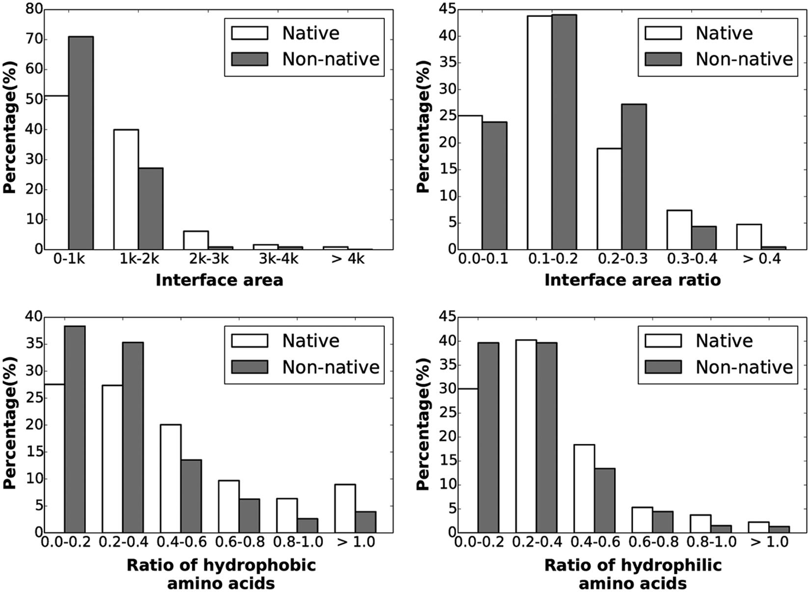
Distributions of the first 4/7 features/interaction properties over positive/native and negative/nonnative instances are shown here, in bar diagrams. The x axis represents the value range for the properties, and the y axis shows the percentage of instances that fall within a particular value range. Positive and negative instances are shown in white and diagonal lined bars, respectively.

FIG. 2.

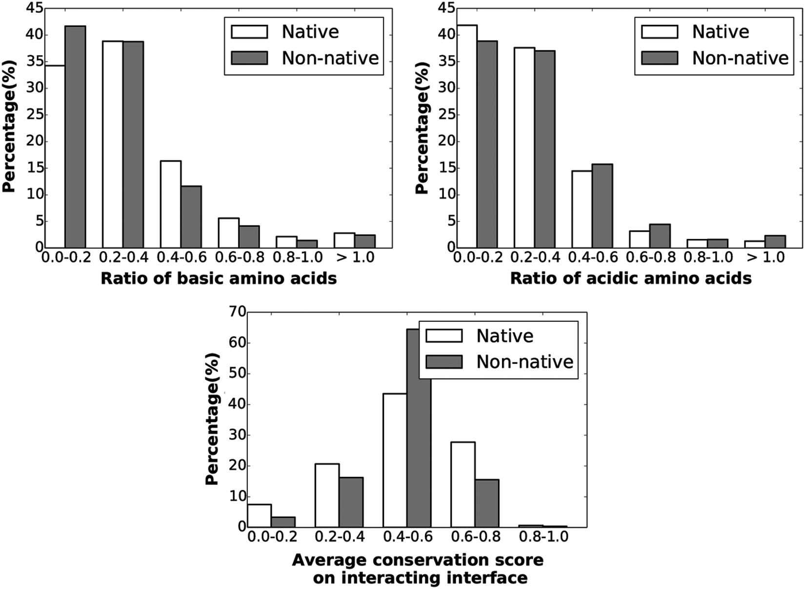
Distributions of the rest of the 3/7 features/interaction properties are shown here.

Figure 1 shows that the interface area of positive/native instances is overall higher than that of most negative instances, while no conclusive observations can be made regarding the interface area ratio. Native instances tend to have more hydrophobic atoms than nonnative ones, and a similar observation can be drawn regarding ratio of hydrophobic amino acids. On the other hand, acidic and basic compositions do not seem to discriminate between native and nonnative instances. One does observe more native than nonnative instances have average conservation scores >0.6.

2.4.4. Identification of optimal classification model

To summarize, the interaction interface in a training instance is first computed, and the interface is converted into a seven-entry vector as described above. Various classification models available in the weka software package (Hall et al., 2009) are then trained, and their performance is recorded in a 10-fold validation setting for the purpose of comparison.

The models trained and compared here are entropy-based decision tree (J48 implementation in weka), random forest, bagging, and support vector machines. The performance of each trained model is measured in terms of F-measure, precision, recall, and area under receiver operating characteristic (ROC) curves. We show here the ROC curves of each trained model in Figure 3. An ROC curve is generated by plotting the true positive rate against the false positive rate at different threshold settings. An area under the curve (AUC) of 1 represents a perfect prediction, while an AUC of 0.5 represents a random prediction.

FIG. 3.

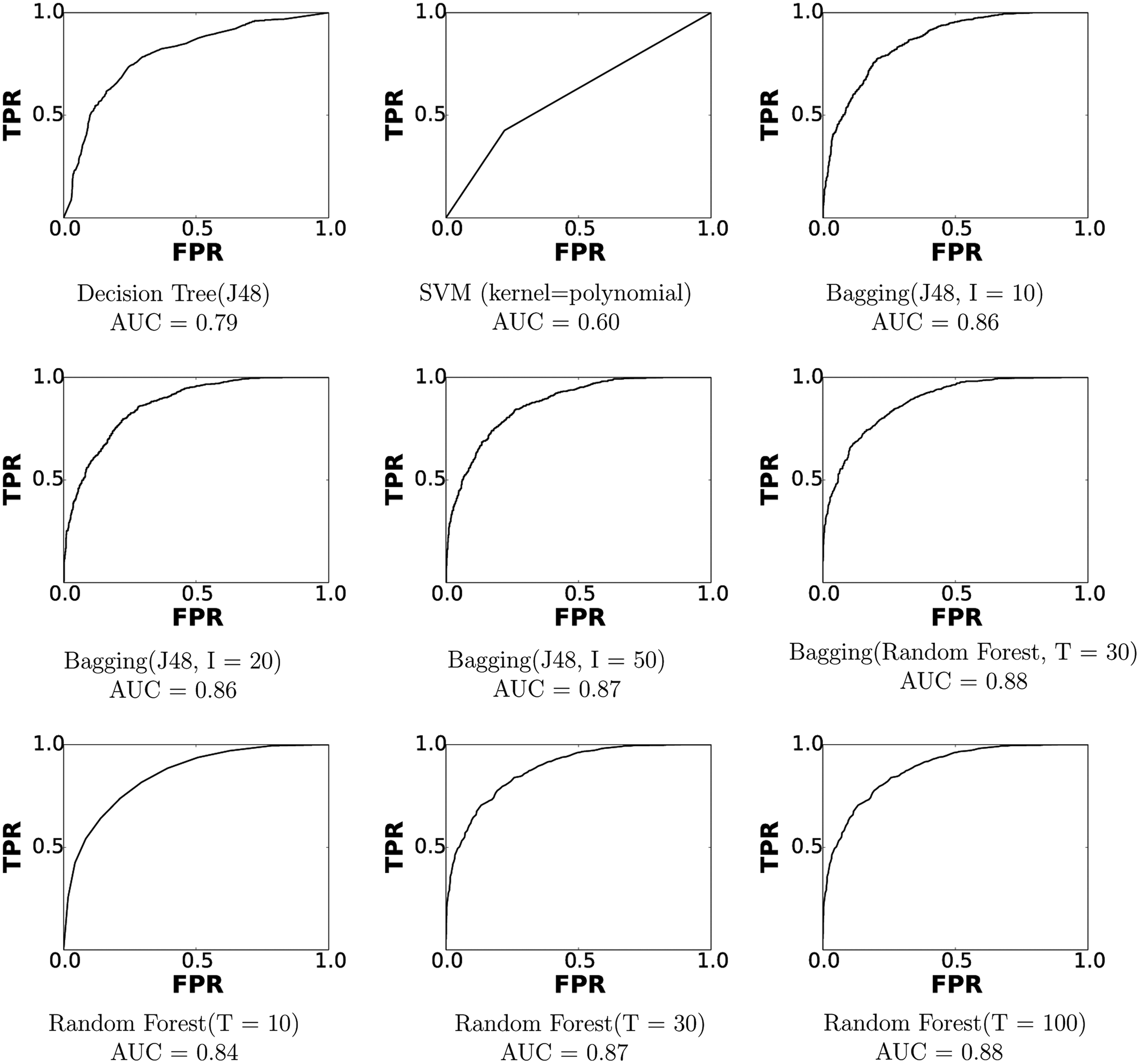
Receiver operating curves (ROCs) are shown for the different machine learning models. An area under the curve of 1.0 represents a perfect prediction while an area under the curve of 0.5 represents random guess. FPR, false positive rate; TRP, true positive rate; I, number of iterations; T, number of trees.

As shown in Figure 3, the J48 tree and SVM with polynomial kernel perform worse among all models. It is worth noting parameters of each model have been tuned in order to get the best performance from each. The performance of bagging and random forest tree models grow as the number of iterations I and number of trees T increase. However, model complexity for each grows, as well, and raises the possibility of model overfitting. Therefore, after the detailed comparison in terms of performance, timing, and model complexity, we have chosen bagging with I=10 and J48 as base classifiers for the learner integrated in idDock+. The AUC of this model is 0.86, which is very much comparable with the other more complex models shown in Figure 3.

3. Results

idDock+ is implemented in C/C++ and run on ARGO, a research computing cluster provided by the Office of Research Computing at George Mason University. Compute nodes used for testing are Intel Xeon E5-2670 CPU with 2.6GHz base processing speed and 3.5TB of RAM. Testing is conducted on 15 known protein dimers, detailed below. On each testing system, idDock+is run until either 10, 000 dimeric configurations are obtained or 7 days of CPU time have passed. This is repeated independently five times to account for probabilistic variance in the obtained results. Two different sets of analyses are conducted. First, the proximity of the configuration closest to the known native structure is reported for each system and compared to similar values reported by other state-of-the-art methods; other methods are also run five times in order to estimate variance of the results. Second, a more detailed analysis is conducted that looks at the relationship between energy and lRMSD to the known native structure to determine the likelihood of selecting a native-like configuration from energy-based selection mechanisms.

3.1. Performance measurements

One of the main measurements we employ here is root-mean-square-deviation (RMSD) to the known native dimeric structure to determine the quality of a generated configuration. RMSD is widely accepted now in docking methods and is reported in units of Å. RMSD measures the average atomic displacement between two configurations x and y under comparison: \documentclass{aastex}\usepackage{amsbsy}\usepackage{amsfonts}\usepackage{amssymb}\usepackage{bm}\usepackage{mathrsfs}\usepackage{pifont}\usepackage{stmaryrd}\usepackage{textcomp}\usepackage{portland, xspace}\usepackage{amsmath, amsxtra}\pagestyle{empty}\DeclareMathSizes{10}{9}{7}{6}\begin{document} \begin{align*}\sqrt { \frac { 1 } { N } \mathop \sum \limits_ { i = 1 } ^ { N } \parallel x_i - y_i \parallel^2 } \tag { 4 } \end{align*} \end{document}

least RMSD (lRMSD) refers to the minimum RMSD over all possible rigid-body motions of one configuration relative to the other. A value between 2 and 5Å typically indicates a configuration that is highly similar to the known native structure. We use lRMSD here not only to determine the proximity of dimeric configurations generated by idDock+ to the known native structure but also to analyze the rank at which the lowest lRMSD configuration is obtained over an energy-ascending sorted ordering of configurations.

3.2. Protein dimers selected for testing

Fifteen known dimers have been selected for testing. These dimers are chosen because they vary in size, functional classification, have been used by other docking methods to measure performance, and some have also been CAPRI targets. It is worth noting that the dimers are a testing dataset with no overlap with the training dataset used to train the ensemble learner incorporated in idDock+. The dimers are listed in Table 1, where column one shows the PDB identifier (ID) for each of the dimers followed by the chain identifiers in brackets. The next column shows the size of each of the chains in terms of total number of atoms. The last column shows the functional classification as obtained from the PDB (Berman et al., 2000).

Table 1.

Systems of Study

PDB ID (chains)	Size (no. of atoms)	Functional classification
1C1Y (A,B)	1376, 658	Signaling protein
1DS6 (A,B)	1413, 1426	Signaling protein
1TX4 (A,B)	1579, 1378	Complex (gtpase activation/proto oncogene)
1WWW (W,Y)	862, 782	Nerve growth factor/trka complex
1FLT (V,Y)	770, 758	Complex (growth factor/transferase)
1IKN (C,D)	916, 1589	Transcription factor
1VCB (A,B)	755, 692	Transcription
1VCB (B,C)	692, 1154	Transcription
1OHZ^* (A,B)	1027, 416	Cell adhesion
1ZHI^* (A,B)	1597, 1036	Transcription/replication
2HQS^* (A,C)	3127, 856	Transport protein/lipoprotein
1QAV (A,B)	663, 840	Membrane protein/oxidoreductase
1G4Y (B,R)	682, 1156	Signaling protein
1CSE (E,I)	1920, 522	Complex (serine proteinase inhibitor)
1G4U (R,S)	1398, 2790	Signaling protein

Details are listed here for each of the 15 dimers selected for testing. CAPRI targets are marked with an asterisk (✻). The size of each system is shown in terms of the total number of atoms. PDB, Protein Data Bank.

3.3. Comparative analysis

Here we summarize the performance of idDock+ on each testing dimer in terms of the lowest lRMSD over all configurations to the known native structure. The same value is obtained for other state-of-the-art methods from published data or from data we have obtained by running methods available in software or web server form. Methods from other labs to which we compare idDock+ are FTDock-pyDock (Jimenez-Garcia et al., 2013), ClusPro (Comeau et al., 2004), and ZDock (Pierce et al., 2014). ZDock, ClusPro, and pyDock are leading energy-driven methods. For completeness, we also compare idDock+ to one of our previous works, HopDock (Hashmi and Shehu, 2013a), for comparison. In HopDock, no machine learning model is integrated in the BH-based search, and a simple in-house energy function composed of van der Waals, electrostatic, and hydrogen bond terms is used. Each method is run five times on each protein system in order to estimate the variance between runs. It is worth noting that ZDock and ClusPro are deterministic methods.

Figure 4 summarizes the analysis comparing the lowest lRMSDs to the known native structure obtained from idDock+ and other state-of-the-art methods. Each method, idDock+ included, is run five times. The lowest lRMSD from each run of each method is recorded, and the range of lowest lRMSD values from all runs of all methods is plotted in gray Figure 4 for each of the test dimers. The range of lowest lRMSD values from the five runs of idDock+ is highlighted in black thicker line. Figure 4 clearly shows that even when considering variance between runs of all methods, idDock+ is one of the top performers in terms of the proximity to the known native structure for each of the test dimers. While idDock+ may not achieve the lowest lRMSD in each dimer (idDock+ achieves the lowest lRMSD on five dimers), the range of lowest lRMSDs obtained from different runs of it is in the bottom half of the range obtained from representative state-of-the-art methods.

FIG. 4.

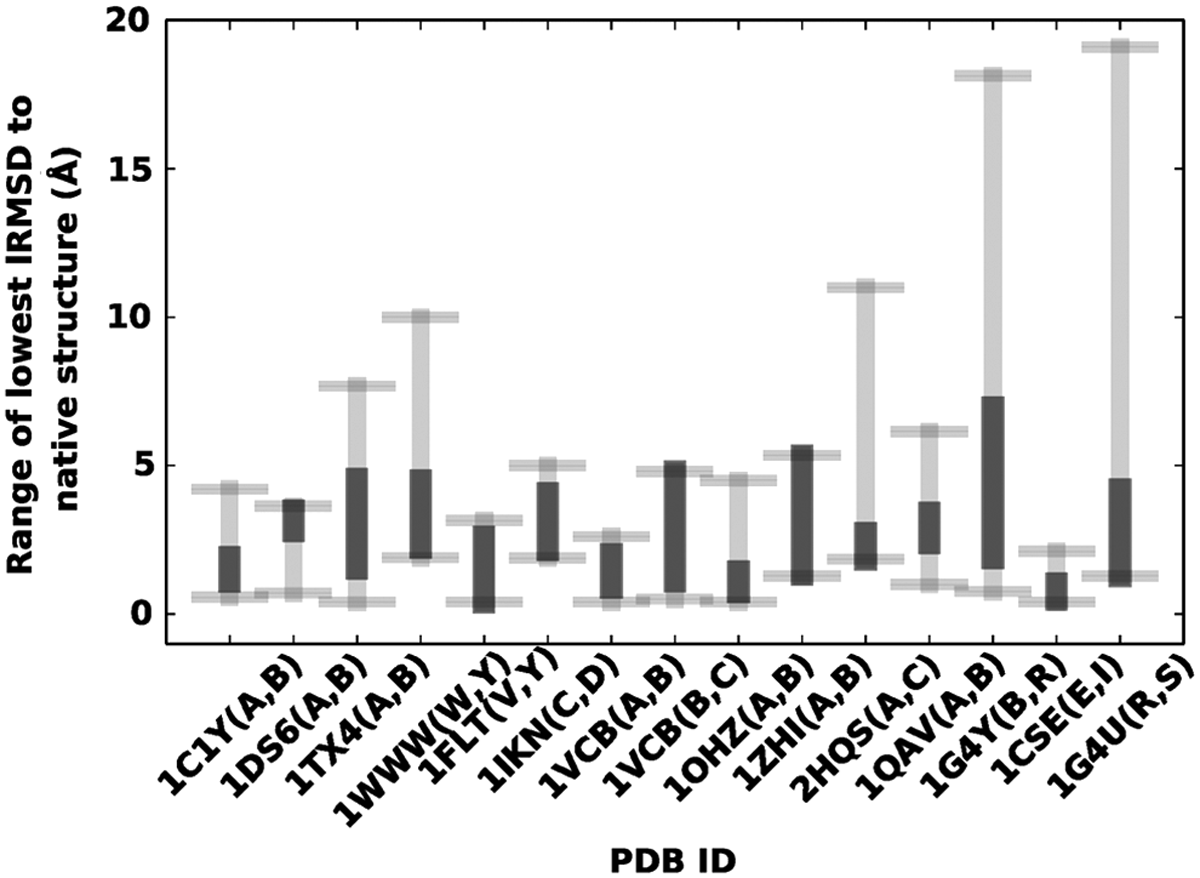
idDock+ is compared here to other state-of-the-art methods in terms of the lowest lRMSD (least root-mean-square-deviation) obtained to the native structure. Each method is run five times, and lowest lRMSDs obtained from all runs of all methods are combined to obtain a range, drawn in gray. The range of lowest lRMSDs obtained from all runs of idDock+ is highlighted in black.

The results summarized in Figure 4 effectively make the case for the contribution of the machine learning model in a probabilistic search algorithm such as idDock+. On some dimers, energy-driven methods are far off from the native structure (e.g., 1WWW, 2HQS, 1G4Y, and 1G4U), whereas idDock+ is able to report near-native structures on most systems (except 1ZHI and 1G4Y, where the lowest lRMSD obtained from idDock+ is slightly higher than 5Å). Taken together, this analysis supports the claim that energy alone is not sufficient to drive a probabilistic search to the native structure.

3.4. Selection-based analysis

In the following we take a closer look at the performance of idDock+ compared to other methods, particularly to understand what proximity to the native structure would be obtained by energy-based selection techniques. The baseline energy-based selection technique sorts configurations by energy, from lowest to largest, and then reports where in the sorted ordering the configuration with the lowest lRMSD to the native structure is found. This value is known as rank.

Figure 5 summarizes this comparative analysis in terms of rank. As before, each method, idDock+ included, is run five times, and the rank of the configuration with the lowest lRMSD to the native structure is recorded. For idDock+, this configuration is found by sorting sampled configurations by their FoldX energies. For other methods, we rely on reported ranks. Methods such as pyDock and ZDock report rank. Since ClusPro provides top clusters with a total of 100 top structures, the rank we report for ClusPro is that within the reported structures.

FIG. 5.

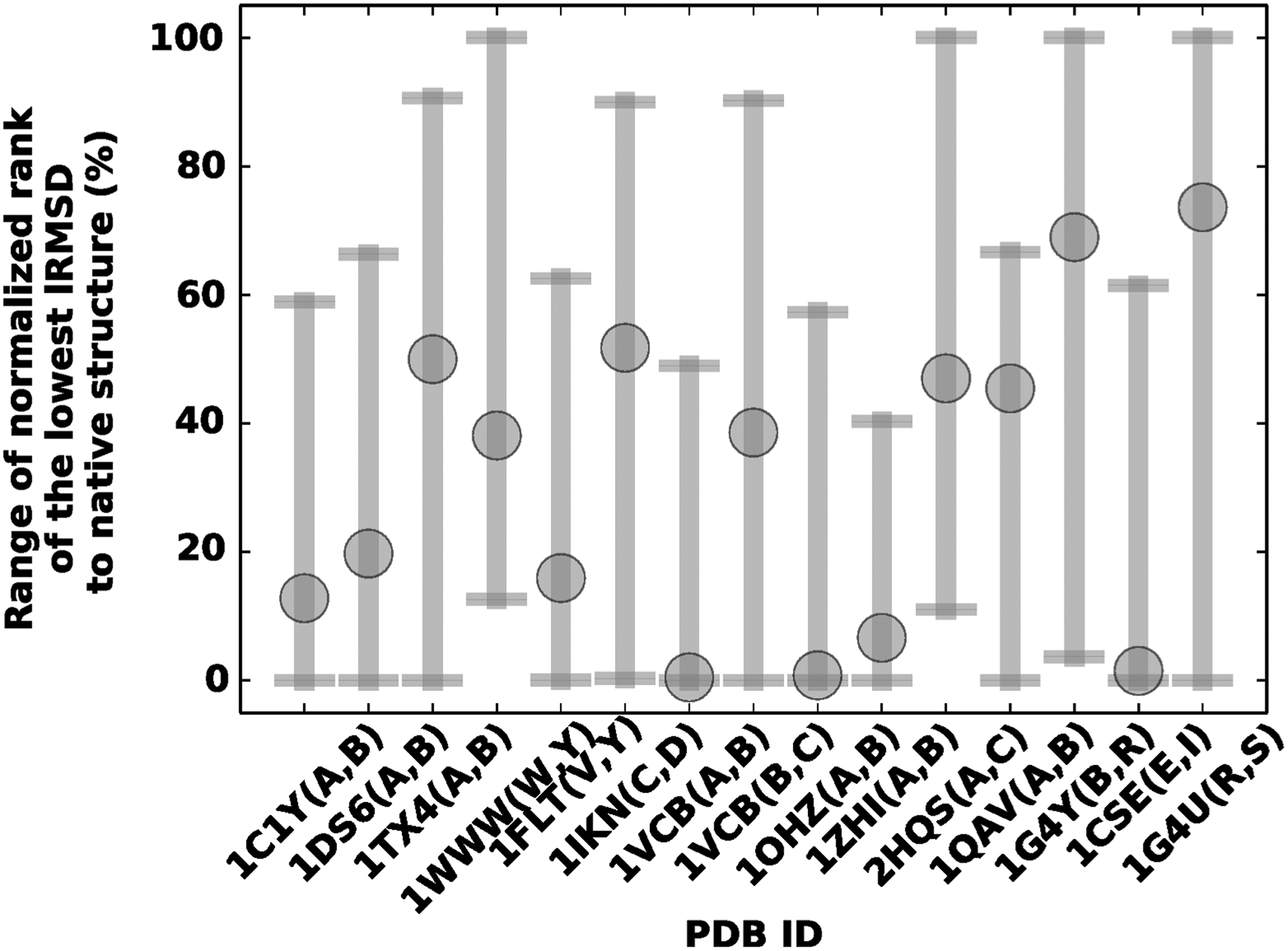
Normalized rank, measured as described above, is obtained from all runs of all methods. Its range is drawn in gray. The average normalized rank over five independent runs of idDock+ is highlighted, drawn as a gray circle.

Rather than reporting the absolute position in this ordering of the lowest-lRMSD-to-native configuration, we report a normalized location, dividing by the total number of configurations. This allows a fair comparison across the various dimers and various methods, which report a different number of their top solutions. In the case of idDock+, runs on some of the larger systems were terminated after 7 days. Cases where a rank of 100% is reported indicate those where the lowest lRMSD to the native structure is beyond a stringent threshold of 5Å. The normalized ranks of all five runs of all methods are combined for each system, and their range is drawn in gray in Figure 5. The average rank obtained over five independent runs of idDock+ is indicated through a gray circle.

Figure 5 shows that on 9/15 dimers, idDock+ shows comparable or better rank than other methods. These numbers include four dimers where three other methods are unable to find any solutions with lRMSDs less than 5Å. While not shown in detail, HopDock performs worst in terms of rank; this is due to a very simple energy function designed to guide the search in this method. For 7/15 of the dimers, the lowest-lRSMD idDock+-obtained configuration is among the top 20% of energy-sorted configurations. For some dimers, such as those with PDB ids 1OHZ, 1VCB(A, B), and 1CSE, a normalized rank of close to 0 is reported, which means that the lowest-energy configuration obtained by idDock+ is indeed the one with the lowest lRMSD to the native structure. Taken together, these results indicate that the machine learning model is effective at guiding the search in idDock+ toward the native structure, often working in concert with the energy function (a case-based analysis of this is provided below and in section 4).

We provide some more analysis as to why on some systems energy is a good selection criterion and on others it is not. Figure 6 plots FoldX energy versus lRMSD to the native structure for six selected dimers from a single run. Two dimers have been selected among those with very low rank; on these systems, energy is a good selection criterion. As Figure 6a and b shows, this is because there is some correlation between interaction energy and lRMSD at the lower values. Figure 6c and d shows the relationship between energy and lRMSD for two systems with higher ranks. Again, some correlation is observed. No correlation is found for the two systems shown in Figure 6e and f, which are selected among those with very high rank. On these systems, energy is not a discriminant.

FIG. 6.

Six systems have been selected on which to plot the FoldX interaction energy vs. lRMSD to the native structure of all idDock+-generated configurations. The two systems in (a)–(b) have very low rank, followed by low-rank systems in (c)–(d) and very high-rank ones in (e)–(f).

In Figure 7 we draw some of the lowest-lRMSD or lowest-energy configurations for selected systems from a randomly selected run of idDock+. Figure 7 superimposes these configurations over the corresponding native structure and draws them using visual molecular dynamics (VMD) (Humphrey et al., 1996). The chains are drawn in different black and gray, and the native structure is drawn in transparent. The top and middle panel in Figure 7 shows the lowest-lRSMD configurations for the six selected systems. The FoldX interaction energy and respective rank of the lowest-lRMSD configuration on each of these systems is also shown. The bottom panel in Figure 7 shows the lowest-energy configuration, instead, on three of the six selected systems. The lRMSD to the native structure of these configurations is also shown. On each of these three systems, the lowest-energy configuration is very far away from the native structure, including 1CSE (E, I), where a rank of 0.06 is found.

FIG. 7.

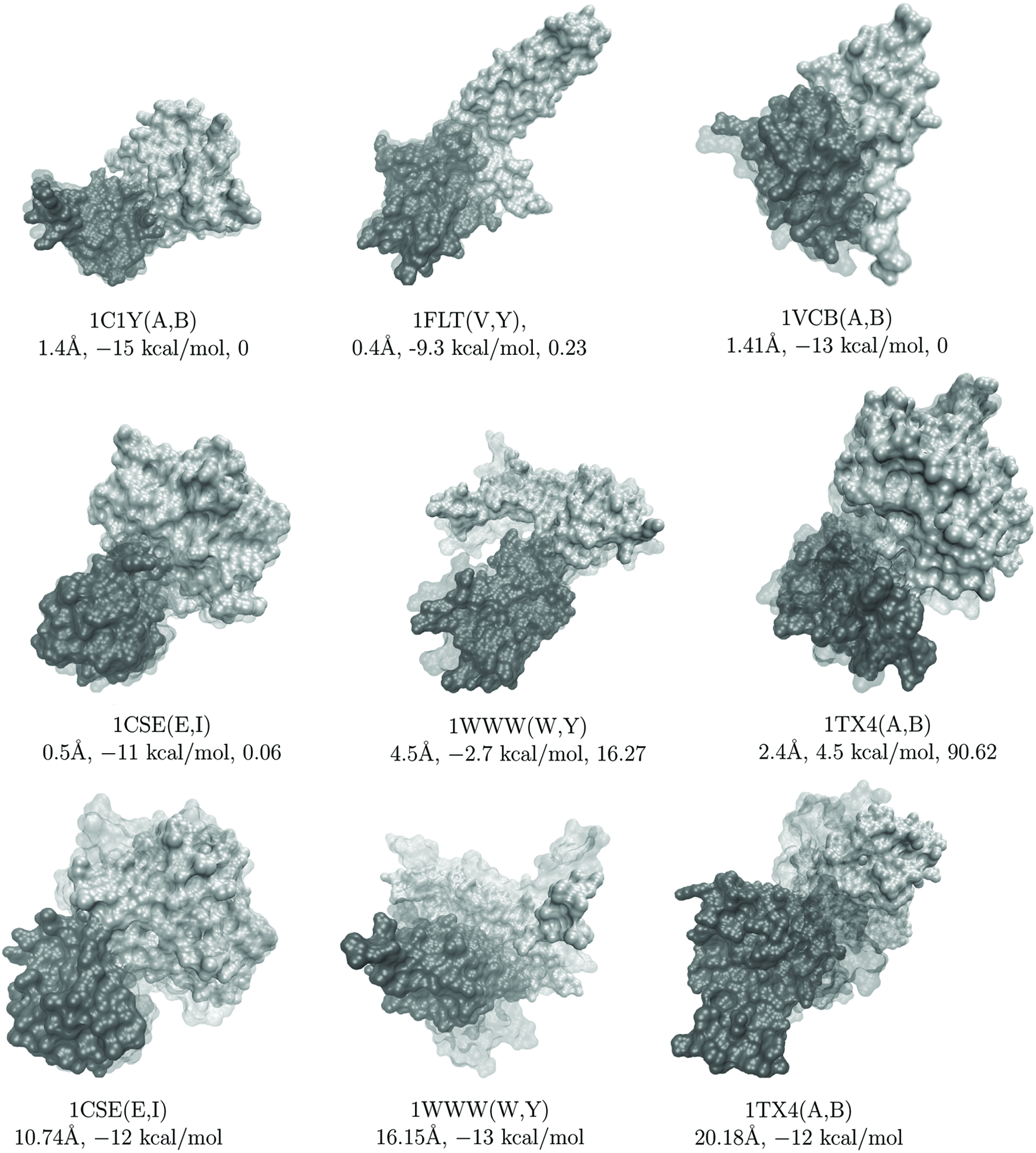
The bottom panel draws the lowest-energy configuration for three of the six selected systems (these configurations have rank 0). The lRMSD from the native structure is shown for each of these configurations. Chains are drawn in black and gray, and the native structure is drawn in transparent.

3.5. Timing profile

This section analyzes the timing profile of idDock+. We report the percentage of time each algorithmic component/operator in idDock+ needs using Gprof (Graham et al., 1982), a performance analysis tool for Unix-based applications. Reported values here are based on one single run and a randomly selected dimer (similar values are observed over different runs and different systems). Figure 8 shows that the local improvement operator, which makes use of the FoldX energy function, takes almost 80% of the running time. This time is spent on expensive energy evaluations. This is due to the fact that we employ a detailed and sophisticated energy function, FoldX, which on average takes about 0.39 seconds per configuration. Moreover, to generate one local minimum, idDock+ can iterate over k * m=1,000 energy evaluations. These evaluations are the main contributor to a running time of 7 CPU days on some of the largest dimers. On the other hand, only 8.0% of the running time is spent on the perturbation operator, which includes generating a random configuration and testing the relevancy of it through the predictive machine learning model. The rest of the time is spent on miscellaneous tasks like I/O operations, vector manipulations, and so on.

FIG. 8.

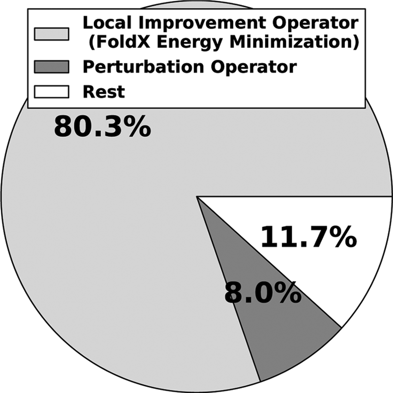
Timing profile of idDock+ is shown in a pie diagram. Different wedges show the percentage of time spent on different algorithmic components/operators in idDock+.

4. Discussion

We have presented here idDock+, a novel algorithm for sampling low-energy configurations in rigid-body protein–protein docking. The algorithm employs concepts from both geometry- and energy-driven methods. Its probabilistic search is a realization of the basin hopping framework that allows generating a metropolis Monte Carlo trajectory of consecutive local minima in the surface of a sophisticated energy function. However, one of the salient ingredients in idDock+ is its incorporation of a machine learning model to evaluate configurations prior to allocating to them a demanding budget for minimization. An ensemble learner is trained on a comprehensive training dataset and demonstrated effective in leading idDock+ toward near-native configurations.

In section 3 we focus on the overall performance of idDock+ and its comparison with other state-of-the-art methods that represent the various approaches to rigid protein–protein docking. Here we provide a few more details on why idDock+ succeeds or fails on certain systems. We focus on the relationship between the ensemble learner and the minimization with FoldX, as these two can work concertedly to lower the lRMSD to the native structure or against each other. We focus on four systems: one where the trained model performs well but nonetheless the energy function drives idDock+ away from the native structure; one where the trained model is inaccurate but the energy function nonetheless drives the search toward the native structure; one where both the trained model and the energy function work concertedly and lead idDock+ to the native structure; and one where both fail.

The first case is illustrated by the dimer with PDB id 1WWW, where the lowest lRMSD to the native structure is 4.5Å. On this system, the learned model performs well and evaluates as true configurations that have lRMSD to the native structure lower than 4.5Å. However, the energy function in the local improvement operator drives these configurations away from the native structure, resulting in an lRMSD higher than what the trained model would have reported in isolation. For instance, cases are found where the perturbed configuration that passes the stringent test of the learned model is less than 3.5Å in lRMSD to the native structure, but the minimization with FoldX modifies the configuration to one with higher lRMSD to the native structure.

The second case is illustrated by the dimer with PDB id 1VCB(A, B), where the lowest lRMSD to the native structure is 1.4Å. The particular configuration that achieves this lRMSD is obtained by minimizing a perturbed configuration that has passed the learned model but has lRMSD to the native structure of 6.40Å. This is an example where the energy function drives toward the native structure very effectively; the minimization lowers the interaction energy from 90.02 to −13kcal/mol. This represents an ideal case, where the best solution is obtained through energetic refinement.

The third case is illustrated by the dimer with PDB id 1FLT(V,Y), on which the learned model and the energy function perform in concert with each other. The configuration with the lowest lRMSD to the native structure is obtained from a perturbed configuration that has passed the learned model and has lRMSD of 3.61Å to the native structure. The minimization further lowers this lRMSD to 0.4Å, which is a significant improvement of 3Å.

The last case is illustrated by the system with PDB id 1G4Y(B,R), where neither the learned model nor the energy function are able to drive idDock+ toward low-lRMSD configurations. On this system, idDock+ obtains a lowest lRMSD to the native structure of 5.9Å.

To our knowledge, idDock+ represents one of the first algorithms that integrate learned models in probabilistic search or stochastic optimization for rigid protein–protein docking. Our results support the conclusion that this direction of research in protein–protein docking is worth investigating further, as the integration of an accurate learned model promises to address the issue with energy-driven optimization unable to solely drive the search toward near-native configurations. Consistently, studies show that energy-driven optimization is effective on configurations in the vicinity of the native structure. It is the premise of learned models to identify such configurations efficiently. The issue of efficiency is important, as our timing analysis shows that a significant percentage of computational time is spent on expensive energy evaluations, even when limiting the number of configurations sent for such evaluations through a machine learning model.

It is worth noting that the algorithm presented here offers a roadmap on how to integrate other machine learning models in stochastic optimization approaches to protein–protein docking. As our detailed investigation of four selected systems indicates, there is room for improvement both in machine learning models and energy functions. Growing work in machine learning is expected to lead to more accurate models possibly able to discriminate against more false positives. These, coupled with increasingly accurate energy functions and enhanced sampling strategies, are expected to lead to further improvements in protein–protein docking.

Footnotes

Acknowledgments

Computations were run on ARGO, a research computing cluster provided by the Office of Research Computing at George Mason University, Virginia. Funding for this work is provided in part by the National Science Foundation (CAREER Award No. 1144106). The authors are also grateful to members of the Shehu lab for useful feedback during this work.

Authors' Contributions

I.H. and A.S. conceived the algorithm proposed here, as well as the experimental design and the analysis strategy. I.H. implemented the algorithm, performed production runs, and carried out data analysis. I.H. and A.S. wrote the article.

Author Disclosure Statement

The authors declare that no competing financial interests exist.

References

Bajaj

C.L.

, Chowdhury

, and Siddahanavalli

2011. F2dock: fast fourier protein-protein docking. IEEE/ACM Trans. Comp. Biol. Bioinf., 8, 45–58.

Berman

H.M.

, Westbrook

, Feng

, et al. 2000. The Protein Data Bank. Nucleic Acids Res. 28, 235–242.

Bordner

A.J.

, and Gorin

A.A.

2007. Protein docking using surface matching and supervised machine learning. Proteins Struct. Funct. Bioinf., 68, 488–502.

Chen

, Li

, and Weng

2003. ZDock: an initial-stage protein-docking algorithm. Proteins Struct. Funct. Genet., 52, 80–87.

Cheng

T.M.

, Blundell

T.L.

, and Fernandez-Recio

2007. pyDock: electrostatics and desolvation for effective scoring of rigid-body protein–protein docking. Proteins Struct. Funct. Bioinf., 68, 503–515.

Comeau

S.R.

, Gatchell

D.W.

, Vajda

, and Camacho

C.J.

2004. ClusPro: a fully automated algorithm for protein-protein docking. Nucleic Acids Res., 32, W96–W99.

Connolly

M.L.

1983. Analytical molecular surface calculation. J. Appl. Cryst., 16, 548–558.

Dominguez

, Boelens

, and Bonvin

A.M.

2003. Haddock: a protein-protein docking approach based on biochemical orbiophysical information. J. Am. Chem. Soc., 125, 1731–1737.

Duhovny-Schneidman

, Inbar

, Nussinov

, and Wolfson

H.J.

2005. PatchDock and SymmDock: servers for rigid and symmetric docking. Nucleic Acids Res. 33, W363–W367.

10.

Engelen

, Ladislas

A.T.

, Sacquin-More

, et al. 2009. A largescale method to predict protein interfaces based on sequence sampling. PLoS Comput. Biol., 5, e1000267.

11.

Fischer

, Lin

S.L.

, Wolfson

H.L.

, and Nussinov

2005. A geometry-based suite of molecular docking processes. J. Mol. Biol. 248, 459–477.

12.

Graham

S.L.

, Kessler

P.B.

, and Mckusick

M.K.

1982. Gprof: a call graph execution profiler. ACM Sigplan Notices. 17, 120–126.

13.

Hall

, Frank

, Holmes

, et al. 2009. The weka data mining software: an update, 10–18. ACM SIGKDD, volume 11. ACM, New York, NY.

14.

Halperin

, Ma

, Wolfson

, and Nussinov

2002. Principles of docking: an overview of search algorithms and a guide to scoring functions. Proteins Struct. Funct. Genet. 47, 409–443.

15.

Hashmi

, and Shehu

2012. A basin hopping algorithm for protein-protein docking, 466–469. IEEE International Conference on Bioinformatics and Biomedicine (BIBM). IEEE, Philadelphia, PA.

16.

Hashmi

, and Shehu

2013a. Hopdock: a probabilistic search algorithm for decoy sampling in protein-protein docking. Proteome Sci., 11, S6.

17.

Hashmi

, and Shehu

2013b. Informatics-driven protein-protein docking, 772–779. ACM Conference on Bioinformatics and Computational Biology Workshops (BCBW). ACM, Washington, DC.

18.

Hashmi

, Akbal-Delibas

, Haspel

, and Shehu

2011. Protein docking with information on evolutionary conserved interfaces, 358–365. IEEE International Conference on Bioinformatics and Biomedicine Workshops (BIBMW). IEEE, Atlanta, GA.

19.

Hashmi

, Akbal-Delibas

, Haspel

, and Shehu

2012. Guiding protein docking with geometric and evolutionary information. J. Bioinf. Comp. Biol., 10, 1242002.

20.

Huang

2014. Search strategies and evaluation in protein–protein docking: principles, advances and challenges. Drug Discov. Today, 19, 1081–1096.

21.

Humphrey

, Dalke

, and Schulten

1996. VMD— visual molecular dynamics. J. Mol. Graph., 14, 33–38.

22.

Inbar

, Benyamini

, Nussinov

, and Wolfson

H.J.

2005. Combinatorial docking approach for structure prediction of large proteins and multi-molecular assemblies. J. Phys. Biol., 2, S156–S165.

23.

Jimenez-Garcia

, Pons

, and Fernandez-Recio

2013. pyDockWEB: a web server for rigid-body protein-protein docking using electrostatics and desolvation scoring. Bioinformatics, 29, 1698–1699.

24.

Kanamori

, Murakami

, Tsuchiya

, et al. 2007. Docking of protein molecular surfaces with evolutionary trace analysis. Proteins Struct. Funct. Bioinf., 69, 832–838.

25.

Kilambi

K.P.

, Reddy

, and Gray

J.J.

2014. Protein-protein docking with dynamic residue protonation states. PLoS Comput. Biol., 10, e1004018.

26.

Kozakov

, Brenke

, Comeau

, and Vajda

2006. PIPER: an FFT-based protein docking program with pairwise potentials. Proteins Struct. Funct. Bioinf., 65, 392–406.

27.

Lensink

M.F.

, and Wodak

S.J.

2009. Docking and scoring protein interactions: CAPRI 2009. Proteins Struct. Funct. Bioinf., 78, 3073–3084.

28.

, and Kihara

2012. Protein docking prediction using predicted protein-protein interface. BMC Bioinf., 13, 7.

29.

, Sun

, and Jiang

2008. Prediction of protein-protein binding site by using core interface residue and support vector machine. BMC Bioinf., 9, 553.

30.

Lin

S.L.

, Nussinov

, Fischer

, and Wolfson

H.J.

1994. Molecular surface representations by sparse critical points. Proteins Struct. Funct. Genet., 18, 94–101.

31.

Lyskov

, and Gray

J.J.

2008. The RosettaDock server for local protein-protein docking. Nucleic Acids Res. 36, W233–W238.

32.

Macindoe

, Mavridis

, Venkatraman

, et al. 2010. Hexserver: an FFT-based protein docking server powered by graphics processors. Nucleic Acids Res., 38, W445–W449.

33.

Moitessier

, Englebienne

, Lee

, et al. 2009. Towards the development of universal, fast and highly accurate docking/scoring methods: a long way to go. Br. J. Pharmacol., 153, S7–S27.

34.

Olson

, Hashmi

, Molloy

, and Shehu

2012. Basin hopping as a general and versatile optimization framework for the characterization of biological macromolecules. Adv. AI J., 2012, 674832.

35.

Pierce

B.G.

, Wiehe

, Hwang

, et al. 2014. ZDOCK server: interactive docking prediction of protein–protein complexes and symmetric multimers. Bioinformatics, 30, 1771–1773.

36.

Ritchie

D.W.

2008. Recent progress and future directions in protein-protein docking. Curr. Protein Pept. Sci., 9, 1.

37.

Schymkowitz

, Borg

, Stricher

, et al. 2005. The foldx web server: an online force field. Nucleic Acids Res., 33, W382–W388.

38.

Shoemaker

B.A.

, and Panchenko

A.R.

2007. Deciphering protein–protein interactions. Part II. Computational methods to predict protein and domain interaction partners. PLoS Comput. Biol., 3, e43.

39.

Terashi

, Takeda-Shitaka

, Kanou

, et al. 2007. The SKE-DOCK server and human teams based on a combined method of shape complementarity and free energy estimation. Proteins Struct. Funct. Bioinf., 69, 866–887.

40.

Tovchigrechko

, and Vakser

I.A.

2006. GRAMM-X public web server for protein-protein docking. Nucleic Acids Res., 34, W310–W314.

41.

Wales

D.J.

, and Doye

J.P.K.

1997. Global optimization by basin-hopping and the lowest energy structures of lennard-jones clusters containing up to 110 atoms. J. Phys. Chem. A, 101, 5111–5116.

42.

Wang

, Fang

, Lu

, et al. 2005. The pdbbind database: methodologies and updates. J. Med. Chem., 48, 411–419.

43.

Yan

, Dobbs

, and Honavar

2004. A two-stage classifier for identification of protein–protein interface residues. Bioinformatics, 20, i371–i378.

44.

Zhu

, Domingues

F.S.

, Sommer

, and Lengauer

2006. NOXclass: prediction of proteinprotein interaction types. BMC Bioinf., 7, 27.

idDock+: Integrating Machine Learning in Probabilistic Search for Protein–Protein Docking

Abstract

Abstract

1. Introduction

2. Methods

2.1. Rigid-body transformations to obtain docked configurations in idDock+

2.2. Perturbation operator in idDock+

2.3. Local improvement operator in idDock+

2.4. Machine learning model to evaluate perturbed configurations in idDock+

2.4.1. Training dataset

2.4.2. Feature vector

2.4.3. Analysis of interaction properties

2.4.4. Identification of optimal classification model

3. Results

3.1. Performance measurements

3.2. Protein dimers selected for testing

3.3. Comparative analysis

3.4. Selection-based analysis

3.5. Timing profile

4. Discussion

Footnotes

Acknowledgments

Authors' Contributions

Author Disclosure Statement

References