Conformational Sampling Reveals Amino Acids with a Steric Influence on Specificity

Abstract

Flexible representations of protein structures can enable structure comparison algorithms to find remotely homologous proteins, even when they have been crystallized in different conformations. By compensating for large spatial variations, these representations can enable these algorithms to better detect remote similarities in the space of protein structures. Subtle variations in protein structures can also have a substantial impact structure comparison. For example, the motion of a single side chain into a binding cavity can make the cavity appear totally dissimilar to identical binding sites, even though, in reality, the presence of the side chain does not affect binding. To address the impact of subtle conformational variations, this article describes FAVA (Flexible Aggregate Volumetric Analysis), an algorithm that enables comparisons of ligand binding sites while compensating for subtle, localized flexibility.

FAVA integrates hundreds of conformational samples, sourced from any molecular simulation software that provides all-atom detail, to characterize the geometry of ligand binding sites as they frequently appear. This representation enables rare conformations, as defined by the user, to be excluded from the structural comparison. In our results, on three families of serine proteases and three families of enolases, we show that despite substantial binding site variations, FAVA is able to correctly classify families with different binding preferences. We also demonstrate that FAVA can examine the motion of individual amino acids to identify those that influence ligand binding specificity. Together, these capabilities demonstrate that comparison errors associated with small conformational variations, which can substantially alter the geometry of ligand binding sites and other local features, can be mitigated by an analysis of many conformational samples.

1. Introduction

Algorithms that compare protein structures have generally focused on the identification of proteins with similar functions at great evolutionary distances. Aiming to reveal the topology of the space of protein structures (Murzin et al., 1995; Orengo et al., 1997; Holm and Sander, 1994; Yang and Honig, 2000), many algorithms specialize in identifying proteins with backbone similarities that can point to shared evolutionary origins, even when similarity is not apparent from amino acid sequences alone (Nussinov and Wolfson, 1991; Orengo and Taylor, 1996; Holm and Sander, 1996; Russell, 1998; Shindyalov and Bourne, 1998; Zhang and Skolnick, 2005). In such cases, proteins that have been crystalized in different conformations can be overlooked, because the spatial relationships between their constituent parts can appear quite different. To compensate for conformational variations, some methods employ flexible representations of proteins as collections of rigid components with flexible linkers. These representations employ hinges (Shatsky et al., 2004; Gunasekaran and Nussinov, 2007), graph structures (Ye and Godzik, 2005; Konc and Janežič, 2010), fragments (Mosca and Schneider, 2008), and dynamic programming (Vesterstrøm and Taylor, 2006; Birzele et al., 2007; Menke et al., 2008) to avoid discarding similar proteins in alternate conformations.

Comparisons of smaller elements of protein structure, such as ligand binding cavities (Russell, 1998; Binkowski et al., 2004; Chen et al., 2007; Bryant et al., 2013), are also affected by small conformational variations. While large changes, such as backbone motions, still disrupt the comparison of ligand binding cavities (Godshall and Chen, 2012; Godshall et al., 2013), smaller variations, such as the motion of individual side chains, also cause similar binding cavities to appear very different. This second source of error disrupts the search for proteins with similar binding sites at great evolutionary distances (Chen et al., 2005; Stark et al., 2003; Dundas et al., 2011; Bryant et al., 2013), and also the identification of binding site variations that cause differences in ligand binding specificity (Chen and Honig, 2010; Guo et al., 2014; Guo and Chen, 2014). While flexible representations can compensate for large variations in backbone geometry, existing methods do not compensate for the large space of smaller motions that disrupt local comparisons.

To address this problem, we describe a method for reducing comparison errors due to small variations in protein structure called FAVA (Flexible Aggregate Volumetric Analysis). FAVA integrates structural data from many conformational samples to create a volumetric representation of binding cavity regions (frequent regions) that are frequently accessible to solvent. In our results we will show that comparisons of frequent regions can reveal differences between binding cavities that explain different binding preferences, even though many conformational variations can obscure this trend. We will also demonstrate that comparisons of many conformations of individual amino acids with the binding cavities of other proteins can precisely reveal amino acids that have a steric influence on ligand binding specificity, even though many amino acids occasionally interfere with binding cavity shape. FAVA demonstrates that an aggregate analysis of many conformational samples can yield insights into conformational trends for localized comparison.

Sampled conformations exhibit a novel advantage. All-atom samples provide a more detailed representation of molecular motion than that provided by existing methods. In each sample, the position of every atom is affected by energy functions that enforce biophysical constraints. Each relevant atom can thus be used for constructing a semirealistic representation of binding site geometry. In constrast, existing methods approximate rigidity in some places and flexibility in others. While the same biophysical constraints are not in effect, the computational expense of molecular simulation is also not necessary in existing methods. Detailed biophysical semirealism is thus achieved in exchange for the substantial computational cost of conformational sampling. While more sophisticated methods could be applied (e.g., Olson and Shehu, 2012) our tradeoff specializes FAVA for the detailed comparison of ligand binding cavities, where the motion of every atom is critical, whereas the detection of similar proteins with large conformational variations, which would be expensive to simulate anyway, is best suited for the rigid components and flexible linkers used in existing work.

Frequent regions are generated using Boolean operations from constructive solid geometry (CSG) (Chen and Honig, 2010), such as union, intersection, and difference (Fig. 1a). CSG operations are also used to compare binding cavities and identify potentially influential amino acids. CSG intersections between frequent regions identify conserved frequent regions, which describe regions in the binding cavities of two structurally aligned proteins that are frequently solvent accessible in both proteins. These regions might accommodate molecular fragments common to substrates that bind both proteins. CSG differences between frequent regions identify unconserved frequent regions, which represent regions in aligned binding cavities that are frequently solvent accessible in one protein but not the other. Unconserved frequent regions might therefore accommodate ligands in one protein that cannot bind in another and thereby have a steric influence on specificity. Finally, CSG operations permit the identification of amino acids that frequently alter cavity shape, and thus have a steric influence on specificity. Together, these techniques create a conformationally general approach for examining closely related proteins in search of influences on binding specificity.

FIG. 1.

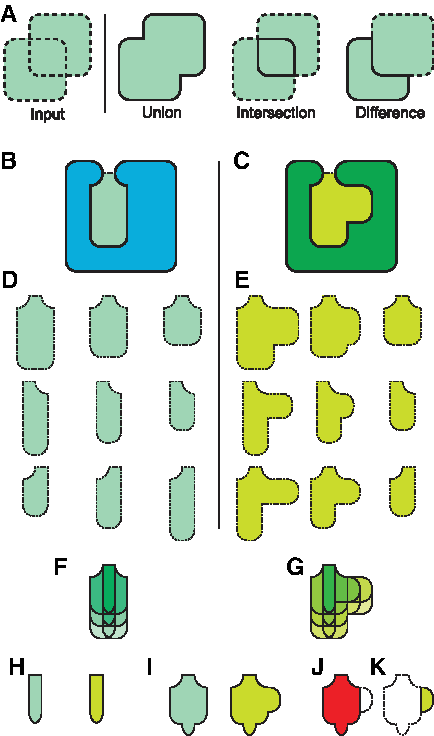
An overview of the FAVA method. (A) CSG operations used by FAVA, with input regions (green, dotted outline) and output regions (solid outline). (B,C) Input proteins X (blue) and Y (green) with ligand binding sites x (light green) and y (yellow). (D,E) x and y in different conformational samples. (F,G) All conformational samples of x (transparent green) and y (transparent yellow), superposed, with black outlines. Considerable variations in cavity shape are apparent. (H) Using CSG, the intersection of all cavity regions in both proteins is too small to accommodate ligands. They are also identical, revealing little about different binding preferences. (I) Using CSG, FAVA approximates frequent regions, where every point is inside at least two thirds of all samples of x (green) and y (yellow). (J) The intersection of frequent regions indicates regions that might accommodate similar molecular fragments (red). (K) The difference between frequent regions (yellow) indicates a region where Y might often accommodate a ligand that X cannot, causing a difference in specificity.

In earlier work (Guo et al., 2014), we demonstrated that comparisons of frequent regions generated with FAVA could reveal patterns of subtle differences in binding cavities that relate to ligand binding preferences. We also showed examples demonstrating that amino acids that frequently alter cavity shape have a steric influence on specificity. This article summarizes the methods employed by FAVA and extends our earlier examples, providing a comprehensive study of the conformational variation of all amino acids within a sequentially nonredundant set of serine proteases.

2. Methods

Below, we paraphase methods associated with FAVA that we described earlier (Guo et al., 2014). FAVA defines frequent regions as regions in space that are solvent accessible in more than k/N samples, where k, the overlap threshold, is provided as input, and N is the number of samples. By setting k, the user defines how frequently a region in space must be solvent accessible in order to be part of the frequent region. Unusual gaps and clefts that occur less frequently than k/N will thus not be reflected in the shape of the frequent region. We first describe how frequent regions are computed using CSG operations, employing the symbols ∪, ∩, and – to represent CSG unions, intersections, and differences, respectively. Implementation of individual CSG operations has been described earlier (Chen and Honig, 2010). Next, we describe how frequent regions from multiple proteins are compared using CSG operations. Finally, we explain how we use sampled conformations of individual amino acids to assess their steric impingement on nearby binding cavities.

2.1. Computing frequent regions

To generate a frequent region, we begin with the overlap threshold k, N conformational samples of a protein structure A, and a ligand l bound to the structure of A (Fig. 2b). We use A₀, A₁, … A_N to refer to conformational samples of A, which could be provided from any source that specifies all atom positions. It is asssumed that enough samples have been gathered so that the range of short timescale motions, such as sidechain movements, are represented in the samples. Beginning with this data, we follow two steps to generate frequent regions: First, we define the ligand binding cavity in every sample, and second, we analyze these cavities to determine the shape of the frequent region.

FIG. 2.

Generating frequent regions. (A) Conformational samples A₀, A₁,…A_N of protein A, shown as molecular surfaces (teal, black outlines). (B) Ligand l (red dots) bound to protein A (green). (C) Aligning each A_i to A permits l to mark the ligand binding site in A_i. (D) Spheres that define the neighborhood around the atoms of l (transparent blue, black outlines). (E) CSG union of the spheres, S_l (blue). (F) CSG difference \documentclass{aastex}\usepackage{amsbsy}\usepackage{amsfonts}\usepackage{amssymb}\usepackage{bm}\usepackage{mathrsfs}\usepackage{pifont}\usepackage{stmaryrd}\usepackage{textcomp}\usepackage{portland, xspace}\usepackage{amsmath, amsxtra}\pagestyle{empty}\DeclareMathSizes{10}{9}{7}{6}\begin{document} $$A_i^{ \prime}$$ \end{document} that removes the region within the molecular surface of each A_i (dotted outline) from copies of S_l. (G) Envelope surfaces (yellow, black lines) and molecular surfaces (dotted lines) of all A_i. (H) Envelope surfaces aligned. Outlines of all envelopes are shown in black. (I) The global envelope region, E(A), generated with CSG intersections (yellow, heavy black outline). (J) CSG intersection between each \documentclass{aastex}\usepackage{amsbsy}\usepackage{amsfonts}\usepackage{amssymb}\usepackage{bm}\usepackage{mathrsfs}\usepackage{pifont}\usepackage{stmaryrd}\usepackage{textcomp}\usepackage{portland, xspace}\usepackage{amsmath, amsxtra}\pagestyle{empty}\DeclareMathSizes{10}{9}{7}{6}\begin{document} $$A_i^{ \prime}$$ \end{document} , shown in blue, and E(A) (transparent yellow, black outline). (K) Cavities a_i defined on each conformational sample. (L) Cavity borders superposed (black outlines). (M) Frequent region that overlaps at least three cavities (red). (N) CSG intersections^* between several pairs of a_i. (O) The CSG union of intersections in N: \documentclass{aastex}\usepackage{amsbsy}\usepackage{amsfonts}\usepackage{amssymb}\usepackage{bm}\usepackage{mathrsfs}\usepackage{pifont}\usepackage{stmaryrd}\usepackage{textcomp}\usepackage{portland, xspace}\usepackage{amsmath, amsxtra}\pagestyle{empty}\DeclareMathSizes{10}{9}{7}{6}\begin{document} $$\alpha_{k}^{ \star}$$ \end{document} , the approximated frequent region (teal) overlapping at least two cavities.

We begin by superimposing every sample A_i onto A by computing a backbone superposition. Sophisticated algorithms designed to detect remote homologs (e.g., Nussinov and Wolfson, 1991; Orengo and Taylor, 1996; Holm and Sander, 1996; Shindyalov and Bourne, 1998; Zhang and Skolnick, 2005) are not necessary, because the proteins in A_i are identical to A, except in their conformation. For this reason, we compute a superposition that minimizes the root mean squared distance between identical atoms (Umeyama, 1991). Next, we generate the molecular surface m(A_i) of every conformational sample A_i, using GRASP2 (Petrey and Honig, 2003) (Fig. 2a). GRASP2 uses the classical rolling probe algorithm (Connolly, 1983) and the standard probe size of 1.4Å.

Now, since every A_i has been superposed onto A, the binding cavity of A is now approximately superposed with itself in every sample, so we use the ligand l, as bound in A, to represent the neighborhood of the binding site in every surface m(A_i) (Fig. 2c). Specifically, we define a sphere of radius 5Å, centered at every atom in l (Fig. 2d), and compute the CSG union of all these spheres. This neighborhood, S_l (Fig. 2e), defines the vicinity of the ligand binding cavity in every sample.

Next, we use S_l to define the binding cavity in every sample. First, we make a copy of S_l for every A_i and compute the CSG difference, A′_i=S_l−m(A_i), revealing part of the cavity (Fig. 2f). We also make an envelope surface, e(A_i), for every sample. Here, we again use GRASP2, which uses the same rolling probe method except that the probe radius is changed to 5.0 Å (Fig. 2g). This larger probe is 10 Å in diameter, so it does not roll into small clefts and cavities. For this reason, we use the resulting surface e(A_i) to define a logical exterior boundary between the cavity and the solvent. Since e(A_i) can vary significantly between different conformational samples, especially because of solvent-facing side chains (Fig. 2g) unrelated to cavity shape, we mitigate these differences by computing their intersection (Fig. 2h and i), \documentclass{aastex}\usepackage{amsbsy}\usepackage{amsfonts}\usepackage{amssymb}\usepackage{bm}\usepackage{mathrsfs}\usepackage{pifont}\usepackage{stmaryrd}\usepackage{textcomp}\usepackage{portland, xspace}\usepackage{amsmath, amsxtra}\pagestyle{empty}\DeclareMathSizes{10}{9}{7}{6}\begin{document} \begin{align*}E ( A ) = \bigcap_{ \forall i} e ( A_i ). \tag{1}\end{align*} \end{document}

As the intersection of the envelopes from all conformational samples, we refer to E(A) as the global envelope region. Note here that because our samples are generated at a medium timescale, and thus exclude large backbone motions, the shape of E(A) is not strongly influenced by backbone motion. Next, for every i, we compute the CSG intersection of \documentclass{aastex}\usepackage{amsbsy}\usepackage{amsfonts}\usepackage{amssymb}\usepackage{bm}\usepackage{mathrsfs}\usepackage{pifont}\usepackage{stmaryrd}\usepackage{textcomp}\usepackage{portland, xspace}\usepackage{amsmath, amsxtra}\pagestyle{empty}\DeclareMathSizes{10}{9}{7}{6}\begin{document} $$A_i^{ \prime}$$ \end{document} and E(A) (Fig. 2j). The result is the binding cavity in every conformational sample, which we call a_i (Fig. 2k).

Once we have determined the shape of the binding cavity in each conformational sample, we then use all a_i to approximate the frequent region α_k. Here, it is crucial to note that α_k is not practical to compute explicitly on a protein with many sampled conformations. Consider, for example, the simple case of k=30. The region α₃₀ includes the CSG intersection of a₀, a₁, a₂,… , a₃₀, because any point inside all of these regions is inside at least 30 a_i, and thus inside α₃₀. The same is true for any thirty member subset of {a₀, a₁, … , a_N}, so α₃₀ is the union of all intersections of thirty distinct sample cavities: \documentclass{aastex}\usepackage{amsbsy}\usepackage{amsfonts}\usepackage{amssymb}\usepackage{bm}\usepackage{mathrsfs}\usepackage{pifont}\usepackage{stmaryrd}\usepackage{textcomp}\usepackage{portland, xspace}\usepackage{amsmath, amsxtra}\pagestyle{empty}\DeclareMathSizes{10}{9}{7}{6}\begin{document} $$\left(N \atop 30 \right)$$ \end{document} intersections. Where N is several hundred samples and k is nontrivial, the exponential size of the calculation is clearly impractical, given the number of combinations.

Even though an explicit computation of α_k would be impractical, it can still be rapidly approximated. For any k, we select 500 random and distinct subsets of {a₀, a₁, … , a_N} of size k. Next, we compute the intersection of the binding cavities in each subset, and then the union of all such intersections. We call this region \documentclass{aastex}\usepackage{amsbsy}\usepackage{amsfonts}\usepackage{amssymb}\usepackage{bm}\usepackage{mathrsfs}\usepackage{pifont}\usepackage{stmaryrd}\usepackage{textcomp}\usepackage{portland, xspace}\usepackage{amsmath, amsxtra}\pagestyle{empty}\DeclareMathSizes{10}{9}{7}{6}\begin{document} $$\alpha_k^{ \star}$$ \end{document} . Figure 2n illustrates a small example of this process on a random selection). We tried random selections of different sizes (Guo et al., 2014) and found that frequent regions approximated from random subsets of 500 had consistent volumes, and therefore deemed 500 sampled subsets to be sufficient for accurate representations.

2.2. Comparing frequent regions

To compare frequent regions representing the binding cavities of two proteins, A and B, we begin by aligning B onto A using ska (Yang and Honig, 2000). Next, we superpose every snapshot A_i onto A and every snapshot of B_i onto B by minimizing the root mean squared distance between identical atoms (Umeyama, 1991). If more than two proteins were being considered, they would also be aligned to A first. Ultimately, every snapshot is aligned to A and B, which were first aligned onto each other. Using these alignments, we compute the frequent regions of A and B, using the method above.

Once the frequent regions \documentclass{aastex}\usepackage{amsbsy}\usepackage{amsfonts}\usepackage{amssymb}\usepackage{bm}\usepackage{mathrsfs}\usepackage{pifont}\usepackage{stmaryrd}\usepackage{textcomp}\usepackage{portland, xspace}\usepackage{amsmath, amsxtra}\pagestyle{empty}\DeclareMathSizes{10}{9}{7}{6}\begin{document} $$\alpha_k^{ \star}$$ \end{document} and \documentclass{aastex}\usepackage{amsbsy}\usepackage{amsfonts}\usepackage{amssymb}\usepackage{bm}\usepackage{mathrsfs}\usepackage{pifont}\usepackage{stmaryrd}\usepackage{textcomp}\usepackage{portland, xspace}\usepackage{amsmath, amsxtra}\pagestyle{empty}\DeclareMathSizes{10}{9}{7}{6}\begin{document} $$\beta_k^{ \star}$$ \end{document} are computed, we use \documentclass{aastex}\usepackage{amsbsy}\usepackage{amsfonts}\usepackage{amssymb}\usepackage{bm}\usepackage{mathrsfs}\usepackage{pifont}\usepackage{stmaryrd}\usepackage{textcomp}\usepackage{portland, xspace}\usepackage{amsmath, amsxtra}\pagestyle{empty}\DeclareMathSizes{10}{9}{7}{6}\begin{document} $$\alpha_k^{ \star}$$ \end{document} and \documentclass{aastex}\usepackage{amsbsy}\usepackage{amsfonts}\usepackage{amssymb}\usepackage{bm}\usepackage{mathrsfs}\usepackage{pifont}\usepackage{stmaryrd}\usepackage{textcomp}\usepackage{portland, xspace}\usepackage{amsmath, amsxtra}\pagestyle{empty}\DeclareMathSizes{10}{9}{7}{6}\begin{document} $$\beta_k^{ \star}$$ \end{document} to compute conserved frequent regions. We define the conserved frequent region \documentclass{aastex}\usepackage{amsbsy}\usepackage{amsfonts}\usepackage{amssymb}\usepackage{bm}\usepackage{mathrsfs}\usepackage{pifont}\usepackage{stmaryrd}\usepackage{textcomp}\usepackage{portland, xspace}\usepackage{amsmath, amsxtra}\pagestyle{empty}\DeclareMathSizes{10}{9}{7}{6}\begin{document} $$FC ( A , B ) = \alpha_k^{ \star}{ \cap }\, \beta_k^{ \star}$$ \end{document} (Fig. 3c). We use the intersection because it approximates a region in both binding cavities that is solvent accessible in both proteins for more than k conformational samples. We quantify the difference between \documentclass{aastex}\usepackage{amsbsy}\usepackage{amsfonts}\usepackage{amssymb}\usepackage{bm}\usepackage{mathrsfs}\usepackage{pifont}\usepackage{stmaryrd}\usepackage{textcomp}\usepackage{portland, xspace}\usepackage{amsmath, amsxtra}\pagestyle{empty}\DeclareMathSizes{10}{9}{7}{6}\begin{document} $$\alpha_k^{ \star}$$ \end{document} and \documentclass{aastex}\usepackage{amsbsy}\usepackage{amsfonts}\usepackage{amssymb}\usepackage{bm}\usepackage{mathrsfs}\usepackage{pifont}\usepackage{stmaryrd}\usepackage{textcomp}\usepackage{portland, xspace}\usepackage{amsmath, amsxtra}\pagestyle{empty}\DeclareMathSizes{10}{9}{7}{6}\begin{document} $$\beta_k^{ \star}$$ \end{document} using the volumetric distance \documentclass{aastex}\usepackage{amsbsy}\usepackage{amsfonts}\usepackage{amssymb}\usepackage{bm}\usepackage{mathrsfs}\usepackage{pifont}\usepackage{stmaryrd}\usepackage{textcomp}\usepackage{portland, xspace}\usepackage{amsmath, amsxtra}\pagestyle{empty}\DeclareMathSizes{10}{9}{7}{6}\begin{document} \begin{align*}D ( A , B ) = 1 - { \frac { \mid FC ( A , B ) \mid } { \mid \alpha_k^ { \star } { \cup } \, \beta_k^ { \star } \mid } } , \tag { 2 } \end{align*} \end{document}

where |x| denotes the volume inside region x. We measure volume using the Surveyor's formula (Schaer and Stone, 1991), which we described earlier (Chen and Honig, 2010).

FIG. 3.

A comparison of frequent regions. (A,B) Frequent regions \documentclass{aastex}\usepackage{amsbsy}\usepackage{amsfonts}\usepackage{amssymb}\usepackage{bm}\usepackage{mathrsfs}\usepackage{pifont}\usepackage{stmaryrd}\usepackage{textcomp}\usepackage{portland, xspace}\usepackage{amsmath, amsxtra}\pagestyle{empty}\DeclareMathSizes{10}{9}{7}{6}\begin{document} $$\alpha_k^{ \star}$$ \end{document} (teal) and \documentclass{aastex}\usepackage{amsbsy}\usepackage{amsfonts}\usepackage{amssymb}\usepackage{bm}\usepackage{mathrsfs}\usepackage{pifont}\usepackage{stmaryrd}\usepackage{textcomp}\usepackage{portland, xspace}\usepackage{amsmath, amsxtra}\pagestyle{empty}\DeclareMathSizes{10}{9}{7}{6}\begin{document} $$\beta_k^{ \star}$$ \end{document} (light blue). (C) Conserved frequent region, FC(A,B) (yellow). (D,E) Unconserved frequent regions (teal, light blue).

Unconserved frequent regions are treated in a similar manner. With the samples of A and B, we refer to the unconserved frequent region as \documentclass{aastex}\usepackage{amsbsy}\usepackage{amsfonts}\usepackage{amssymb}\usepackage{bm}\usepackage{mathrsfs}\usepackage{pifont}\usepackage{stmaryrd}\usepackage{textcomp}\usepackage{portland, xspace}\usepackage{amsmath, amsxtra}\pagestyle{empty}\DeclareMathSizes{10}{9}{7}{6}\begin{document} $$FV ( A , B ) = \alpha_k^{ \star} - \beta_k^{ \star}$$ \end{document} (Fig. 3f and g), and quantify the difference as |FV(A,B)|.

Finally, a comparison of cavities a_i and b_j from individual conformational samples of two different proteins is also possible. We evaluate their volumetric distance as \documentclass{aastex}\usepackage{amsbsy}\usepackage{amsfonts}\usepackage{amssymb}\usepackage{bm}\usepackage{mathrsfs}\usepackage{pifont}\usepackage{stmaryrd}\usepackage{textcomp}\usepackage{portland, xspace}\usepackage{amsmath, amsxtra}\pagestyle{empty}\DeclareMathSizes{10}{9}{7}{6}\begin{document} \begin{align*}d ( a_i , b_j ) = 1 - { \frac { \mid a_i { \cap } \, b_j \mid } { \mid a_i { \cup } \, b_j \mid } } . \tag { 3 } \end{align*} \end{document}

2.3. Influential amino acids

Given two proteins A and B, if the cavity of A is frequently different from B, then some set of amino acids is responsible for making these cavities different on a frequent basis. We identify such amino acids with FAVA.

At the level of individual samples, consider two samples of A and B, called A_i and B_j, and an amino acid r in A. We say that r makes the cavity a_i different from the cavity b_j if the intersection of the molecular surface of r in A_i, called m(r_i), has a nonempty intersection with b_j. If so, then m(r_i) occupies a region that is not solvent accessible in a_i but solvent accessible in b_j. Between these two samples r_i is thus one cause for the difference between a_i and b_j.

To evaluate how frequently r, an amino acid of A, creates differences between the cavities of A and B, we compute INT_r(A,B), the median volume of intersection |m(r_i)∩b_j|, for all pairs of samples A_i and B_j. When INT_r(A,B) is large, then r frequently makes the cavity of A different from B; small values indicate that it rarely does.

2.4. Data set construction

The purpose of our experimentation is to demonstrate that FAVA can distinguish proteins with different binding preferences, even though conformational flexibility can make binding sites with different binding preferences seem erroneously similar. To test this hypothesis, we selected two superfamilies of proteins, the serine proteases and the enolases. Within each superfamily, we selected three distinct families with different binding preferences (Table 1). Among the serine proteases, we selected the trypsin, chymotrypsin, and elastase subfamilies, and among the enolases, we selected the enolase, mandelate racemase, and muconate lactonizing enzyme families.

Table 1.

PDB Codes of Structures Used

Serine protease superfamily
Chymotrypsins	1ex3
Elastases	1b0e, 1elt
Trypsins	1a0j, 1ane, 1aq7, 1bzx, 1fn8, 1h4w, 1trn, 2eek, 2f91
Enolase superfamily
Enolases	1iyx, 1ebh, 1te6, 3otr
Mandelate Racemase	1mdr, 2ox4
Muconate Lactonizing Enzyme	2pgw

Serine proteases selectively cleave peptide bonds using a nucleophilic serine residue. Preferences for hydrolyzing a specific scissile bond are achieved by recognizing amino acids on both sides of the bond, most notably the P1 residue immediately before the bond. The S1 specificity pocket, which recognizes P1, is large and hydrophobic in chymotrypsins and prefers to bind large hydrophobic residues (Morihara and Tsuzuki, 1969). In trypsins, S1 stabilizes positively charged amino acids, complementing its notable negative charge (Gráf et al., 1988). Enolases exhibit a small hydrophobic S1 cavity that binds small hydrophobic amino acids (Berglund et al., 1998).

Members of the enolase superfamily exhibit a TIM-barrel fold and an N-terminal “capping domain” (Rakus et al., 2008). Using amino acids at the C-terminal ends of beta sheets in the TIM-barrel, superfamily members achieve a range of different functions that generally abstract a proton from a carbon adjacent to a carboxylic acid (Babbitt et al., 1996). The enolase family catalyzes the dehydration of 2-phospho-D-glycerate to phosphoenolpyruvate (Kühnel and Luisi, 2001), mandelate racemases convert (R)-mandelate to and from (S)-mandelate (Schafer et al., 1996), and muconate lactonizing enzyme catalyzes the reciprocal cycloisomerization of cis, cis-muconate and muconolactone.

The structures of serine protease and enolase proteins were selected from the Protein Data Bank (PDB) (Berman et al., 2000) on June 21, 2011. Using Enzyme Commission classifications (EC number), we found 676 serine protease and 66 enolase structures among the families selected for our data set. From this group of structures, proteins with mutations, disordered regions, or enolases in closed or partially closed (and thus inactive) conformations were removed. From the remaining set, a set of sequentially nonredundant representatives were selected such that no representative had greater than 90% sequence identity to any other representative. Technical problems with simulation prevented 8gch, 1aks, and 2zad from being included in this set. From each of the remaining structures we removed waters, ions, hydrogens, and other nonprotein atoms.

We superposed all serine protease steructures against bovine chymotrypsin (pdb: 8gch), and all enolases against mandelate racemase from pseudomonas putida (pdb: 1mdr). We selected these structures because they were crystallized in complex with a ligand. As mentioned in section 2.1, we use the position of the ligand to define the binding cavity in all conformational samples.

2.5. Gathering sampled conformations

FAVA is agnostic to the source of conformational samples, as long as each conformational sample is provided with full atomic detail. Naturally, the accuracy of FAVA relies on the accuracy of the underlying sampling technique, and we acknowledge the ongoing debate on the topic (Jorgensen et al., 1983), but many techniques, including GROMAS (Hess et al., 2008), used here, have demonstrated considerable successes for some time. With unlimited computational resources, we would have examined multiple sources of conformational samples, but such a study was impractical with available tools.

For each data set structure, we computed conformational samples using GROMACS 4.5.4 (Hess et al., 2008). Before the simulation, a cubic waterbox was created, and the protein was centered in the box. Waterbox size was set to contain the solute protein structure and a 1.0 nanometer margin between the protein and the nearest point on the box. Next, the waterbox was populated using SPC/E, an equilibrated three-point solvent model (Berendsen et al., 1981). Throughout the equilibration and simulation steps, fully periodic boundary conditions were used. Charge balanced sodium and potassium ions were then added to the solvent at a low concentration (<0.1% salinity).

We then performed an energy minimization of the entire system using a steepest descent algorithm. In four 250 picosecond steps, we performed isothermal-isobaric (NPT) equilibrations to allow the solvent to equilibrate temperature and pressure prior to the primary simulation. Starting at 1000 kJ/(mol * nm), each step reduced the position restraint force by 250 kJ/(mol * nm) over the 1 nanosecond minimization period. Backbone position restraints were released for the primary NPT simulation.

System energies were generated at the start of the equilibration phase. Initial temperature was 300 Kelvin and initial pressure was 1 bar. The Nosé-Hoover thermostat (Berendsen et al., 1981) was used for temperature coupling. The P-LINCS (Hess, 2008) bond constraint algorithm was used to update bonds. Electrostatic interaction energies were calculated by particle mesh Ewald summation (PME) (Hess et al., 2008). The Parrinello–Rahman algorithm was used for pressure coupling (Parrinello and Rahman, 1981; Nose and Klein, 1983). All temperature and pressure scaling was performed isotropically.

Finally, the atomic positions and velocities of the final equilibration state were used to start the primary simulation. The simulation was sustained for 100 nanoseconds, in 1 femtosecond timesteps. P-LINCS and PME were chosen for their parallel efficiency. OpenMPI was used for interprocess and network communication. Simulations were run on multiple nodes with 16 cores each, with PME distribution automatically selected by GROMACS.

After completing each simulation, the trajectory file was converted into individual timesteps in the PDB file format, with waterbox atoms removed. Each timestep was then rigidly superposed onto the original structure by minimizing RMSD between identical atoms (Umeyama, 1991). From these timesteps, we selected 600 conformational samples at uniform intervals, and used them to compute frequent regions.

2.6. Clustering frequent regions by volumetric distance

Once the volumetric distance between two frequent regions can be measured, using the method described in section 2.2, we can visualize the pattern of similarities and differences between multiple frequent regions using a clustering algorithm. To perform this visualization, we first generated frequent regions from our dataset with an overlap threshold of 50. Then, we measured volumetric distance between all pairs of frequent regions in the same superfamily. Finally, we used the neighbor tool from the phylogeny inference package Phylip (Felsenstein, 1989) to perform unweighted pair group method with arithmetic mean (UPGMA) clustering (Sneath and Sokal, 1973) based on volumetric distance.

To evaluate how well frequent regions avoid inaccuracies that may be caused by unusual conformational samples, we also computed 10 UPGMA clusterings of binding cavities from individual conformational samples selected randomly from each simulation. We visualized these clusterings using Newick Utilities version 1.6 (Junier and Zdobnov, 2010).

2.7. Comparing FAVA against statistical models for rigid comparison

In earlier work, we developed VASP-S (Chen and Bandyopadhyay, 2011), a statistical model of volumetric variations between ligand binding cavities with identical binding preferences. Once trained, VASP-S can identify variations in binding cavity shape that are too large to be consistent with identical specificity, indicating that the cavities compared exhibit different binding preferences. We hypothesize that the variations that occur between different conformational samples from the same binding cavity are so substantial that VASP-E would incorrectly label some conformational samples as having different binding preferences, while FAVA would not make the same mistakes. These predictions would demonstrate that FAVA enables accurate comparisons of binding cavities in the flexible context.

2.8. Implementation details

FAVA is a high-level procedure that uses CSG operations from VASP (Chen and Honig, 2010). Running time is proportional to the volume of the inputs. CSG operations involving amino acids and binding cavities complete in fractions of a second, while operations on molecular surfaces require approximately 10 seconds. All computations were run on a cluster of 16 core machines equipped with AMD Opteron 6128 processors and 32 gigabytes of system memory. Figure 4 was generated with custom software and Pymol (DeLano, 2002).

FIG. 4.

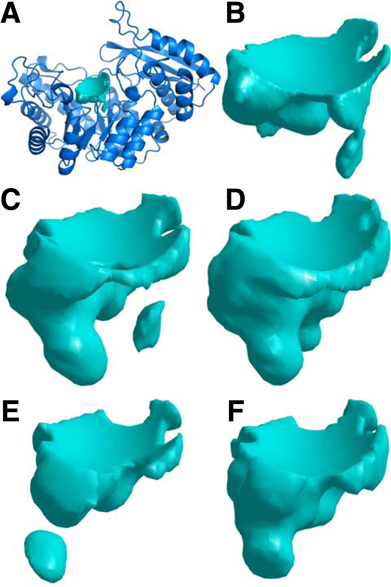
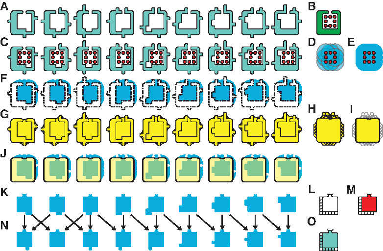
Conformational samples of the ligand binding cavity in yeast enolase (pdb: 1ebh). (A) The position of the cavity (teal) within the tertiary structure of enolase (blue cartoon). (B) The ligand binding cavity in the original crystal structure. (C–F) Binding cavities from other conformational samples of yeast enolase. All panels illustrate the cavity from the same perspective, generated with the global envelope surface, as described earlier.

3. Results

3.1. Sampled conformations vary significantly

Figure 4 illustrates conformational samples of the ligand binding cavity of yeast enolase (pdb: 1ebh). Each sample was aligned against the original PDB structure, and is shown from the same orientation. It is evident that smaller backbone and sidechain motions created substantial variations that changed the geometry of the cavity. The degree of variation exhibited in Figure 4 was not the most variable, relative to other cavities in the data set, nor was it the most conserved. Binding cavities in some proteins, such as atlantic salmon pancreatic elastase (pdb: 1elt), varied much more, while others varied less.

To further illustrate the degree of structural variation between ligand binding cavities, we plotted the volume of binding cavities in conformational samples of the entire dataset in Figure 5. The volume of trypsin cavities ranged from 248Å³ to 692Å³, the volume of chymotrypsin cavities ranged from 276Å³ to 568Å³, and elastase cavities ranged from 126Å³ to 552Å³, despite the general principle that chymotrypsin S1 cavities are larger to accommodate aromatic sidechains, and elastase cavities are smaller to accommodate amino acids like alanine or valine. The binding cavities of the enolase superfamily also exhibited substantial variation: Conformational samples of enolase cavities ranged from 90Å³ to 507Å³, mandelate racemases ranged from 225Å³ to 673Å³, and cavities sampled from muconate lactonizing enzyme were between 89Å³ and 343Å³. The substantial variation that can be observed between cavities illustrates the fundamental difficulty of accurately comparing binding site geometry in the presence of flexibility. Even though the variations are very small from the perspective of whole proteins, their effect on binding cavity geometry is substantial.

FIG. 5.

Volume of cavity sizes observed in conformational samples of serine proteases (A) and enolases (B), shown in red bars. Lines plot the quantity and spatial volume of cavities sampled for specific families.

Using VASP-S (Chen and Bandyopadhyay, 2011), we trained a statistical model of structural variation between trypsin binding cavities and a second model of variation between enolase binding cavities. Using these two models, we evaluated the statistical significance of volumetric differences between pairs of trypsin cavities and between pairs of enolase cavities. Over 65 percent of CSG differences were incorrectly classified by VASP-S as being so large as to be consistent with different binding preferences.

These data indicate that conformational flexibility creates substantial variations between different conformational samples of the same protein. For this reason, it is apparent that similarities and variations in individual conformational samples can mislead comparisons and that techniques like FAVA, which compensate for conformational variation, are essential for cavity comparison.

3.2. UPGMA clustering on frequent regions

A UPGMA clustering of frequent regions from the serine protease superfamily is plotted in Figure 6a. Trypsins were clustered tightly together, and elastases were correctly separated from trypsins, but Atlantic salmon elastase was placed as an outlier because it has zero volume. Chymotrypsin was separated, correctly, from both trypsins and elastases. In comparison, Figure 6b illustrates one example of a UPGMA clustering generated from randomly selected conformational samples of each protein. While trypsins were correctly clustered together, salmon elastase (pdb: 1elt) was incorrectly classified as being more similar to the trypsins than it was to porcine elastase (pdb: 1b0e), and porcine elastase was incorrectly clustered with chymotrypsin.

FIG. 6.

Comparison of clusterings of frequent regions and of individual cavities from serine protease structures. (A) Clustering of frequent regions. (B) Clustering of cavities from individual conformational samples. In both trees, topology is calculated based on volumetric distance. Coloring, which is independent of clustering topology, indicates the ligand binding preference of the protein.

Figure 8a illustrates a UPGMA clustering of frequent regions derived from enolase binding cavities. Frequent regions derived from muconate lactonizing enyzymes and enolases were separated correctly, as were frequent regions from mandelate racemase, with one exception: Mandelate racemase from Pseudomonas putida (pdb: 1mdr) was clustered with yeast enolase instead of with the other mandelate racemase from Zymomonas mobilis (pdb: 2ox4). A second UPGMA clustering, Figure 8b, was generated based on randomly selected conformational samples of each enolase superfamily structure. Individual conformational samples from the mandelate racemases in our dataset were distantly separated, indicating that their binding sites were quite different in these samples. Substantial differences were also apparent in baker's yeast enolase (pdb: 1ebh), which was separated from the enolase structures. Together, these results demonstrate that UPGMA clusterings of frequent regions represented similarities and differences in specificity. Overall, the flexible representation of binding cavities generated by FAVA exhibits fewer classification errors caused by conformational flexibility.

FIG. 8.

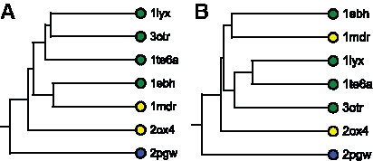
Comparison of clusterings of frequent regions and of individual cavities from enolase structures. (A) Clustering of frequent regions. (B) Clustering of cavities from individual conformational samples. In both trees, topology is calculated based on volumetric distance. Coloring, which is independent of clustering topology, indicates the ligand binding preference of the protein.

3.3. Influential amino acids

Differences in binding specificity can be caused by variations in the amino acids that surround the binding cavity, but these crucial variations can be obscured by sidechain and backbone motions. We hypothesized that amino acids that contribute to frequent differences between binding cavities, as opposed to those that create infrequent differences as a result of incidental motion, might also be responsible for differences in specificity. To evaluate this hypothesis, we computed the intersection volume between all residues r in all elastase structures (A), and all nonelastase serine protease cavities (B).

For example, the left of Figure 7 plots the degree of intersection between all conformational samples of all amino acids of porcine elastase (pdb: 1b0e) and binding cavities from conformational samples of salmon trypsin (pdb: 1bzx). Naturally, the vast majority of amino acids exhibited zero or very small intersection with the trypsin binding cavity because they are distant from the cavity when the two proteins are superposed. Two notable exceptions stand out: Samples of valine 216 and threonine 226 exhibited a median intersection volume of 45Å³ and 29Å³, respectively, with the conformational samples of the trypsin cavities. These amino acids are also known to block parts of the S1 pocket (inset, Fig. 7), shortening it to accommodate small hydrophobic residues (Shotton and Watson, 1970). In this example, FAVA identified sterically influential elastase residues that have an established role in specificity.

FIG. 7.

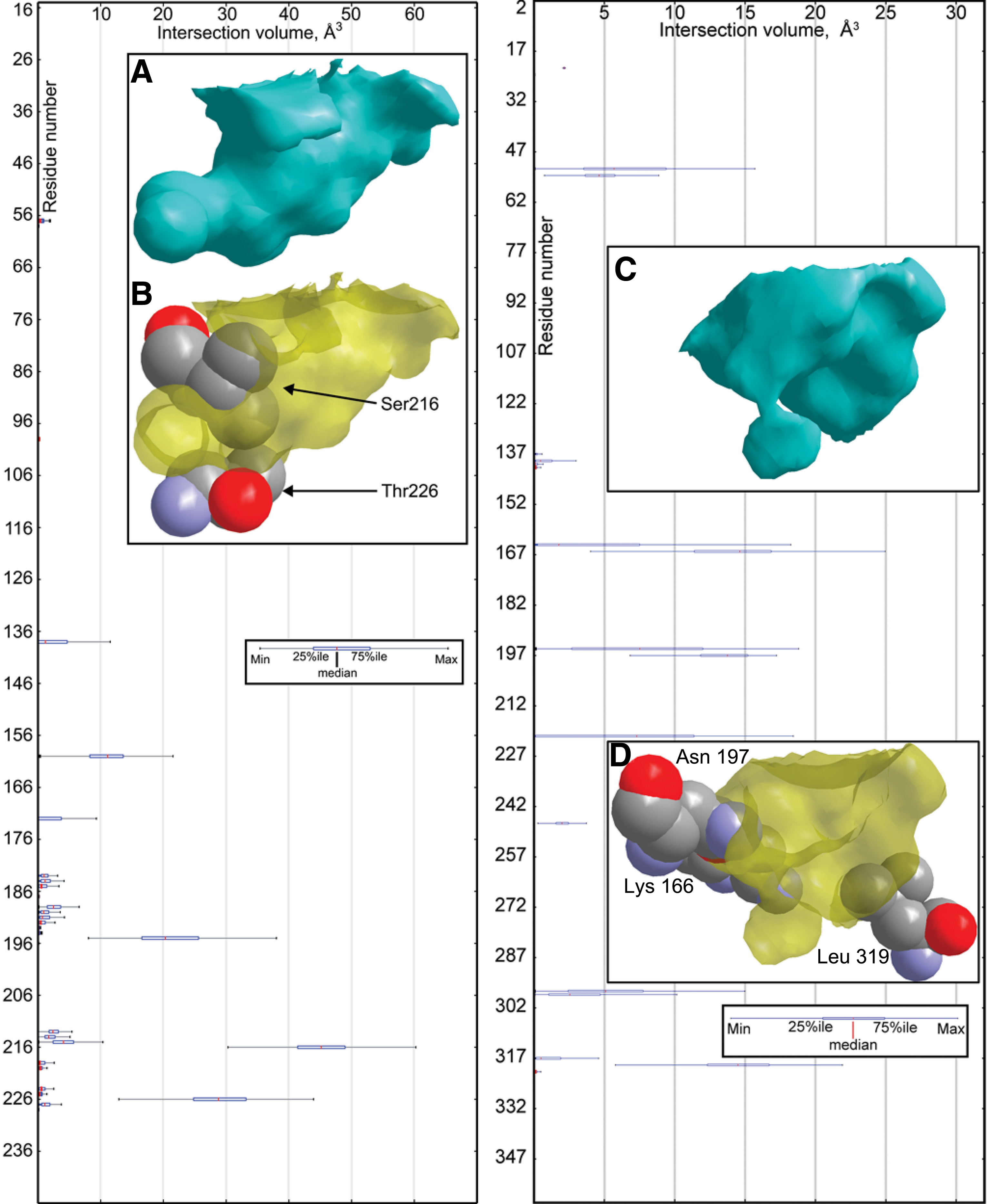
(Left), A plot of the intersection volume of amino acids from conformational samples of porcine pancreatic elastase (pdb: 1b0e) with cavities from conformational samples of salmon trypsin (pdb: 1bzx). (A) The trypsin cavity (teal). (B) One snapshot of Val216 and Thr226 from 1b0e, relative to the cavity. (Right), A plot of the intersection volume of amino acids from conformational samples of pseudomonas putida mandelate racemase (pdb: 1mdr) with cavities from conformational samples of saccharomyces cerevisiae enolase (pdb: 1ebh). (C) The enolase cavity (teal). (D) One snapshot of Lys166, Asp197, and Leu319 from 1mdr, relative to the cavity.

We observed similar findings among the binding sites of the enolase superfamily (Fig. 7, right). The aggregate intersection of conformational samples of amino acids from pseudomonas putida mandelate racemase (pdb: 1mdr) and binding cavities of saccharomyces cerevisiae enolase (pdb: 1ebh) offer a representative example: The vast majority of amino acids exhibited zero or very small intersection with the enolase binding cavity, but three exceptions are apparent: Samples of lysine 166, asparagine 197, and leucine 319 exhibited median intersection volumes of 14Å³, 13Å³, and 14Å³, respectively, with the conformational samples of the enolase cavities. Lysine 166 is believed to deprotonate (S)-mandelate substrates (Landro et al., 1994), asparagine 197 stabilizes the transition state (St. Maurice and Bearne, 2000), and leucine 319 assists in applying steric constraints in a hydrophobic pocket in the binding site (St. Maurice and Bearne, 2004). Here, FAVA identified influential mandelate racemase residues that have an established role in function and specificity.

To calibrate the significance of these intersection volumes, we measured the volume of structural differences created by the motions of amino acids with binding cavities from the same protein. While side chain motion creates small variations, aggregate differences were considerably smaller. For example, among amino acids of porcine pancreatic elastase (pdb: 1b0e), the amino acid that most intersects the binding cavity of 1b0e is serine 195, the nucleophilic serine responsible for catalysis in all serine proteases (Schechter and Berger, 1967). It occupies an median of 5Å³ inside samples of binding cavities in 1b0e. This result suggests that the motions observed in the amino acids of the serine protease and enolase superfamilies create differences in binding site geometry that were far more significant than those that occur normally.

4. Discussion

We have presented FAVA, a method for incorporating conformational variations into the geometric comparison of protein binding cavities. Whereas existing representations describe large conformational changes in order to discover remote homologs in different conformations, FAVA is designed for the detailed comparison of local features, such as ligand binding cavities, in spite of interference from small molecular motions, such as side chain flexibility. Whereas existing methods explicitly represent flexible regions of molecular structure, FAVA compiles volumetric representations of binding sites into frequent regions, which exclude infrequently occurring conformations and allow local conformational trends to emerge.

These conformational trends reflected differences in ligand binding preferences that could be obscured by conformational variation. A comparison of frequent regions generated from three subfamilies in each of the serine protease superfamily and the enolase superfamily revealed consistent variations in conformational trends that corresponded to differences in ligand binding preferences. If random conformational samples were compared instead of frequent regions, the resulting classification of binding sites could differ from actual binding preferences. Where conformational samples are selected arbitrarily, these results demonstrate the potential for errors in binding site comparison. Instead, using FAVA, we can mitigate these issues by classifying trends in a large sample of conformations.

Conformational trends also provided useful insights into the role of specific amino acids. We examined the range of conformations adopted by an amino acid over 100 nanoseconds and observed how frequently it would cause the binding site of a different protein to differ from its own. Amino acids that frequently cause differences in binding cavities almost always played a steric role in achieving binding specificity. While these influential residues occasionally move in ways that make different binding sites appear similar, their typical shape trends toward differences in binding sites, as might be expected based on different binding preferences. These results demonstrate that a detailed examination of many conformational samples can reveal individual influences on specificity and not simply trends in binding cavity shape.

FAVA has considerable potential for wider applications. First, it can be used with many sources of conformational samples, and as such it can provide insights into the patterns of conformational variations generated by many existing methods. As our capability to simulate molecular conformations continues to expand (Shaw et al., 2010; Beberg et al., 2009), larger and more representative samples will enhance the accuracy of comaparisons made with FAVA. Second, in many cases, efforts to create proteins with engineered binding preferences already involve the simulation of protein structures. FAVA provides an analysis of the resulting simulation data that can contribute insights into the roles of individual amino acids. By using conformational samples to examine the detailed motions of ligand binding sites, sampled representations can offer important tools for the analysis of ligand binding specificity.

Footnotes

Acknowledgment

This work was supported in part by National Science Foundation Grant 1320137 to Brian Chen and Katya Scheinberg.

Authors' Contributions

Z.G. and B.Y.C. conceived the algorithm proposed here, as well as the experimental design and analysis strategy, and carried out data analysis. Z.G. implemented the algorithm and performed production runs. B.Y.C. wrote the article.

Author Disclosure Statement

The authors declare that no competing financial interests exist.

References

Babbitt

P.C.

, Hasson

M.S.

, Wedekind

J.E.

, et al. 1996. The enolase superfamily: A general strategy for enzyme-catalyzed abstraction of the alpha-protons of carboxylic acids. Biochemistry, 35, 16489–16501.

Beberg

A.L.

, Ensign

D.L.

, Jayachandran

, et al. 2009. Folding@ home: Lessons from eight years of volunteer distributed computing. IEEE International Symposium on Parallel & Distributed Processing, 2009. IPDPS 2009, IEEE, pp. 1–8.

Berendsen

, Postma

, van Gunsteren

, and Hermans

1981. Intermolecular Forces. Reidel Publishing Company, Dordrecht.

Berglund

, Smalas

, Outzen

, and Willassen

1998. Purification and characterization of pancreatic elastase from North Atlantic salmon (Salmo salar). Mol. Mar. Biol. Biotechnol., 7, 105–114.

Berman

H.M.

, Westbrook

, Feng

, et al. 2000. The Protein Data Bank. Nucleic Acids Res. 28, 235–242.

Binkowski

T.A.

, Freeman

, and Liang

2004. pvSOAR: Detecting similar surface patterns of pocket and void surfaces of amino acid residues on proteins. Nucleic Acids Res. 32, W555–W558.

Birzele

, Gewehr

J.E.

, Csaba

, and Zimmer

2007. Vorolign—fast structural alignment using voronoi contacts. Bioinformatics, 23, e205–e211.

Bryant

D.H.

, Moll

, Finn

P.W.

, and Kavraki

L.E.

2013. Combinatorial clustering of residue position subsets predicts inhibitor affinity across the human kinome. PLoS Comput. Biol., 9, e1003087.

Chen

, and Bandyopadhyay

2011. VASP-S: A volumetric analysis and statistical model for predicting steric influences on protein-ligand binding specificity. Proceedings of 2011 IEEE International Conference on Bioinformatics and Biomedicine, IEEE, pp. 22–29.

10.

Chen

B.Y.

, and Honig

2010. VASP: A volumetric analysis of surface properties yields insights into protein-ligand binding specificity. PLoS Comput. Biol., 6, 11.

11.

Chen

B.Y.

, Fofanov

V.Y.

, Bryant

D.H.

, et al. 2007. The MASH pipeline for protein function prediction and an algorithm for the geometric refinement of 3D motifs. J. Comp. Biol., 14, 791–816.

12.

Chen

B.Y.

, Fofanov

V.Y.

, Kristensen

D.M.

, et al. 2005. Algorithms for structural comparison and statistical analysis of 3D protein motifs. Pac. Symp. Biocomput., 345, 334–345.

13.

Connolly

1983. Solvent-accessible surfaces of proteins and nucleic acids. Science, 221, 709–713.

14.

DeLano

W.L.

2002. The PyMOL Molecular Graphics System. DeLano Scientific, San Carlos, CA.

15.

Dundas

, Adamian

, and Liang

2011. Structural signatures of enzyme binding pockets from order-independent surface alignment: A study of metalloendopeptidase and nad binding proteins. J. Mol. Biol., 406, 713–729.

16.

Felsenstein

1989. Phylip—phylogeny inference package (version 3.2). Cladistics, 5, 163–166.

17.

Godshall

B.G.

, and Chen

B.Y.

2012. Improving accuracy in binding site comparison with homology modeling. IEEE International Conference on Bioinformatics and Biomedicine Workshops (BIBMW), 2012, IEEE, pp. 662–669.

18.

Godshall

B.G.

, Tang

, Yang

, and Chen

B.Y.

2013. An aggregate analysis of many predicted structures to reduce errors in protein structure comparison caused by conformational flexibility. BMC Struct. Biol., 13, S10.

19.

Gráf

, Jancsó

, Szilágyi

, et al. 1988. Electrostatic complementarity within the substrate-binding pocket of trypsin. Proc. Natl. Acad. Sci. USA, 85, 4961–4965.

20.

Gunasekaran

, and Nussinov

2007. How different are structurally flexible and rigid binding sites? Sequence and structural features discriminating proteins that do and do not undergo conformational change upon ligand binding. J. Mol. Biol., 365, 257–273.

21.

Guo

, and Chen

B.Y.

2014. Variational bayesian clustering on protein cavity conformations for detecting influential amino acids. Proceedings of the 5th ACM Conference on Bioinformatics, Computational Biology, and Health Informatics, ACM, pp. 703–710.

22.

Guo

, Kuhlengel

, Stinson

, et al. 2014. A flexible volumetric comparison of protein cavities can reveal patterns in ligand binding specificity. Proceedings of the 5th ACM Conference on Bioinformatics, Computational Biology, and Health Informatics, ACM, pp. 445–454.

23.

Hess

2008. P-LINCS: A parallel linear constraint solver for molecular simulation. J. Chem. Theory Comput., 4, 116–122.

24.

Hess

, Kutzner

, van der Spoel

, and Lindahl

2008. GROMACS 4: Algorithms for highly efficient, load-balanced, and scalable molecular simulation. J. Chem. Theory Comput., 4, 435–447.

25.

Holm

, and Sander

1994. The fssp database of structurally aligned protein fold families. Nucleic Acids Res., 22, 3600.

26.

Holm

, and Sander

1996. Mapping the protein universe. Science, 273, 595–603.

27.

Jorgensen

W.L.

, Chandrasekhar

, Madura

J.D.

, et al. 1983. Comparison of simple potential functions for simulating liquid water. J. Chem. Phys., 79, 926–935.

28.

Junier

, and Zdobnov

E.M.

2010. The newick utilities: High-throughput phylogenetic tree processing in the unix shell. Bioinformatics, 26, 1669–1670.

29.

Konc

, and Janežič

2010. Probis algorithm for detection of structurally similar protein binding sites by local structural alignment. Bioinformatics, 26, 1160–1168.

30.

Kühnel

, and Luisi

B.F.

2001. Crystal structure of the Escherichia coli RNA degradosome component enolase. J. Mol. Biol., 313, 583–592.

31.

Landro

J.A.

, Gerlt

J.A.

, Kozarich

J.W.

, et al. 1994. The role of lysine 166 in the mechanism of mandelate racemase from pseudomonas putida: Mechanistic and crystallographic evidence for stereospecific alkylation by (r)-. alpha.-phenylglycidate. Biochemistry, 33, 635–643.

32.

Menke

, Berger

, and Cowen

2008. Matt: Local flexibility aids protein multiple structure alignment. PLoS Comput. Biol., 4, e10.

33.

Morihara

, and Tsuzuki

1969. Comparison of the specificities of various serine proteinases from microorganisms. Arch. Biochem. Biophys., 129, 620–634.

34.

Mosca

, and Schneider

T.R.

2008. Rapido: A web server for the alignment of protein structures in the presence of conformational changes. Nucleic Acids Res., 36, W42–W46.

35.

Murzin

a.G.

, Brenner

S.E.

, Hubbard

, and Chothia

1995. SCOP: A structural classification of proteins database for the investigation of sequences and structures. J. Mol. Biol., 247, 536–540.

36.

Nose

, and Klein

1983. Constant pressure molecular dynamics for molecular systems. Mol. Phys., 50, 1055–1076.

37.

Nussinov

, and Wolfson

H.J.

1991. Efficient detection of three-dimensional structural motifs in biological macromolecules by computer vision techniques. Proc. Natl. Acad. Sci. USA, 88, 10495–10499.

38.

Olson

, and Shehu

2012. Evolutionary-inspired probabilistic search for enhancing sampling of local minima in the protein energy surface. Proteome Sci., 10, S5.

39.

Orengo

C.A.

, and Taylor

W.R.

1996. SSAP: Sequential Structure Alignment Program for protein structure comparison. Method Enzymol., 266, 617–635.

40.

Orengo

C.A.

, Michie

a.D.

, Jones

, et al. 1997. CATH—a hierarchic classification of protein domain structures. Structure., 5, 1093–1108.

41.

Parrinello

, and Rahman

1981. Polymorphic transitions in single crystals: A new molecular dynamics method. J. Appl. Phys., 52, 7182.

42.

Petrey

, and Honig

2003. GRASP2: Visualization, surface properties, and electrostatics of macromolecular structures and sequences. Method Enzymol. 374, 492–509.

43.

Rakus

J.F.

, Fedorov

A.A.

, Fedorov

E.V.

, et al. 2008. Evolution of enzymatic activities in the enolase superfamily: L-rhamnonate dehydratase. Biochemistry, 47, 9944–9954.

44.

Russell

R.B.

1998. Detection of protein three-dimensional side-chain patterns: New examples of convergent evolution. J. Mol. Biol., 279, 1211–1227.

45.

Schaer

, and Stone

1991. Face traverses and a volume algorithm for polyhedra. Lect. Notes Comput. Sci., 555/1991, 290–297.

46.

Schafer

S.L.

, Barrett

W.C.

, Kallarakal

A.T.

, et al. 1996. Mechanism of the reaction catalyzed by mandelate racemase: Structure and mechanistic properties of the D270N mutant. Biochemistry, 35, 5662–5669.

47.

Schechter

, and Berger

1967. On the size of the active site in proteases. I. Papain. Biochem. Biophys. Res. Commun., 27, 157–162.

48.

Shatsky

, Nussinov

, and Wolfson

H.J.

2004. FlexProt: Alignment of flexible protein structures without a predefinition of hinge regions. J. Comput. Biol., 11, 83–106.

49.

Shaw

D.E.

, Maragakis

, Lindorff-Larsen

, et al. 2010. Atomic-level characterization of the structural dynamics of proteins. Science, 330, 341–346.

50.

Shindyalov

I.N.

, and Bourne

P.E.

1998. Protein structure alignment by incremental combinatorial extension (CE) of the optimal path. Protein Eng. 11, 739–747.

51.

Shotton

, and Watson

1970. Three-dimensional structure of tosyl-elastase. Nature, 225, 811–816.

52.

Sneath

P.H.

, and Sokal

R.R.

1973. Numerical Taxonomy. The Principles and Practice of Numerical Classification. W.H. Freeman, New York.

53.

St. Maurice

, and Bearne

S.L.

2000. Reaction intermediate analogues for mandelate racemase: Interaction between asn 197 and the α-hydroxyl of the substrate promotes catalysis. Biochemistry, 39, 13324–13335.

54.

St. Maurice

, and Bearne

S.L.

2004. Hydrophobic nature of the active site of mandelate racemase. Biochemistry, 43, 2524–2532.

55.

Stark

, Sunyaev

, and Russell

R.B.

2003. A model for statistical significance of local similarities in structure. J. Mol. Biol., 326, 1307–1316.

56.

Umeyama

1991. Least-squares estimation of transformation parameters between two point patterns. IEEE Trans. Pattern Anal. Mach. Intell., 13, 376–380.

57.

Vesterstrøm

, and Taylor

W.R.

2006. Flexible secondary structure based protein structure comparison applied to the detection of circular permutation. J. Comput. Biol., 13, 43–63.

58.

Yang

A.-S.

, and Honig

2000. An integrated approach to the analysis and modeling of protein sequences and structures. I. Protein structural alignment and a quantitative measure for protein structural distance. J. Mol. Biol., 301, 665–678.

59.

, and Godzik

2005. Multiple flexible structure alignment using partial order graphs. Bioinformatics, 21, 2362–2369.

60.

Zhang

, and Skolnick

2005. Tm-align: A protein structure alignment algorithm based on the tm-score. Nucleic Acids Res., 33, 2302–2309.