Metagenomic Classification Using an Abstraction Augmented Markov Model

Abstract

The abstraction augmented Markov model (AAMM) is an extension of a Markov model that can be used for the analysis of genetic sequences. It is developed using the frequencies of all possible consecutive words with same length (p-mers). This article will review the theory behind AAMM and apply the theory behind AAMM in metagenomic classification.

1. Introduction

Sequence analysis refers to the process of examining a DNA, RNA, or protein sequence to investigate its characteristics, structure, function, or etiology. This field has grown enormously in recent years due to the dramatic increase in sequence data, driven by the completion of a draft human genome in 2001 (Consortium, 2001). Further research on the HGP and the growth of next generation sequencing (NGS) technologies has led to a digital tsunami of sequencing data (Fuhrman, 2012). Metagenomics, the study of genetic material recovered directly from environmental samples (Hugenholtz et al., 1998), is one field born from the increasing accessibility and affordability of NGS technologies. One example of such a project is the Human Microbiome Project (Turnbaugh et al., 2007), whose goal is to characterize the taxonomic diversity of microbial communities within the human body. Once sequences within an environment are characterized, it is hoped that they can be classified into known phylogenetic categories in order to infer their representative organism's function within the sampled environment. One can view this problem as a classification problem, in which the metagenomic data is used to create a model for the organisms within the sample, and then new organisms can be classified into this model (or not). Often, 16S ribosomal (16S rRNA) is used for phylogenetic studies since it is highly conserved between different species of bacteria and archaea (Case et al., 2007). Also, 16S rRNA is a component of the 30S small subunit of prokaryotic ribosomes and consists of 1562 nucleotides, on average (Weisburg et al., 1991).

Once the NGS data are available, most metagenomic data analyses proceed in the identification of short reads by aligning sequences within the sample to their closest relatives using reference databases containing full-length sequences (Kim et al., 2013). BLAST (Altschul et al., 1990) is a popular choice for organism classification, and often the top hits from BLAST results are used to identify the taxa of query sequences. However, since reads from metagenomic data are often short DNA fragments, the top hits are not always accurate. Furthermore, the computational load for alignment-based schema increases as a power function with the length of the sequences, which makes it infeasible to search large genetic databases (Zhu, 2014). Other algorithms, such as MEGAN (Huson et al., 2007) and TANGO (Clemente et al., 2011), improve speed and accuracy in taxonomic classification by using BLAST in conjunction with other consensus measures. A naive Bayesian classifier implemented in the Ribosomal Database Project [RDP, Wang et al. (2007)] is very computationally efficient, as it trains sequences using only eight-word alignments. It further gives a probability of a correct assignment along with bootstrapped confidence intervals. While all of the previously mentioned algorithms have produced meaningful results, the algorithms rely on alignment of sequences that may arise from heretofore unknown and unsequenced organisms. As a result of this lack of information, and for the sake of computational efficiency, many researchers have developed so-called “alignment-free” algorithms.

Alignment-free methods to compare biological sequences were first proposed by Blaisdell (Blaisdell, 1986, 1989). Since that time, the pace of development and improvement for alignment-free methods has increased dramatically. There are two main categories of proposed methods: methods based on word (nucleotides/amino acids) counts, and those that are not based on fixed word-length segments. As for the methods in the first group, sequence similarity is measured using procedures based on metrics defined in coordinate space on word-count vectors. Such metrics include Euclidean or Mahalanobis distance (Torney et al., 1990; Hide et al., 1994; Wu et al., 2001) and correlation/covariance methods (Fichant and Gautier, 1987; Gibbs et al., 1971; Solovyev and Makarova, 1993; van Heel, 1991). Other methods do not involve counting the frequency of segments with fixed length, rather, these algorithms use methods from information theory (Wu et al., 1997), Kolmorgorov complexity theory (Li et al., 2001), angle metrics (Stuart et al., 2002), and iterative maps (Almeida and Vinga, 2002).

Alignment-free methods provide a computationally efficient way to overcome the shortcomings of traditional alignment-based methods. However, important sequence structural information is sacrificed (Zhu, 2014). Markov models, in particular Hidden Markov Models (HMMs), provide a scheme for maintaining structure within the sequence (Yoon, 2009). The Markov structure specifies that the probability of observing a particular nucleotide in a sequence depends only on the previous nucleotide. Methods for sequence classification using HMMs typically rely on alignment to a reference sequence. Additionally, HMM algorithms often require long sequences in order to incorporate long-term sequence dependency. Long sequences are not always available in metagenomic data. Furthermore, HMMs require user specification of several parameters that, if misspecified, could produce misleading results (Kotamarti et al., 2010).

There are other Markov-based sequence classification methods that have been shown to model sequence structure, exhibit computational efficiency, and do not need alignment. One such method is “quasi-alignment,” which is based on the extensible Markov model (Dunham et al., 2004), extended to biological sequence analysis (Hahsler and Nagar, 2014; Kotamarti et al., 2010). Quasi-alignment consists of three standard steps: preprocessing sequences, learning target EMMs, and scoring query sequences against target EMMs. In the context of metagenomics, one can construct an EMM using sequences of the same phylogenetic class from a well-known database, such as Greengenes (DeSantis et al., 2008). An example of an EMM constructed from the 302 metagenomic 16S rRNA sequences for the genus Escherischia is shown in chapter 1 of Zhu (2014). Each EMM represents one taxon at a particular phylogenetic rank. When an unknown sequence is to be classified, it is scored against all the EMMs at the specified rank and is assigned to the class with the highest score. Details of the scoring process are given in chapter 2 of Zhu (2014) and summarized in Kotamarti et al. (2010). The method is implemented in the R package QuasiAlign (Hahsler and Nagar, 2014). In this way, one can assign sequences within any environmental sample without having to align the sequences against a reference database. Instead, the query sequences can be quasi-aligned against an EMM that represents an entire phylogenetic taxon. Quasi-alignment has been shown to outperform naive Bayes, as implemented in RDP, by a large margin (Nagar, 2013). In addition, quasi-alignment can provide an accurate classification at the genus and species level, which is not possible for other methods due to the small intra-sequence variability at such levels.

Another Markov-based model is the abstraction augmented Markov model (AAMM). Like quasi-alignment, it is a computationally efficient method that does not require alignment of query sequences to a target sequence database. As a result, neither method is affected by minor sequencing errors or multiple sequence alignment errors. AAMMs effectively reduce the number of numeric parameters of a standard Markov model through abstraction, or the grouping of strings of length p into hierarchical clusters (Caragea et al., 2009). In AAMMs, the abstraction acts as a regularizer that helps minimize overfitting when the training sequence set is limited in size. Therefore, AAMMs can perform much more robustly than an HMM (Caragea, 2009). Previously, AAMMs have been evaluated on three protein subcellular localization prediction tasks (Caragea, 2009). It was shown that AAMMs are able to use significantly smaller number of features than traditional higher order Markov models and perform significantly better than variable Markov models. AAMMs have a theoretical advantage over the EMMs used in quasi-alignment, in that the base model for an AAMM does indeed have the Markov property (Caragea, 2009). Even though EMMs as originally defined are Markov (Dunham et al., 2004), when applying EMM in quasi-alignment, the Markov property is no longer tenable. In quasi-alignment, each state represents a cluster of NSVs that are created from overlapping gene sequence segments of length p. These states cannot be specified prior to creating the model, and the NSV's within the states are not statistically independent (Zhu, 2014).

The purpose of this article is to present the AAMM as a method of metagenomic analysis that carries the theoretical properties of Markov models while retaining the efficiency of alignment-free methods. The formal definition of an AAMM and an algorithm for obtaining the abstractions are presented in section 2. Details of the implementation are in section 3, where we also show that AAMMs are able to classify correctly approximately 95% of sequences to their appropriate taxa, even at the genus level. Finally, we discuss future developments and applications in section 4.

2. Methods

Abstraction augmented Markov models have been evaluated on three protein subcellular localization prediction tasks (Caragea, 2009), where it was shown that AAMMs were able to use a significantly smaller number of parameters than traditional higher order Markov models, and perform significantly better in predictive accuracy than variable Markov models. AAMMs are able to reduce the number of numeric parameters of higher order Markov models through successively grouping all possible consecutive words of length p according to the word frequencies in training data set. When constructing an AAMM, a set of all existing p-mers in the training data set is clustered into an abstraction hierarchy according to some similarity measure of p-mer frequencies. This section gives formal definitions and explains the theory behind the AAMM.

2.1. Definitions

An abstraction hierarchy is a rooted tree model whose root represents a set of all existing p-mers, while each leaf-node represents one individual p-mer. Formally,

Definition 1. An abstraction hierarchy \documentclass{aastex}\usepackage{amsbsy}\usepackage{amsfonts}\usepackage{amssymb}\usepackage{bm}\usepackage{mathrsfs}\usepackage{pifont}\usepackage{stmaryrd}\usepackage{textcomp}\usepackage{portland, xspace}\usepackage{amsmath, amsxtra}\pagestyle{empty}\DeclareMathSizes{10}{9}{7}{6}\begin{document} $${ \cal T}$$ \end{document} over a set of p-mers \documentclass{aastex}\usepackage{amsbsy}\usepackage{amsfonts}\usepackage{amssymb}\usepackage{bm}\usepackage{mathrsfs}\usepackage{pifont}\usepackage{stmaryrd}\usepackage{textcomp}\usepackage{portland, xspace}\usepackage{amsmath, amsxtra}\pagestyle{empty}\DeclareMathSizes{10}{9}{7}{6}\begin{document} $${ \cal S}$$ \end{document} is a rooted tree such that

• The root of \documentclass{aastex}\usepackage{amsbsy}\usepackage{amsfonts}\usepackage{amssymb}\usepackage{bm}\usepackage{mathrsfs}\usepackage{pifont}\usepackage{stmaryrd}\usepackage{textcomp}\usepackage{portland, xspace}\usepackage{amsmath, amsxtra}\pagestyle{empty}\DeclareMathSizes{10}{9}{7}{6}\begin{document} $${\cal T}$$ \end{document} denotes \documentclass{aastex}\usepackage{amsbsy}\usepackage{amsfonts}\usepackage{amssymb}\usepackage{bm}\usepackage{mathrsfs}\usepackage{pifont}\usepackage{stmaryrd}\usepackage{textcomp}\usepackage{portland, xspace}\usepackage{amsmath, amsxtra}\pagestyle{empty}\DeclareMathSizes{10}{9}{7}{6}\begin{document} $${ \cal S}$$ \end{document}

• The leaves of \documentclass{aastex}\usepackage{amsbsy}\usepackage{amsfonts}\usepackage{amssymb}\usepackage{bm}\usepackage{mathrsfs}\usepackage{pifont}\usepackage{stmaryrd}\usepackage{textcomp}\usepackage{portland, xspace}\usepackage{amsmath, amsxtra}\pagestyle{empty}\DeclareMathSizes{10}{9}{7}{6}\begin{document} $${ \cal T}$$ \end{document} correspond to singleton sets containing individual p-mers in \documentclass{aastex}\usepackage{amsbsy}\usepackage{amsfonts}\usepackage{amssymb}\usepackage{bm}\usepackage{mathrsfs}\usepackage{pifont}\usepackage{stmaryrd}\usepackage{textcomp}\usepackage{portland, xspace}\usepackage{amsmath, amsxtra}\pagestyle{empty}\DeclareMathSizes{10}{9}{7}{6}\begin{document} $${ \cal S}$$ \end{document}

• The children of each node {a₁,…,a_m} ∈ \documentclass{aastex}\usepackage{amsbsy}\usepackage{amsfonts}\usepackage{amssymb}\usepackage{bm}\usepackage{mathrsfs}\usepackage{pifont}\usepackage{stmaryrd}\usepackage{textcomp}\usepackage{portland, xspace}\usepackage{amsmath, amsxtra}\pagestyle{empty}\DeclareMathSizes{10}{9}{7}{6}\begin{document} $${ \cal A}$$ \end{document} correspond to a partition of the set of p-mers denoted by a_i. This partition is also called an abstraction.

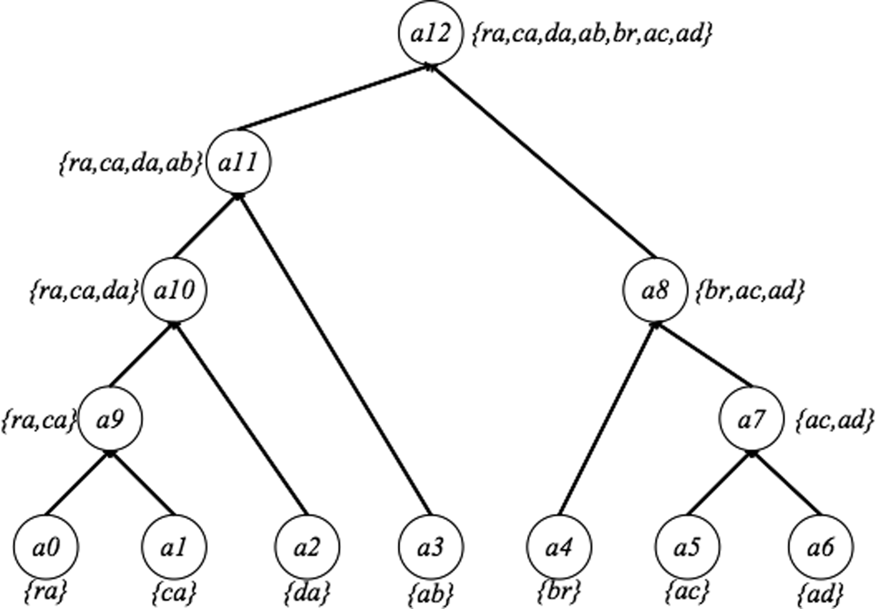
Figure 1 shows an example of abstraction hierarchy on a set \documentclass{aastex}\usepackage{amsbsy}\usepackage{amsfonts}\usepackage{amssymb}\usepackage{bm}\usepackage{mathrsfs}\usepackage{pifont}\usepackage{stmaryrd}\usepackage{textcomp}\usepackage{portland, xspace}\usepackage{amsmath, amsxtra}\pagestyle{empty}\DeclareMathSizes{10}{9}{7}{6}\begin{document} $${ \cal S}$$ \end{document} = {ra, ca, da, ab, br, ac, ad} of 2-mers over the alphabet {a, b, c, d, r}. This abstraction hierarchy is learned from the training sequence abracadabra.

FIG. 1.

An example of an abstraction hierarchy learned from the training sequence abracadabra. The root node (top) represents the entire set S, and the leaf nodes (bottom) indicate each individual 2-mer. Nodes are merged from the leaf to the root, forming abstraction hierarchies.

The root of the above abstraction hierarchy a₁₂ represents the entire set \documentclass{aastex}\usepackage{amsbsy}\usepackage{amsfonts}\usepackage{amssymb}\usepackage{bm}\usepackage{mathrsfs}\usepackage{pifont}\usepackage{stmaryrd}\usepackage{textcomp}\usepackage{portland, xspace}\usepackage{amsmath, amsxtra}\pagestyle{empty}\DeclareMathSizes{10}{9}{7}{6}\begin{document} $${ \cal S}$$ \end{document} . The leaf nodes {a₀,…,a₆} denote each individual 2-mer in the set \documentclass{aastex}\usepackage{amsbsy}\usepackage{amsfonts}\usepackage{amssymb}\usepackage{bm}\usepackage{mathrsfs}\usepackage{pifont}\usepackage{stmaryrd}\usepackage{textcomp}\usepackage{portland, xspace}\usepackage{amsmath, amsxtra}\pagestyle{empty}\DeclareMathSizes{10}{9}{7}{6}\begin{document} $${ \cal S}$$ \end{document} = {ra, ca, da, ab, br, ac, ad}. The children of each node correspond to an abstraction of the set of p-mers denoted by that node. For example, the children of a₁₂ are a₁₁ and a₈ in Figure 1; therefore, the set {ra,ca,da,ab} denoted by a₁₁ and set {br, ac, ad} denoted by a₈ compose a partition of \documentclass{aastex}\usepackage{amsbsy}\usepackage{amsfonts}\usepackage{amssymb}\usepackage{bm}\usepackage{mathrsfs}\usepackage{pifont}\usepackage{stmaryrd}\usepackage{textcomp}\usepackage{portland, xspace}\usepackage{amsmath, amsxtra}\pagestyle{empty}\DeclareMathSizes{10}{9}{7}{6}\begin{document} $${ \cal S}$$ \end{document} denoted by a₁₂. Different partitions of \documentclass{aastex}\usepackage{amsbsy}\usepackage{amsfonts}\usepackage{amssymb}\usepackage{bm}\usepackage{mathrsfs}\usepackage{pifont}\usepackage{stmaryrd}\usepackage{textcomp}\usepackage{portland, xspace}\usepackage{amsmath, amsxtra}\pagestyle{empty}\DeclareMathSizes{10}{9}{7}{6}\begin{document} $${ \cal S}$$ \end{document} specify different levels of this abstraction hierarchy, which leads to the concept of an m-Cut.

Definition 2. An m-cut of an abstraction hierarchy is a unique subset of m nodes of the abstraction hierarchy, which partitions the set of all possible p-mers into m non-overlapping subsets. In other words, an m-cut is the union of the sets of p-mers of the corresponding m nodes in set \documentclass{aastex}\usepackage{amsbsy}\usepackage{amsfonts}\usepackage{amssymb}\usepackage{bm}\usepackage{mathrsfs}\usepackage{pifont}\usepackage{stmaryrd}\usepackage{textcomp}\usepackage{portland, xspace}\usepackage{amsmath, amsxtra}\pagestyle{empty}\DeclareMathSizes{10}{9}{7}{6}\begin{document} $${ \cal S}$$ \end{document} .

Specifically, an m-cut γ_m partitions the set \documentclass{aastex}\usepackage{amsbsy}\usepackage{amsfonts}\usepackage{amssymb}\usepackage{bm}\usepackage{mathrsfs}\usepackage{pifont}\usepackage{stmaryrd}\usepackage{textcomp}\usepackage{portland, xspace}\usepackage{amsmath, amsxtra}\pagestyle{empty}\DeclareMathSizes{10}{9}{7}{6}\begin{document} $${ \cal S}$$ \end{document} into m non-overlapping subsets \documentclass{aastex}\usepackage{amsbsy}\usepackage{amsfonts}\usepackage{amssymb}\usepackage{bm}\usepackage{mathrsfs}\usepackage{pifont}\usepackage{stmaryrd}\usepackage{textcomp}\usepackage{portland, xspace}\usepackage{amsmath, amsxtra}\pagestyle{empty}\DeclareMathSizes{10}{9}{7}{6}\begin{document} $${ \cal A} = \{ a_1 : { \cal S}_1 , \ldots , a_m : { \cal S}_m \} ,$$ \end{document} where a_i represents the ith abstraction and \documentclass{aastex}\usepackage{amsbsy}\usepackage{amsfonts}\usepackage{amssymb}\usepackage{bm}\usepackage{mathrsfs}\usepackage{pifont}\usepackage{stmaryrd}\usepackage{textcomp}\usepackage{portland, xspace}\usepackage{amsmath, amsxtra}\pagestyle{empty}\DeclareMathSizes{10}{9}{7}{6}\begin{document} $${ \cal S}_i$$ \end{document} denotes the subset of p-mers, which are grouped together into the ith abstraction based on some similarity measure. For example, the two-cut of the abstraction hierarchy from Figure 1 is {a₁₁, a₈}. Node a₁₁ and a₈ partition the entire 2-mer set \documentclass{aastex}\usepackage{amsbsy}\usepackage{amsfonts}\usepackage{amssymb}\usepackage{bm}\usepackage{mathrsfs}\usepackage{pifont}\usepackage{stmaryrd}\usepackage{textcomp}\usepackage{portland, xspace}\usepackage{amsmath, amsxtra}\pagestyle{empty}\DeclareMathSizes{10}{9}{7}{6}\begin{document} $${ \cal S}$$ \end{document} = {ra, ca, da, ab,br, ac, ad} into two groups, {ra, ca, da, ab} and {br, ac, ad}. The three-cut of this abstraction hierarchy is {a₁₀, a₃, a₈}. A two-cut and a three-cut are depicted in Figure 2. A procedure for selecting the appropriate m-cut for a data set is given in section 2.3.

FIG. 2.

An example of a two-cut (a) and a three-cut (b) for the example abstraction hierarchy of the sequence abracadabra. The two-cut creates two non-overlapping trees from the original abstraction hierarchy, and the three-cut creates three non-overlapping trees. The root node for each cut is depicted as a solid circle.

AAMMs incorporate new variables \documentclass{aastex}\usepackage{amsbsy}\usepackage{amsfonts}\usepackage{amssymb}\usepackage{bm}\usepackage{mathrsfs}\usepackage{pifont}\usepackage{stmaryrd}\usepackage{textcomp}\usepackage{portland, xspace}\usepackage{amsmath, amsxtra}\pagestyle{empty}\DeclareMathSizes{10}{9}{7}{6}\begin{document} $$a_i \in { \cal A}$$ \end{document} , where \documentclass{aastex}\usepackage{amsbsy}\usepackage{amsfonts}\usepackage{amssymb}\usepackage{bm}\usepackage{mathrsfs}\usepackage{pifont}\usepackage{stmaryrd}\usepackage{textcomp}\usepackage{portland, xspace}\usepackage{amsmath, amsxtra}\pagestyle{empty}\DeclareMathSizes{10}{9}{7}{6}\begin{document} $${ \cal A}$$ \end{document} = {a₁,…,a_m} is a set of abstractions over the set of all p-mers \documentclass{aastex}\usepackage{amsbsy}\usepackage{amsfonts}\usepackage{amssymb}\usepackage{bm}\usepackage{mathrsfs}\usepackage{pifont}\usepackage{stmaryrd}\usepackage{textcomp}\usepackage{portland, xspace}\usepackage{amsmath, amsxtra}\pagestyle{empty}\DeclareMathSizes{10}{9}{7}{6}\begin{document} $${ \cal S}_{i - 1} ,$$ \end{document} for i = 1…,n − 1, and n is the total number of p-mers. Each node X_i in an AAMM directly depends on an abstraction a_i. The procedure for building AAMMs involves learning an abstraction hierarchy and estimating model parameters using the appropriate abstraction hierarchy. Once the abstraction hierarchy \documentclass{aastex}\usepackage{amsbsy}\usepackage{amsfonts}\usepackage{amssymb}\usepackage{bm}\usepackage{mathrsfs}\usepackage{pifont}\usepackage{stmaryrd}\usepackage{textcomp}\usepackage{portland, xspace}\usepackage{amsmath, amsxtra}\pagestyle{empty}\DeclareMathSizes{10}{9}{7}{6}\begin{document} $${ \cal A}$$ \end{document} is learned, a similarity measure is used to calculate the similarity between two abstractions. Then, abstractions are recursively grouped according to this similarity measure until all abstractions are part of the hierarchy. The learning algorithm is as follows:

1. Input a set of p-mers \documentclass{aastex}\usepackage{amsbsy}\usepackage{amsfonts}\usepackage{amssymb}\usepackage{bm}\usepackage{mathrsfs}\usepackage{pifont}\usepackage{stmaryrd}\usepackage{textcomp}\usepackage{portland, xspace}\usepackage{amsmath, amsxtra}\pagestyle{empty}\DeclareMathSizes{10}{9}{7}{6}\begin{document} $${ \cal S} = \{ s_1, \ldots ,s_n \} $$ \end{document} and training sequences \documentclass{aastex}\usepackage{amsbsy}\usepackage{amsfonts}\usepackage{amssymb}\usepackage{bm}\usepackage{mathrsfs}\usepackage{pifont}\usepackage{stmaryrd}\usepackage{textcomp}\usepackage{portland, xspace}\usepackage{amsmath, amsxtra}\pagestyle{empty}\DeclareMathSizes{10}{9}{7}{6}\begin{document} $${\cal D}$$ \end{document} .

2. Initialize \documentclass{aastex}\usepackage{amsbsy}\usepackage{amsfonts}\usepackage{amssymb}\usepackage{bm}\usepackage{mathrsfs}\usepackage{pifont}\usepackage{stmaryrd}\usepackage{textcomp}\usepackage{portland, xspace}\usepackage{amsmath, amsxtra}\pagestyle{empty}\DeclareMathSizes{10}{9}{7}{6}\begin{document} $${\cal A} = \{ a_1 \ : \ s_1 , \ldots , a_n \ : \ s_n \} $$ \end{document} and \documentclass{aastex}\usepackage{amsbsy}\usepackage{amsfonts}\usepackage{amssymb}\usepackage{bm}\usepackage{mathrsfs}\usepackage{pifont}\usepackage{stmaryrd}\usepackage{textcomp}\usepackage{portland, xspace}\usepackage{amsmath, amsxtra}\pagestyle{empty}\DeclareMathSizes{10}{9}{7}{6}\begin{document} $${ \cal T}= \{ a_1 \ : \ s_1 , \ldots , a_n \ : \ s_n \} $$ \end{document} . The set \documentclass{aastex}\usepackage{amsbsy}\usepackage{amsfonts}\usepackage{amssymb}\usepackage{bm}\usepackage{mathrsfs}\usepackage{pifont}\usepackage{stmaryrd}\usepackage{textcomp}\usepackage{portland, xspace}\usepackage{amsmath, amsxtra}\pagestyle{empty}\DeclareMathSizes{10}{9}{7}{6}\begin{document} $${ \cal T}$$ \end{document} will eventually contain the estimated abstraction hierarchy.

3. Recursively merge pairwise abstractions a_i that are most similar to each other on the basis of Equation 2.

4. An abstraction hierarchy \documentclass{aastex}\usepackage{amsbsy}\usepackage{amsfonts}\usepackage{amssymb}\usepackage{bm}\usepackage{mathrsfs}\usepackage{pifont}\usepackage{stmaryrd}\usepackage{textcomp}\usepackage{portland, xspace}\usepackage{amsmath, amsxtra}\pagestyle{empty}\DeclareMathSizes{10}{9}{7}{6}\begin{document} $${ \cal T}$$ \end{document} results after all nodes have been successively joined into a root node.

2.2. Similarity between abstractions

Before discussing the similarity between two abstractions, we need to define the concept of the context of a p-mer, which will be used to calculate the similarity between two abstractions.

Definition 3. The context of a p-mer \documentclass{aastex}\usepackage{amsbsy}\usepackage{amsfonts}\usepackage{amssymb}\usepackage{bm}\usepackage{mathrsfs}\usepackage{pifont}\usepackage{stmaryrd}\usepackage{textcomp}\usepackage{portland, xspace}\usepackage{amsmath, amsxtra}\pagestyle{empty}\DeclareMathSizes{10}{9}{7}{6}\begin{document} $$s \in { \cal S}$$ \end{document} is the conditional probability distribution of observing a sequence element σ ∈ χ after the p-mer s. This conditional probability is given by \documentclass{aastex}\usepackage{amsbsy}\usepackage{amsfonts}\usepackage{amssymb}\usepackage{bm}\usepackage{mathrsfs}\usepackage{pifont}\usepackage{stmaryrd}\usepackage{textcomp}\usepackage{portland, xspace}\usepackage{amsmath, amsxtra}\pagestyle{empty}\DeclareMathSizes{10}{9}{7}{6}\begin{document} \begin{align*}\hat { \theta } _ { \sigma \mid s } = \hat { p } ( \sigma \mid s ) = { \frac { 1 + \Sigma_ { i = 1 } ^ { L } \,f_i ( s \sigma ) } { \mid \chi \mid + \Sigma_ { \sigma^ { \prime } \in \chi } \Sigma_ { i = 1 } ^ { N } \,f_i ( s \sigma^ { \prime } ) } } \tag { 1 } \end{align*} \end{document}

In Equation 1, L is the total number of nucleotide sequences in the training set \documentclass{aastex}\usepackage{amsbsy}\usepackage{amsfonts}\usepackage{amssymb}\usepackage{bm}\usepackage{mathrsfs}\usepackage{pifont}\usepackage{stmaryrd}\usepackage{textcomp}\usepackage{portland, xspace}\usepackage{amsmath, amsxtra}\pagestyle{empty}\DeclareMathSizes{10}{9}{7}{6}\begin{document} $${ \cal D}$$ \end{document} , χ is the set of characters of sequences with cardinality \documentclass{aastex}\usepackage{amsbsy}\usepackage{amsfonts}\usepackage{amssymb}\usepackage{bm}\usepackage{mathrsfs}\usepackage{pifont}\usepackage{stmaryrd}\usepackage{textcomp}\usepackage{portland, xspace}\usepackage{amsmath, amsxtra}\pagestyle{empty}\DeclareMathSizes{10}{9}{7}{6}\begin{document} $$\mid \chi \mid , f_i ( s \sigma )$$ \end{document} represents the number of times one observes character σ (or σ′) immediately after observing the p-mer s in the ith sequence. To calculate the context of an abstraction a = {s₁,…,s_n}, we use a weighted regression of the contexts of its constituent p-mers (Enright et al., 1999). The weights are chosen to make sure that such aggregation defines a proper probability distribution.

The distance between two abstractions a_u and a_v, based on their contexts, is measured using weighted Jensen–Shannon divergence (Lin, 1991). The distance between a_u and a_v is given by Equation 2 below \documentclass{aastex}\usepackage{amsbsy}\usepackage{amsfonts}\usepackage{amssymb}\usepackage{bm}\usepackage{mathrsfs}\usepackage{pifont}\usepackage{stmaryrd}\usepackage{textcomp}\usepackage{portland, xspace}\usepackage{amsmath, amsxtra}\pagestyle{empty}\DeclareMathSizes{10}{9}{7}{6}\begin{document} \begin{align*}d_{ {\cal D}} ( a_u , a_v ) = \delta I \{ ( a_u , a_v ) , a_w \} = [ JS_{ \pi_u , \ldots , \pi_v} ( p ( X_i \mid a_u ) , p ( X_i \mid a_v ) ) ] [ p ( a_u ) + p ( a_v ) ] \tag{2}\end{align*} \end{document}

where a_w = {a_u ∪ a_v} and p(a) represents the prior probability of an abstraction a, and π_u, π_v denote the prior probabilities of a_u and a_v, respectively, in the union a_w. The estimate \documentclass{aastex}\usepackage{amsbsy}\usepackage{amsfonts}\usepackage{amssymb}\usepackage{bm}\usepackage{mathrsfs}\usepackage{pifont}\usepackage{stmaryrd}\usepackage{textcomp}\usepackage{portland, xspace}\usepackage{amsmath, amsxtra}\pagestyle{empty}\DeclareMathSizes{10}{9}{7}{6}\begin{document} $${ \hat{p}} ( a )$$ \end{document} of p(a) can be calculated from \documentclass{aastex}\usepackage{amsbsy}\usepackage{amsfonts}\usepackage{amssymb}\usepackage{bm}\usepackage{mathrsfs}\usepackage{pifont}\usepackage{stmaryrd}\usepackage{textcomp}\usepackage{portland, xspace}\usepackage{amsmath, amsxtra}\pagestyle{empty}\DeclareMathSizes{10}{9}{7}{6}\begin{document} $${ \cal D}$$ \end{document} , as given in Equation 3: \documentclass{aastex}\usepackage{amsbsy}\usepackage{amsfonts}\usepackage{amssymb}\usepackage{bm}\usepackage{mathrsfs}\usepackage{pifont}\usepackage{stmaryrd}\usepackage{textcomp}\usepackage{portland, xspace}\usepackage{amsmath, amsxtra}\pagestyle{empty}\DeclareMathSizes{10}{9}{7}{6}\begin{document} \begin{align*}\hat { p } ( a ) = { \frac { 1 + \Sigma_ { i = 1 } ^L \Sigma_ { s_j \in a } \; f_i ( s_j ) } { \mid { \cal A } \mid + \Sigma_ { a \prime } \in { \cal A } \Sigma_ { i = 1 } ^L \Sigma_ { s_j \in a \prime } \; f_i ( s_j ) } } . \tag { 3 } \end{align*} \end{document}

Equation 4 can be used to calculate π_u as follows: \documentclass{aastex}\usepackage{amsbsy}\usepackage{amsfonts}\usepackage{amssymb}\usepackage{bm}\usepackage{mathrsfs}\usepackage{pifont}\usepackage{stmaryrd}\usepackage{textcomp}\usepackage{portland, xspace}\usepackage{amsmath, amsxtra}\pagestyle{empty}\DeclareMathSizes{10}{9}{7}{6}\begin{document} \begin{align*}\pi_u = { \frac { p ( a_u ) } { p ( a_u ) + p ( a_v ) } } , \tag { 4 } \end{align*} \end{document}

where π_v can be calculated analogously.

Figure 1 showed an abstraction hierarchy \documentclass{aastex}\usepackage{amsbsy}\usepackage{amsfonts}\usepackage{amssymb}\usepackage{bm}\usepackage{mathrsfs}\usepackage{pifont}\usepackage{stmaryrd}\usepackage{textcomp}\usepackage{portland, xspace}\usepackage{amsmath, amsxtra}\pagestyle{empty}\DeclareMathSizes{10}{9}{7}{6}\begin{document} $${ \cal T}$$ \end{document} on a set \documentclass{aastex}\usepackage{amsbsy}\usepackage{amsfonts}\usepackage{amssymb}\usepackage{bm}\usepackage{mathrsfs}\usepackage{pifont}\usepackage{stmaryrd}\usepackage{textcomp}\usepackage{portland, xspace}\usepackage{amsmath, amsxtra}\pagestyle{empty}\DeclareMathSizes{10}{9}{7}{6}\begin{document} $${ \cal S}$$ \end{document} = {ra, ca, da, ab, br, ac, ad} of 2-mers over the alphabet χ = {a, b, c, d, r}. In the appendix, we give a detailed example for calculating the context of the 3-cut for the hierarchy represented in Figure 1.

Figure 3 shows an example of abstraction hierarchy for genus Propionibacterium. Members of the genus Propionbacterium are gram-positive bacteria that live either on the skin of humans and other animals (so-called “cutaneous” type) or in dairy products, particularly in cheese (“classical” type) (Charfreitag and Stackebrandt, 1989). This abstraction hierarchy was trained on 3-mers using 4936 16S rRNA sequences of Propionibacterium from the Greengenes database (DeSantis et al., 2008).

FIG. 3.

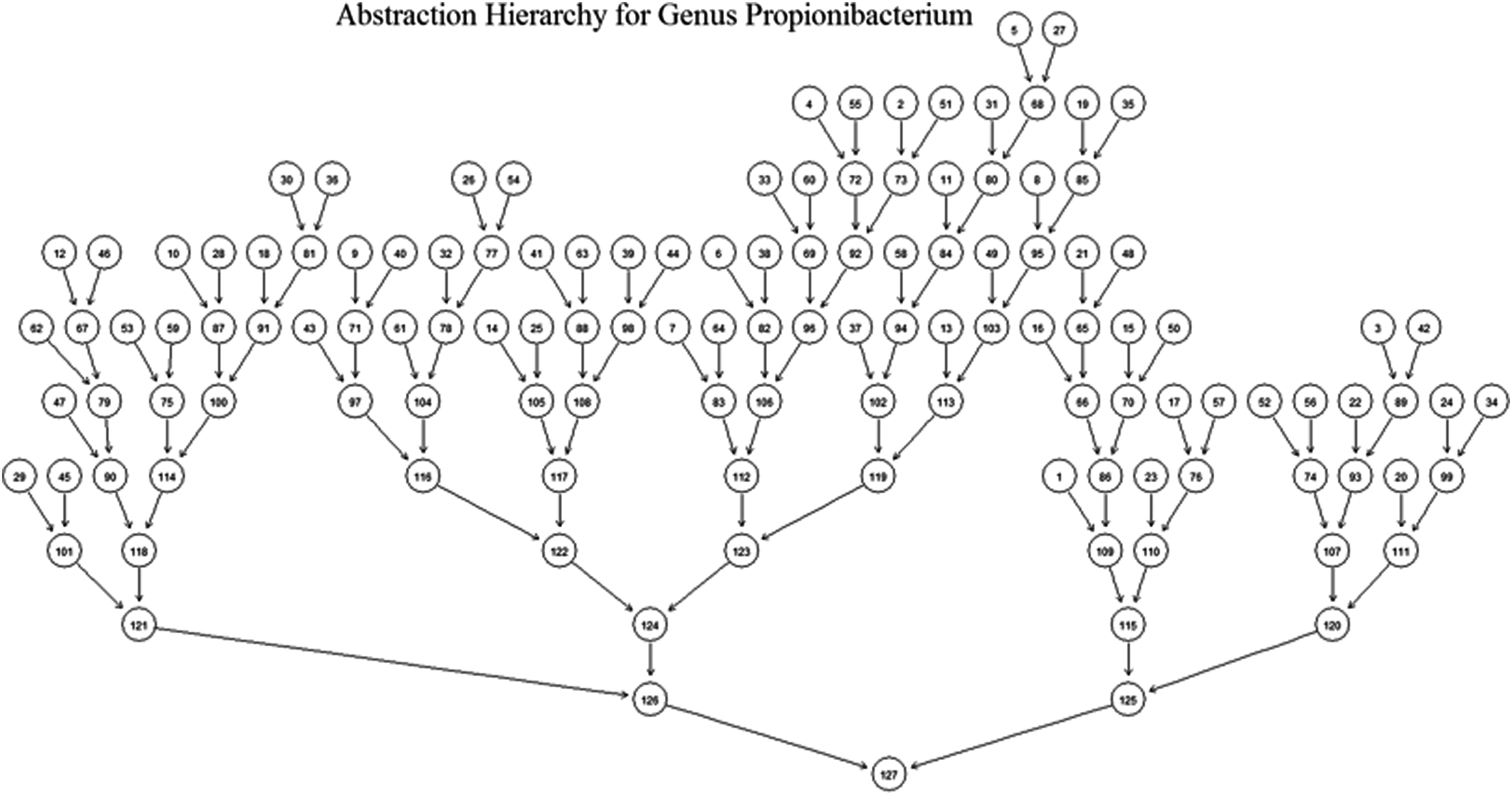
An abstraction hierarchy for the genus Propionibacterium using words of length 3. The leaf nodes at the top represent all 64 possible 3-mers.

In this abstraction hierarchy, the terminal nodes {s₁,…,s₆₄} represent all 64 possible 3-mers. Nodes were recursively merged on the basis of the distance measure given in Equation 2. This abstraction hierarchy describes the similarity of occurrence behavior of 3-mers in genus Propionibacterium; therefore, it could be viewed as a graphical representation of this genus and act as a target model in sequence classification.

2.3. Selecting an M-cut

Recall that an m-cut γ_m through an abstraction hierarchy \documentclass{aastex}\usepackage{amsbsy}\usepackage{amsfonts}\usepackage{amssymb}\usepackage{bm}\usepackage{mathrsfs}\usepackage{pifont}\usepackage{stmaryrd}\usepackage{textcomp}\usepackage{portland, xspace}\usepackage{amsmath, amsxtra}\pagestyle{empty}\DeclareMathSizes{10}{9}{7}{6}\begin{document} $${ \cal T}$$ \end{document} is a subset of m nodes of \documentclass{aastex}\usepackage{amsbsy}\usepackage{amsfonts}\usepackage{amssymb}\usepackage{bm}\usepackage{mathrsfs}\usepackage{pifont}\usepackage{stmaryrd}\usepackage{textcomp}\usepackage{portland, xspace}\usepackage{amsmath, amsxtra}\pagestyle{empty}\DeclareMathSizes{10}{9}{7}{6}\begin{document} $${ \cal T}$$ \end{document} such that for any leaf \documentclass{aastex}\usepackage{amsbsy}\usepackage{amsfonts}\usepackage{amssymb}\usepackage{bm}\usepackage{mathrsfs}\usepackage{pifont}\usepackage{stmaryrd}\usepackage{textcomp}\usepackage{portland, xspace}\usepackage{amsmath, amsxtra}\pagestyle{empty}\DeclareMathSizes{10}{9}{7}{6}\begin{document} $$s_i \in {\cal S}$$ \end{document} , either s_i ∈ γ_m or s_i is a descendant of some node in γ_m. The set of abstractions \documentclass{aastex}\usepackage{amsbsy}\usepackage{amsfonts}\usepackage{amssymb}\usepackage{bm}\usepackage{mathrsfs}\usepackage{pifont}\usepackage{stmaryrd}\usepackage{textcomp}\usepackage{portland, xspace}\usepackage{amsmath, amsxtra}\pagestyle{empty}\DeclareMathSizes{10}{9}{7}{6}\begin{document} $${ \cal A}$$ \end{document} at any given m-cut γ_m forms a partition of \documentclass{aastex}\usepackage{amsbsy}\usepackage{amsfonts}\usepackage{amssymb}\usepackage{bm}\usepackage{mathrsfs}\usepackage{pifont}\usepackage{stmaryrd}\usepackage{textcomp}\usepackage{portland, xspace}\usepackage{amsmath, amsxtra}\pagestyle{empty}\DeclareMathSizes{10}{9}{7}{6}\begin{document} $${ \cal S}$$ \end{document} . To clarify, \documentclass{aastex}\usepackage{amsbsy}\usepackage{amsfonts}\usepackage{amssymb}\usepackage{bm}\usepackage{mathrsfs}\usepackage{pifont}\usepackage{stmaryrd}\usepackage{textcomp}\usepackage{portland, xspace}\usepackage{amsmath, amsxtra}\pagestyle{empty}\DeclareMathSizes{10}{9}{7}{6}\begin{document} $${ \cal S}$$ \end{document} is the leaf set (set containing all p-mers), and each \documentclass{aastex}\usepackage{amsbsy}\usepackage{amsfonts}\usepackage{amssymb}\usepackage{bm}\usepackage{mathrsfs}\usepackage{pifont}\usepackage{stmaryrd}\usepackage{textcomp}\usepackage{portland, xspace}\usepackage{amsmath, amsxtra}\pagestyle{empty}\DeclareMathSizes{10}{9}{7}{6}\begin{document} $$s_i \in { \cal S}$$ \end{document} represents a distinct p-mer. One could also think of s_i as the smallest abstraction of a_i, since an abstraction a_i can contain more than one s_i.

The purpose of scoring an unknown sequence against a target abstraction hierarchy of a known taxon at a preselected level of m-cut is to obtain the posterior probability of unknown query sequence belonging to that known taxon. Abstraction hierarchies are trained by using sequences from the same phylogenetic taxon. Evaluation of each m-cut is based on the posterior probability of the AAMM for a training data set. Given an unknown query sequence {x = x₀, x₁,…,x_(n−1)} and a target abstraction hierarchy with a preselected m-cut gamma_m, the posterior probability for the query sequence is calculated using Equation 5: \documentclass{aastex}\usepackage{amsbsy}\usepackage{amsfonts}\usepackage{amssymb}\usepackage{bm}\usepackage{mathrsfs}\usepackage{pifont}\usepackage{stmaryrd}\usepackage{textcomp}\usepackage{portland, xspace}\usepackage{amsmath, amsxtra}\pagestyle{empty}\DeclareMathSizes{10}{9}{7}{6}\begin{document} \begin{align*}p ( { \bf x} \mid \hat { \theta} ) = p ( x_0 \ldots x_{k - 1} ) \prod_{i = k}^{n - k} \hat{ \theta} ( x_i \mid a^{ \prime}_i ) \tag{5}\end{align*} \end{document}

where p(x₀…,x_k₋₁) is the prior probability of p-mer \documentclass{aastex}\usepackage{amsbsy}\usepackage{amsfonts}\usepackage{amssymb}\usepackage{bm}\usepackage{mathrsfs}\usepackage{pifont}\usepackage{stmaryrd}\usepackage{textcomp}\usepackage{portland, xspace}\usepackage{amsmath, amsxtra}\pagestyle{empty}\DeclareMathSizes{10}{9}{7}{6}\begin{document} $$x_0 \ldots x_{k - 1} , a_i^{ \prime} \in \gamma_m$$ \end{document} is the abstraction that contains p-mer x_i_−k … x_i−1, and \documentclass{aastex}\usepackage{amsbsy}\usepackage{amsfonts}\usepackage{amssymb}\usepackage{bm}\usepackage{mathrsfs}\usepackage{pifont}\usepackage{stmaryrd}\usepackage{textcomp}\usepackage{portland, xspace}\usepackage{amsmath, amsxtra}\pagestyle{empty}\DeclareMathSizes{10}{9}{7}{6}\begin{document} $$\theta^{ \prime} ( x_i \mid a_j^{ \prime} )$$ \end{document} is the posterior probability of observing x_i right after abstraction \documentclass{aastex}\usepackage{amsbsy}\usepackage{amsfonts}\usepackage{amssymb}\usepackage{bm}\usepackage{mathrsfs}\usepackage{pifont}\usepackage{stmaryrd}\usepackage{textcomp}\usepackage{portland, xspace}\usepackage{amsmath, amsxtra}\pagestyle{empty}\DeclareMathSizes{10}{9}{7}{6}\begin{document} $$a_j^{ \prime} /$$ \end{document}

The process of m-cut selection is given by the following algorithm:

1. Specify all possible values of m, {m₀,m₁,…}.

2. Score all training sequences against the abstraction hierarchy for each m_i.

3. Calculate the average of the posterior probabilities for each abstraction (using Equation 5).

4. Return the maximum average posterior probability and the corresponding m-cut.

The main purpose of m-cut selection is to search for the appropriate level of abstractions that best describes the training data set. The performance for sequence classification varies at different levels of target abstractions. Implementing a more specific level (larger m value) of abstractions does not necessarily improve the accuracy of classification, because the parameters may not be accurately estimated if the amount of data at that level is insufficient. On the other hand, classifying sequences at a more general level (smaller m value) of abstractions would not guarantee an improvement in classification performance because there may not be enough terms on the cut to differentiate each class. A simple classification experiment is performed here to illustrate how the m-cut selection affects the classification accuracy.

In all the experiments to evaluate the validity and accuracy of metagenomic classification using AAMM theory, all model training and test sequences are from 16S rRNA sequences, the most widely used genetic marker for bacterial genomes (Case et al., 2007). The sequences are available from the Greenegenes project website (DeSantis et al., 2008). For all experiments, we mainly use 2-mer abstraction hierarchies as the target models in sequence classification, because 16S rRNA sequences, whose average length is around 1500, are comparatively short genetic sequences. Therefore, the parameters in the AAMMs may not be accurately estimated for p-mer abstraction hierarchies if p is greater than two.

In this experiment, the test sequences are from the genera Bacillus, Streptococcus, Clostridium, and Escherichia, since these genera each contain a large number of sequences. We randomly select 20% of the sequences from the Greengenes database in these four genera as the training data set. The test sequences are classified against the corresponding target abstraction hierarchies at all possible levels of abstraction. Figure 4 shows the classification accuracy at all abstraction levels from 2-cut to 16-cut.

FIG. 4.

Classification accuracy rate for m-cuts (abstraction levels) from two to sixteen for four genera from the Greengenes database. The x-axis represents the m-cut level from 2-cut to 16-cut, and the y-axis denotes the classification accuracy rate. Each colored dotted line represents the classification rate for a specific genus. The solid black line is the average classification rate.

From Figure 4, the classification rate varies when the classification is performed at different levels of abstraction (i.e., m-cuts). When classifying test sequences at abstraction level of five-cut, the average classification accuracy is only 60%; however, this changes to nearly 100% when moving to a more specific level of abstraction. It is also clear that each genera has a slightly different pattern of response. For example, the classification rate for the genus Escherichia varies dramatically depending on the abstraction level, while the genus Streptococcus displays a more stable classification rate at various values of m. The main reason is due to the amount of variability within each genus. Genera (and, in general, taxa) with larger intra-variability tend to have unstable classification rates at different m-cut levels. Thus, different genera may have different optimal abstraction levels, and it is important to select an appropriate m-cut for each taxon before performing sequence classification. For these particular genera, the classification rate stabilizes for m ≥ 8.

3. Results

Sequence classification experiments were carried out to evaluate the validity and accuracy of metagenomic classification using AAMMs. For the experiments here, both the Greengenes data set and Yellowstone National Park data sets (described in section 3.1) were imported and processed to use in model learning, m-cut selection, and sequence classification. The Greengenes database was used as training for the Yellowstone data, in order to avoid the bias of classification results due to the sequence replication within one data source. The software was implemented in R (R Core Team, 2014), and the code is available at https://github.com/MonnieMcGee/ZhuMcGeeJCB2015.

3.1. Data sets used

The Greengenes database is a 16S rRNA gene database that addresses limitations of public repositories by providing chimera screening, standard alignment, and taxonomic classification using multiple published taxonomies (DeSantis et al., 2008). The unaligned version of the 16S rRNA sequences from the Greengenes databases are used to train AAHMs to represent each taxon. The total number of sequences we use in this dataset is 406,997, which belong to 94 phyla.

The Department of Energy Joint Genome Institute (DOE-JGI) produced a bacteria-specific 16S rRNA gene library from Yellowstone National Park samples. Samples are from 20 geothermal sites with 35 to 50 megabases of sequence data per site in Yellowstone National Park. Standard Sanger shotgun sequencing (Staden, 1979) was used to obtain genomic samples. This method assembles randomly broken-up DNA segments into continuous sequences using multiple overlapping segments. We refer to this dataset as YNP, and it contains 6026 16S rRNA sequences in 30 phyla. This data set is used to test the performance of AAMMs in metagenomic classification.

3.2. Classification at the phylum level

In order to demonstrate the performance of AAMM for classification of metagenomic data at the phylum level, we designed two phases of experiments. For the first phase of experiments, sequences from the five most abundant phyla in Yellowstone National Park data set were selected as the test sequences. Ten percent of sequences from the Greengenes database in the same five phyla were randomly selected to learn abstraction hierarchies. For each target phylum, the m-cut is selected as described in section 2.3. Then, the entire test sequences were combined and scored against the five abstraction hierarchies at the preselected level of m-cut and were assigned to the phylum with the highest score. The predicted phylum was compared with the actual phylum of the sequence to obtain the classification rate. The list of experimental designs and results is shown in Table 1. The average classification rate for this experiment is 94.26%. As for m-cut selection, three out of five abstraction hierarchies have 15-cut as their optimal level of abstractions, and the other two selected m-cuts of 13 and 14.

Table 1.

Phylum Level Experiments on Large and Midsize Phyla

Phylum name	Sequences from GG	Sequences from YNP	Classification rate (%)
Proteobacteria	12,152	2,726	91.86
Firmicutes	12,256	1969	86.44
Actinobacteria	7,705	442	97.51
Bacteroidetes	4,343	196	98.47
Euryarchaeota	471	135	97.04
Thermi^*	576	58	97.93
Thermotogae^*	445	45	95.60
Synergistetes^*	421	43	93.02
Chlorobi^*	408	41	87.80
SAR406^*	336	34	95.29
TM7^*	264	27	100

For the first five rows in the table, the test sequences for each phylum were selected from the YNP data. The same five sequences were selected from the Greengenes database to train the AAMM. For phyla marked with ^*, all sequences were from the Greengenes database. Ninety percent of the sequences in each phylum were used to train the AAMM, and 10% were used for testing.

In the second phase of phylum level experiments, which are denoted by * in Table 1, sequences from six medium-sized phyla in the Greengenes database were selected to evaluate the performance of gene classification using AAMMs. Each phylum was split up into a ratio of 90% and 10% for training 2-mer abstraction hierarchies and test sequences, respectively. For both large and midsize phyla, all classification rates are above 86%.

3.3. Classification at the genus level

Since it has already been shown that quasi-alignment is more effective than naive Bayes or HMMs for classification at the genus level (Nagar, 2013), we compare the percent of sequences correctly classified from several genera for both AAMM and quasi-alignment. The results are shown in Table 2. For the first phase of this experiment, sequences from the ten most abundant genera in the YNP data set were selected as the test sequences. The training sequences were from the Greengenes data set. We randomly selected 20% of the sequences from the Greengenes database in the same genera to learn abstraction hierarchies and select an optimal m-cut. All test sequences were combined and scored against the ten abstraction hierarchies at preselected abstraction levels and were assigned to the genus with the highest score. The predicted genus was compared with the actual genus of the sequence to obtain the classification rate. The average classification rate for this experiment is 98.62%, and all classification rates are greater than 93%. All ten abstraction hierarchies have 15-cut as their optimal level of abstraction. In each case, the AAMM performs as good as or better than quasi-alignment.

Table 2.

Genus Level Experiments on Large and Midsize Phyla

Genus name	Sequences from GG	Sequences from YNP	AAMM rate (%)	QA rate (%)
Bacillus	1704	434	100	97.2
Streptococcus	1202	275	99.27	99.6
Clostridium	1840	264	100	91.7
Escherichia	214	232	100	98.7
Shewanella	200	228	100	91.7
Lactobacillus	1156	191	93.19	84.4
Burkholderia	354	137	97.08	96.4
Staphylococcus	4600	128	100	97.7
Salmonella	148	121	98.35	89.3
Pseudomonas	2566	118	98.30	99.2

Test sequences for each genus were selected from the YNP data. The same five sequences were selected from the Greengenes database to train the AAMM. The same training and test sets were used for quasi-alignment. In most instances, the AAMM outperforms quasi-alignment in terms of percent correctly classified.

Similarly to the phyla experiments, sequences from 20 medium-sized genera, which contained 154 to 175 sequences, in the Greengenes database were selected to evaluate the performance of gene classification using AAMM's. Each genus was split up into a ratio of 90% and 10% for training and test sequences, respectively. For this experiment, most of the classification rates are 100%; therefore, the results are not shown in detail. For a detailed table of results, see chapter 3 of Zhu (2014).

4. Conclusion

In this article, we reviewed the theory behind AAMM and applied AAMM in metagenomic classification. Detailed algorithms of metagenomic classification we proposed were illustrated, which include model learning, m-cut selection, and sequence classification. Experiments were conducted using 16S rRNA sequences of known microbes. The sequences from the Greengenes data set and Yellowstone National Park data set were divided into training and test sequences at each taxon level. The test sequences were scored against all target abstraction hierarchies at a preselected level in order to determine the predicted taxon. This method has been able to provide accurate classification results at both high and low taxon level, and the average classification rate is above 95%.

The analyses can easily be extended to any set of DNA and RNA sequences. We further compared the sequence classification performance of quasi-alignment method and AAMM method. The two techniques perform similarly; however, the AAMM slightly outperformed quasi-alignment in most cases. These two techniques have the potential to be used in identifying novel species in environmental or biological samples.

With regard to assessing the statistical significance of quasi-alignment and AAMM methods, in future work, we will develop hypothesis tests for the null hypothesis that the query sequence does not belong to a specific taxon in order to provide further information in the classification accuracy. In particular, we will focus on deriving theoretical background distributions for both EMM's supported transition score and AAMM's posterior probability score in order to obtain an accurate representation of the null distribution, and thus an accurate p-value for a hypothesis test. Especially, in regard to EMM construction, further research will concentrate on analytically deriving the distribution of the NSV to the setting where sequence preprocessing step is a renewal process of a Markov Chain. Further research is also required to see how the power of the test behaves in order to better evaluate it. For the extension of application for current quasi-alignment and AAMM methods in sequence classification, further research will aim to apply them in other types of genetic sequences, such as amino acid sequences.

6. Appendix

The following example shows a detailed procedure for calculating the context of the three-cut of the abstraction hierarchy from Figure 1. The procedure for calculating the context of other cuts is similar. In a real sequence classification problem, the value of m is determined by the posterior probability of model training sequences, given in Equation 5. Here, we selected the three-cut as an example for convenience and concreteness.

For the abstraction hierarchy in Figure 1, \documentclass{aastex}\usepackage{amsbsy}\usepackage{amsfonts}\usepackage{amssymb}\usepackage{bm}\usepackage{mathrsfs}\usepackage{pifont}\usepackage{stmaryrd}\usepackage{textcomp}\usepackage{portland, xspace}\usepackage{amsmath, amsxtra}\pagestyle{empty}\DeclareMathSizes{10}{9}{7}{6}\begin{document} $${ \cal D}$$ \end{document} = {abracadabra}, χ = {a, b, c, d, r}, and \documentclass{aastex}\usepackage{amsbsy}\usepackage{amsfonts}\usepackage{amssymb}\usepackage{bm}\usepackage{mathrsfs}\usepackage{pifont}\usepackage{stmaryrd}\usepackage{textcomp}\usepackage{portland, xspace}\usepackage{amsmath, amsxtra}\pagestyle{empty}\DeclareMathSizes{10}{9}{7}{6}\begin{document} $${ \cal S}$$ \end{document} = {ra, ca, da, ab,br, ac, ad}. The three-cut for this hierarchy is a unique partition of \documentclass{aastex}\usepackage{amsbsy}\usepackage{amsfonts}\usepackage{amssymb}\usepackage{bm}\usepackage{mathrsfs}\usepackage{pifont}\usepackage{stmaryrd}\usepackage{textcomp}\usepackage{portland, xspace}\usepackage{amsmath, amsxtra}\pagestyle{empty}\DeclareMathSizes{10}{9}{7}{6}\begin{document} $${ \cal S} ,$$ \end{document} which contains nodes {a₁₀.a_s,a₈}. In order to find the three-cut, we first calculate the contact of all existing 2-mers. For example, the context of s₁ = {ra} for character a, based on the Smith–Waterman algorithm for local alignment (Smith and Waterman, 1981), is \documentclass{aastex}\usepackage{amsbsy}\usepackage{amsfonts}\usepackage{amssymb}\usepackage{bm}\usepackage{mathrsfs}\usepackage{pifont}\usepackage{stmaryrd}\usepackage{textcomp}\usepackage{portland, xspace}\usepackage{amsmath, amsxtra}\pagestyle{empty}\DeclareMathSizes{10}{9}{7}{6}\begin{document} \begin{align*}\hat { \theta } _ { \displaystyle a \mid s_1 } = \hat { \theta } _ { \displaystyle a \mid ra } = { \frac { 1 + f [ s_1a ] } { 5 + f [ s_1a ] + f [ s_1b ] + f [ s_1c ] + f [ s_1d ] + f [ s_1r ] } } = { \frac { 1 + 0 } { 5 + 1 } } = \frac { 1 } { 6 } , \tag { 6 } \end{align*} \end{document}

which means that the conditional probability of observing character a right after 2-mer s₁ = {ra} is one-sixth. We can calculate the context of all two-mers in a similar manner. The results are given in Table 3.

Table 3.

The Calculated Context for All 2-mers

\documentclass{aastex}\usepackage{amsbsy}\usepackage{amsfonts}\usepackage{amssymb}\usepackage{bm}\usepackage{mathrsfs}\usepackage{pifont}\usepackage{stmaryrd}\usepackage{textcomp}\usepackage{portland, xspace}\usepackage{amsmath, amsxtra}\pagestyle{empty}\DeclareMathSizes{10}{9}{7}{6}\begin{document} $$ \hat { \theta}_{ \sigma \mid s}$$ \end{document} ₁	s₁ = ra	s₂ = ca	s₃ = da	s₄ = ab	s₅ = br	s₆ = ac	s₇ = ad
a	1/6	1/6	1/6	1/7	3/7	2/6	2/6
b	1/6	1/6	2/6	1/7	1/7	1/6	1/6
c	2/6	1/6	1/6	1/7	1/7	1/6	1/6
d	1/6	2/6	1/6	1/7	1/7	1/6	1/6
r	1/6	1/6	1/6	3/7	1/7	1/6	1/6

For example, the conditional probability of observing character a right after two-mer s₄ = {br} is 3/7, and the conditional probability of observing character c right after two-mer s₃ = {da} is 1/6.

Now that we have the context of the 2-mers, we can calculate the context of the abstractions. Since a₁₀ = {ra, ca, da} = {s₁, s₂, s₃}, on the basis of the Poisson distribution (Karlin and Altschul, 1990), the context of abstraction a₁₀ for character a is. \documentclass{aastex}\usepackage{amsbsy}\usepackage{amsfonts}\usepackage{amssymb}\usepackage{bm}\usepackage{mathrsfs}\usepackage{pifont}\usepackage{stmaryrd}\usepackage{textcomp}\usepackage{portland, xspace}\usepackage{amsmath, amsxtra}\pagestyle{empty}\DeclareMathSizes{10}{9}{7}{6}\begin{document} \begin{align*}\hat { \theta } _ { \displaystyle a \mid a_ { 10 } } = { \frac { 1 + f [ s_1 ] } { 3 + f [ s_1 ] + f [ s_2 ] + f [ s_3 ] } } \hat \theta _ { \displaystyle a \mid s_1 } + { \frac { 1 + f [ s_2 ] } { 3 + f [ s_1 ] + f [ s_2 ] + f [ s_3 ] } } \hat \theta _ { \displaystyle a \mid s_2 } + { \frac { 1 + f [ s_3 ] } { 3 + f [ s_1 ] + f [ s_2 ] + f [ s_3 ] } } \hat \theta _ { \displaystyle a \mid s_3 } = \frac { 1 } { 6 } , \tag { 7 } \end{align*} \end{document}

which means that the conditional probability of observing character a right after a set of 2-mers a₁₀ = {ra, ca, da} = 1/6. Similarly, Table 4 lists the context of abstractions {a₁₀, a₃, a₈}. Once the distance between two abstractions is defined, we can train abstraction hierarchies using known sequences.

Table 4.

The Context of Abstractions {a₁₀, a₃, a₈}

\documentclass{aastex}\usepackage{amsbsy}\usepackage{amsfonts}\usepackage{amssymb}\usepackage{bm}\usepackage{mathrsfs}\usepackage{pifont}\usepackage{stmaryrd}\usepackage{textcomp}\usepackage{portland, xspace}\usepackage{amsmath, amsxtra}\pagestyle{empty}\DeclareMathSizes{10}{9}{7}{6}\begin{document} $$ \hat { \theta}_{ \sigma \mid { \rm s}_{ \rm i}}$$ \end{document}	a₁₀ = {s₁,s₂,s₃}	a₃ = s₄	a₈ = {s₅,s₆,s₇}
a	1/6	1/7	55/147
b	3/14	1/7	23/147
c	5/21	1/7	23/147
d	3/14	1/7	23/147
r	1/6	3/7	23/147

For example, the conditional probability of observing character b immediately after a set of two-mers a₁₀ = {ra,ca,da} is 3/14, and the conditional probability of observing character d immediately after a set of two-mers a₈ = {br, ac, ad} is also 3/14.

Footnotes

Acknowledgments

This work was funded by the National Institutes of Health Developmental Research Grant Program (Parent R21) to Michael Hahsler (PI) and Monnie McGee (Co-PI), grant number 1 R21 HG005912-01A1.

Author Disclosure Statement

No competing financial interests exist.

References

Almeida

J.S.

, and Vinga

2002. Universal sequence map (USM) of aribitrary discrete sequences. BMC Bioinform., 3, 6.

Altschul

S.F.

, Gish

, Miller

, et al. 1990. Basic local alignment search tool. J. Mol. Biol., 215, 403–410.

Blaisdell

B.E.

1986. A measure of similarity of sets of sequences not requiring sequence alignment. Proc. Natl. Acad. Sci. U.S.A., 83, 5155–5159.

Blaisdell

B.E.

1989. Effectiveness of measures requiring and not requiring prior sequence alignment for estimating the dissimilarity of natural sequences. J. Mol. Evol., 29, 526–537.

Caragea

2009. Abstraction-based probabilistic models for sequence classification. Department of Computer Science, Iowa State University.

Caragea

, Silvescu

, Caragea

, and Honavar

2009. Abstraction augmented Markov models. NIPS Workshop on Machine Learning in Computational Biology. Vancouver, BC, Canada.

Case

R.J.

, Boucher

, Dahllof

, et al. 2007. Use of 16s rrna and rpob genes as molecular markers for microbial ecology studies. Appl. Environ. Microbiol., 73, 278–288.

Charfreitag

, and Stackebrandt

1989. Inter- and intragenic relationships of the genus propionbacterium as determined by 16s rrna sequences. Microbiology, 135, 2065–2070.

Clemente

J.C.

, Jansson

, and Valiente

2011. Flexible taxonomic assignment of ambiguous sequencing reads. BMC Bioinform., 12, 8.

10.

Consortium

I.H.G.S.

2001. Initial sequencing and analysis of the human genome. Nature, 409, 860–921.

11.

DeSantis

, Hugenholtz

, Larsen

, et al. 2008. Greengenes, a chimera-checked 16s rRNA gene database and workbench compatible with ARB. Appl. Environ. Microbiol., 72, 5069–5072.

12.

Dunham

M.H.

, Meng

, and Huang

2004. Extensible Markov model, 371–374. In Proceedings of the Fourth IEEE International Conference on Data Mining. IEEE, New York.

13.

Enright

A.J.

, Iliopoulos

, Kyrpides

N.C.

, and Ouzounis

C.A.

1999. Protein interaction maps for complete genomes based on gene fusion events. Nature, 402, 86–90.

14.

Fichant

, and Gautier

1987. Statistical method for predicting protein coding regions in nucleic acid sequences. Comput. Appl. Biosci., 3, 287–295.

15.

Fuhrman

J.A.

2012. Metagenomics and its connection to microbial community organization. F1000 Biol. Rep., 4, 15.

16.

Gibbs

A.J.

, Dale

, Kinns

, and MacKenzie

1971. The transition matrix method for comparing sequences: Its use in describing and classifying proteins by their amino acid sequences. Syst. Zool., 20, 417–425.

17.

Hahsler

, and Nagar

2014. Quasialign: Infrastructure for quasi-alignment of genetic sequences. R Package Version 0.0-4.

18.

Hide

, Burke

, and Davison

D.B.

1994. Biological evaluation of d2, an algorithm for high-performance sequence comparison. J. Comput. Biol., 1, 199–215.

19.

Hugenholtz

, Goebel

B.M.

, and Pace

N.R.

1998. Impact of culture-independent studies on the emerging phylogenetic view of bacterial diversity. J. Bacteriol., 180, 6793.

20.

Huson

D.L.

, Auch

A.F.

, Qi

, and Schuster

S.C.

2007. Megan analysis of metagenomic data. Genome Res., 17, 377–386.

21.

Karlin

, and Altschul

1990. Methods for assessing the statistical significance of molecular sequence features by using general scoring schemes. Proc. Natl. Acad. Sci. U.S.A., 87, 2264–2268.

22.

Kim

, Lee

K.-H.

, Yoon

S.-W.

, et al. 2013. Analytical tools and databases for metagenomics in the next-generation sequencing era. Genomics Informat., 11, 102–113.

23.

Kotamarti

R.M.

, Hahsler

, Raiford

, et al. 2010. Analyzing classification using extensible Markov models. Bioinformatics, 26, 2235–2241.

24.

, Badger

J.H.

, Chen

, et al. 2001. An information-based sequence distance and its application to whole mitochondrial genome phylogeny. Bioinformatics, 17, 149–154.

25.

Lin

1991. Divergence measures based on the shannon entropy. IEEE Trans. Inf. Theory, 37, 145–151.

26.

Nagar

2013. A quasi-alignment based framework for fast discovery of conserved regions and classification of DNA fragments [Ph.D. dissertation]. Southern Methodist University.

27.

R Core Team. 2014. R: A Language and Environment for Statistical Computing. R Foundation for Statistical Computing, Vienna, Austria.

28.

Smith

T.F.

, and Waterman

M.S.

1981. Identification of common molecular subsequences. J. Mol. Biol., 147, 195–197.

29.

Solovyev

V.V.

, and Makarova

K.S.

1993. A novel method of protein sequence classification based on oligopeptide frequency analysis and its application to search for functional sites and to domain localization. Bioinformatics, 9, 17–24.

30.

Staden

1979. A strategy of DNA sequencing employing computer programs. Nucleic Acids Res., 6, 2601–2610.

31.

Stuart

G.W.

, Moffett

, and Baker

2002. Integrated gene and species phylogenies from unaligned whole genome protein sequences. Bioinformatics, 18, 100–108.

32.

Torney

D.C.

, Burks

, Davison

D.B.

, and Sirotkin

K.M.

1990. A simple measure of sequence divergence. Technical Report LAUR 89-946, Los Alamos National Laboratory.

33.

Turnbaugh

P.J.

, Ley

R.E.

, Harnady

, et al. 2007. The Human Microbiome Project: Exploring the microbial part of ourselves in a changing world. Nature, 449, 804–810.

34.

van Heel

1991. A new family of powerful multivariate statistical sequence analysis techniques. J. Mol. Biol., 220, 877–887.

35.

Wang

, Garrity

G.M.

, Tiedje

J.M.

, and Cole

J.R.

2007. Naive Bayesian classifier for rapid assignment of rRNA sequences into the new bacterial taxonomy. Appl. Environ. Microbiol., 73, 5261–5267.

36.

Weisburg

W.G.

, Barns

S.M.

, Pelletier

D.A.

, and Lane

D.J.

1991. 16s ribosomal DNA amplification for phylogenetic study. J. Bacteriol., 173, 697–703.

37.

T.-J.

, Burke

, and Davison

D.B.

1997. A measure of DNA sequence dissimilarity based on Mahalanobis distance between frequencies of words. Biometrics, 53, 1431–1439.

38.

T.-J.

, Hsieh

Y.-C.

, and Li

L.-A.

2001. Statistical measures of DNA sequence dissimilarity under Markov chain models of base composition. Biometrics, 57, 441–448.

39.

Yoon

B.-J.

2009. Hidden Markov models and their applications in biological sequence analysis. Curr. Genomics, 10, 402–415.

40.

Zhu

X.S.

2014. Comparison of quasi-alignment methods for metagenomic classification. Department of Statistical Science, Southern Methodist University.

\documentclass{aastex}\usepackage{amsbsy}\usepackage{amsfonts}\usepackage{amssymb}\usepackage{bm}\usepackage{mathrsfs}\usepackage{pifont}\usepackage{stmaryrd}\usepackage{textcomp}\usepackage{portland, xspace}\usepackage{amsmath, amsxtra}\pagestyle{empty}\DeclareMathSizes{10}{9}{7}{6}\begin{document} $$ \hat { \theta}_{ \sigma \mid s}$$ \end{document} ₁	s₁ = ra	s₂ = ca	s₃ = da	s₄ = ab	s₅ = br	s₆ = ac	s₇ = ad
a	1/6	1/6	1/6	1/7	3/7	2/6	2/6
b	1/6	1/6	2/6	1/7	1/7	1/6	1/6
c	2/6	1/6	1/6	1/7	1/7	1/6	1/6
d	1/6	2/6	1/6	1/7	1/7	1/6	1/6
r	1/6	1/6	1/6	3/7	1/7	1/6	1/6

\documentclass{aastex}\usepackage{amsbsy}\usepackage{amsfonts}\usepackage{amssymb}\usepackage{bm}\usepackage{mathrsfs}\usepackage{pifont}\usepackage{stmaryrd}\usepackage{textcomp}\usepackage{portland, xspace}\usepackage{amsmath, amsxtra}\pagestyle{empty}\DeclareMathSizes{10}{9}{7}{6}\begin{document} $$ \hat { \theta}_{ \sigma \mid s}$$ \end{document} ₁	s₁ = ra	s₂ = ca	s₃ = da	s₄ = ab	s₅ = br	s₆ = ac	s₇ = ad
a	1/6	1/6	1/6	1/7	3/7	2/6	2/6
b	1/6	1/6	2/6	1/7	1/7	1/6	1/6
c	2/6	1/6	1/6	1/7	1/7	1/6	1/6
d	1/6	2/6	1/6	1/7	1/7	1/6	1/6
r	1/6	1/6	1/6	3/7	1/7	1/6	1/6

\documentclass{aastex}\usepackage{amsbsy}\usepackage{amsfonts}\usepackage{amssymb}\usepackage{bm}\usepackage{mathrsfs}\usepackage{pifont}\usepackage{stmaryrd}\usepackage{textcomp}\usepackage{portland, xspace}\usepackage{amsmath, amsxtra}\pagestyle{empty}\DeclareMathSizes{10}{9}{7}{6}\begin{document} $$ \hat { \theta}_{ \sigma \mid s}$$ \end{document} ₁	s₁ = ra	s₂ = ca	s₃ = da	s₄ = ab	s₅ = br	s₆ = ac	s₇ = ad
a	1/6	1/6	1/6	1/7	3/7	2/6	2/6
b	1/6	1/6	2/6	1/7	1/7	1/6	1/6
c	2/6	1/6	1/6	1/7	1/7	1/6	1/6
d	1/6	2/6	1/6	1/7	1/7	1/6	1/6
r	1/6	1/6	1/6	3/7	1/7	1/6	1/6