
Abstract
Abstract
1. Introduction
L
There have been several methods developed for differential abundance analysis with RNA-seq data and gene expression analysis. Those analytical tools including edgeR and DESeq (Robinson et al., 2010; Anders and Huber, 2010; Li et al., 2012; Young et al., 2012; Mortazavi et al., 2008) may be applicable to metagenomic data analysis, because both data are from sequencing-based technologies. However, metagenomics data have specific characteristics that need to be considered. Compared to RNA-seq data, metagenomic data are more sparse, with many zeros. In addition, metagenomics data need to be preprocessed into proportion (compositions) for adjusting biases in read-depth across different samples. Therefore, specific tools for dealing with such compositional data have to be developed. Recently, the problem of assessing differential expression in sparse high-throughput microbial marker-gene survey data has been addressed by introducing a cumulative-sum scaling (CSS) and zero-inflated Gaussian (ZIG) model (Paulson et al., 2013). R package “metagenomeSeq” was developed for the implementation of the proposed approach. It was shown that metagenomeSeq outperforms other tools currently used in this field. However, metagenomeSeq did not handle the compositional data directly. The data was first normalized with cumulative sum scaling, and then ZIG model was applied. The normalized data is sometimes hard to explain.
To overcome the limitations of existing methods for metagenomics analysis, we propose a zero-inflated beta regression approach to handle the proportion data directly. Beta regression is an extension of the generalized linear model (GLM) approach with the assumption that proportional dependent variable can be characterized by the beta distribution. Beta distribution is well known to be flexible for modeling proportional data (Johnson et al., 1993; Ospina et al., 2012). Zero-inflated beta regression incorporates the existing beta distribution with a degenerate distribution, allowing for modeling metagenomics compositional data efficiently (Stasinopoulos and Rigby, 2007). Under various simulations, we show that ZIBSeq performs well for all these types of distributions, especially that it significantly outperforms other methods for features with sparse counts. We also demonstrate the utility of our method on real human metegenomics data. Biologically significant taxa are identified with ZIBSeq. ZIBSeq can be directly applied to the comparison of more than two clinical conditions or continuous outcome variables without difficulty.
2. Methods
We seek to construct an efficient method that takes the compositional nature of the data into account, deals with sparsity efficiently, and is flexible enough to perform well in various conditions.
(ii) Transformation. When the distributions of the proportion are extremely left skewed, that is, most of the nonzero proportions are very small, the assumption of beta distribution may not be satisfied. In such cases, some appropriate transformations such as square root transformation
2.1. Differential abundance analysis via zero-inflated beta regression
Since beta distribution has a wide range of different shapes depending on the values of two parameters, beta regression models (Ferrari and Cribari-Neto, 2004) are very useful when the response variables are continuous and restricted to the interval (0,1). Assume that x follows a beta distribution denoted as x∼beta(μ,φ), where μ(0 < μ < 1) is the mean and φ (φ > 0) is a precision parameter. The beta density then can be described as a function of μ and φ (Ferrari and Cribari-Neto, 2004):
where Γ(·) is the gamma function. Under this parameterization,
To deal with the case when interested variable contains zero or one, a more general class of zero-or-one inflated beta regression models for continuous proportions was recently proposed by Ospina and Ferrari (2012). Since zero instead of one is very frequently observed in metagenomics data, in this article, we only consider the zero-inflated beta regression, which assumes the response variable has a mixed continuous-discrete distribution with probability mass at zero. For zero-inflated beta distribution, a new parameter α is added to account for the probability of observations at zero. The subsequent mixture density is:
where f (x; μ,φ) is the beta density (1) and α is the probability of observing zero.
Let
where
On the other hand, if the proportion x follows a beta distribution under parameterization in (1), then we have
From (4) and (5) it is easy to obtain an approximation of the dispersion parameter φ:
We implemented this result in Equation (3).
Aims to control the false discovery rate (FDR), q-value has been widely accepted as an alternative approach for multiple hypothesis testing correction in recent years (Benjamini, 2010). In this article, the significance of a differential test is measured by a q-value calculated using the algorithm developed by Storey and Tibshirani (2003). Under the assumption that p-values are uniformly distributed, this method will yield conservative q-value estimates. Our method can be summarized as below:
3. Results
We first present the results of four simulation studies to evaluate and compare ZIBSeq (zib), ZIBSeq with square root transformed response variable (zib_sqrt), and metagenomeSeq (zig) discussed in section 2. Then, one case study on real data will show how ZIBSeq is employed to find meaningful features in genomic studies.
3.1. Simulation
In order to compare the abilities of zib, zib_sqrt, and zig in detecting differentially expressed features, simulations were designed to generate data from four common types of distributions: zero-inflated Poisson distribution (ZIP), zero-inflated negative binomial distribution (ZINBI), multinomial distribution (MN), and binomial distribution (BI). All methods use standard approaches of false discovery rate (FDR) and q-value (Benjamini and Hochberg, 1995) for multiple hypothesis correction. Differentially abundant features were determined at FDR <0.05. To evaluate the ability of ZIBSeq and metagenomeSeq in identifying differential features, R package ROCR (Sing et. al, 2005) is employed to perform the ROC analysis. In each simulation, ROC curves and area under the curve (AUC) values were averaged by 100 random experiments.
In simulations on zero-inflated Poisson distribution ZIP(α,μ) and zero-inflated negative binomial distribution ZINBI(α,μ,σ) (Johnson et al., 1993), 5 out of 100 features were set to be differentially expressed, with means μ = {5, 5, 50, 300, 500} and {6, 8, 60, 350, 600}, respectively. The remaining 95 genes were generated from the same distribution with μ varied from 5 to 750. The probability of zero α is chosen to be 0.05 in both simulations, while the dispersion parameter is σ = 0.1 in zero-inflated negative binomial distribution.
To get reasonable values in simulations on multinomial distribution MN(
ROC curves were shown in Figures 1 and 2 to illustrate the performance of the two methods in detecting significant features for sample size n = 200 and n = 50, respectively. Corresponding AUC values were calculated and listed in Table 2 to compare the performance of ZIBSeq and metagenomeSeq on data from these four distributions.
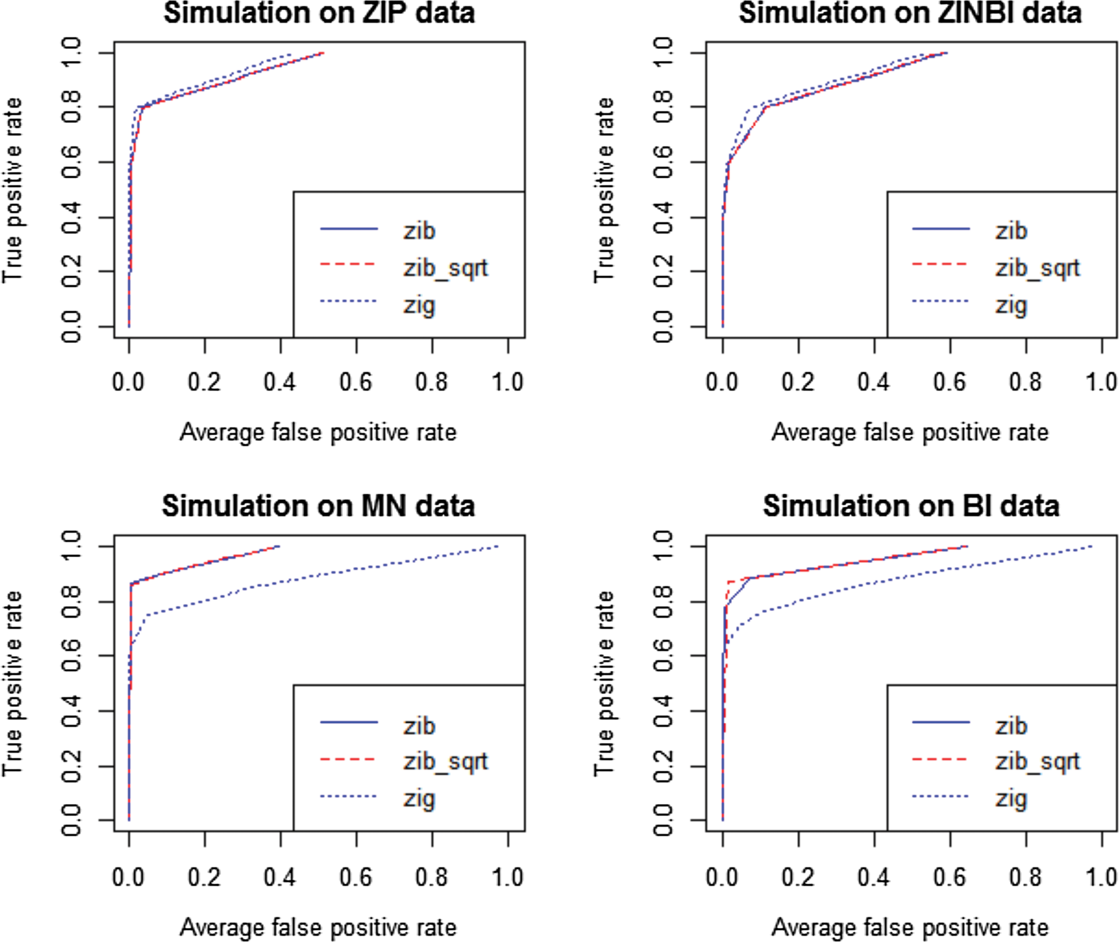
Comparison of ZIBSeq (zib), ZIBSeq with square root transformation (zib_sqrt), and metagenomeSeq (zip) based on simulated data from zero-inflated Poisson distribution (ZIP), zero-inflated negative binomial distribution (ZINBI), multinomial distribution (MN), binomial distribution (BI), and n = 200.
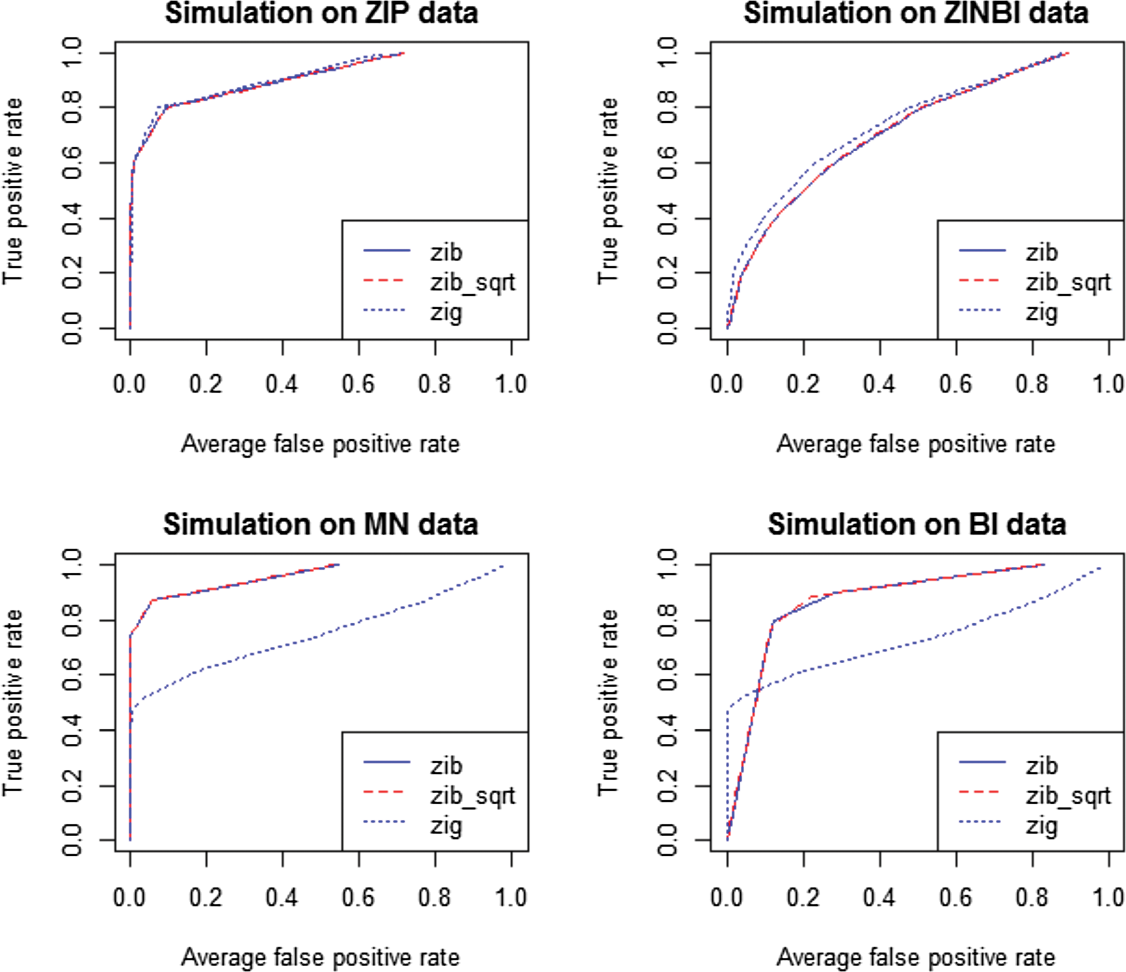
Comparison of ZIBSeq (zib), ZIBSeq with square root transformation (zib_sqrt), and metagenomeSeq (zip) based on simulated data from zero-inflated Poisson distribution (ZIP), zero-inflated negative binomial distribution (ZINBI), multinomial distribution (MN), binomial distribution (BI), and n = 50.
As shown from Figure 1 and 2 and Table 2, all methods (zib, zib_sqrt, and zig) performed similarly on ZIP and ZINBI data. With the sample size 200, the average AUCs of zib and zib_sqrt methods for ZIP data were 0.983, and for ZINBI data were 0.944 and 0.945, respectively, while the average AUCs of zig model for ZIP and ZINBI data were 0.991 and 0.959, respectively. Similar results were achieved with the sample size 50, indicating that zig performed slightly better than zib and zib_sqrt with larger AUC values at different sample sizes. However, it is clear that zib and zib_sqrt were more effective than zig on MN and BI data. With the sample size 200, both zib and zib_sqrt achieved the AUC of 0.999 for MN data and achieved the AUC of 0.998 for MN data respectively, while zig only had the average AUCs of 0.897 and 0.873, respectively. The advantages of zib and zib_sqrt are more significant with a smaller sample size of n = 50. Both zib and zib_sqrt had the average AUCs of 0.980 for ZIP data, and 0.955 for ZINBI data, while zig only achieved the average AUCs of 0.761 and 0.740 for MN and BI data, respectively. In all simulations, zib and zib_sqrt performed almost the same.
3.2. Real metagenomic data
The metagenomic dataset was downloaded from dbGaP under study ID phs000258. The data and analytical results were first reported by Zupancic et al. (2012). There were a total of 310 Amish adult samples with 112 males and 198 females. After aligning the 16S rRNA sequences of gut microbiota to reference sequences and taxonomy databases, there were a total of 240 taxa at the genus level. The clinical phenotype we study is the body mass indices (BMI). The average BMIs are 27.2 and 30.3 for male and female, respectively. We try to identify BMI-associated genera with the proposed approach. We first drop the taxa with average reads below 2, because taxa with a small number of reads are not reliable and subject to noises and measurement errors. There are 62 out of 240 features that average more than 2 reads left for further studies. BMI can be treated as either an ordinal or categorical variable with normal (N: BMI < 25), overweight (OW: 25 ≤ BMI < 30), obese (OB: 30 ≤ BMI ≤ 40), and morbidly obee (OM: BMI > 40). We first treated BMI as a categorical variable and applied zib and zib_sqrt to N + OW + OB vs OM. Two taxa including Faecalibacterium and Ruminococcus were identified with both zib and zib_sqrt with FDR < 0.05. The same two taxa were selected with zib, but three taxa including an additional, Collinsella (besides Faecalibacterium and Ruminococcus), are chosen when considering the BMI group as ordinal variables as shown in Figure 3.
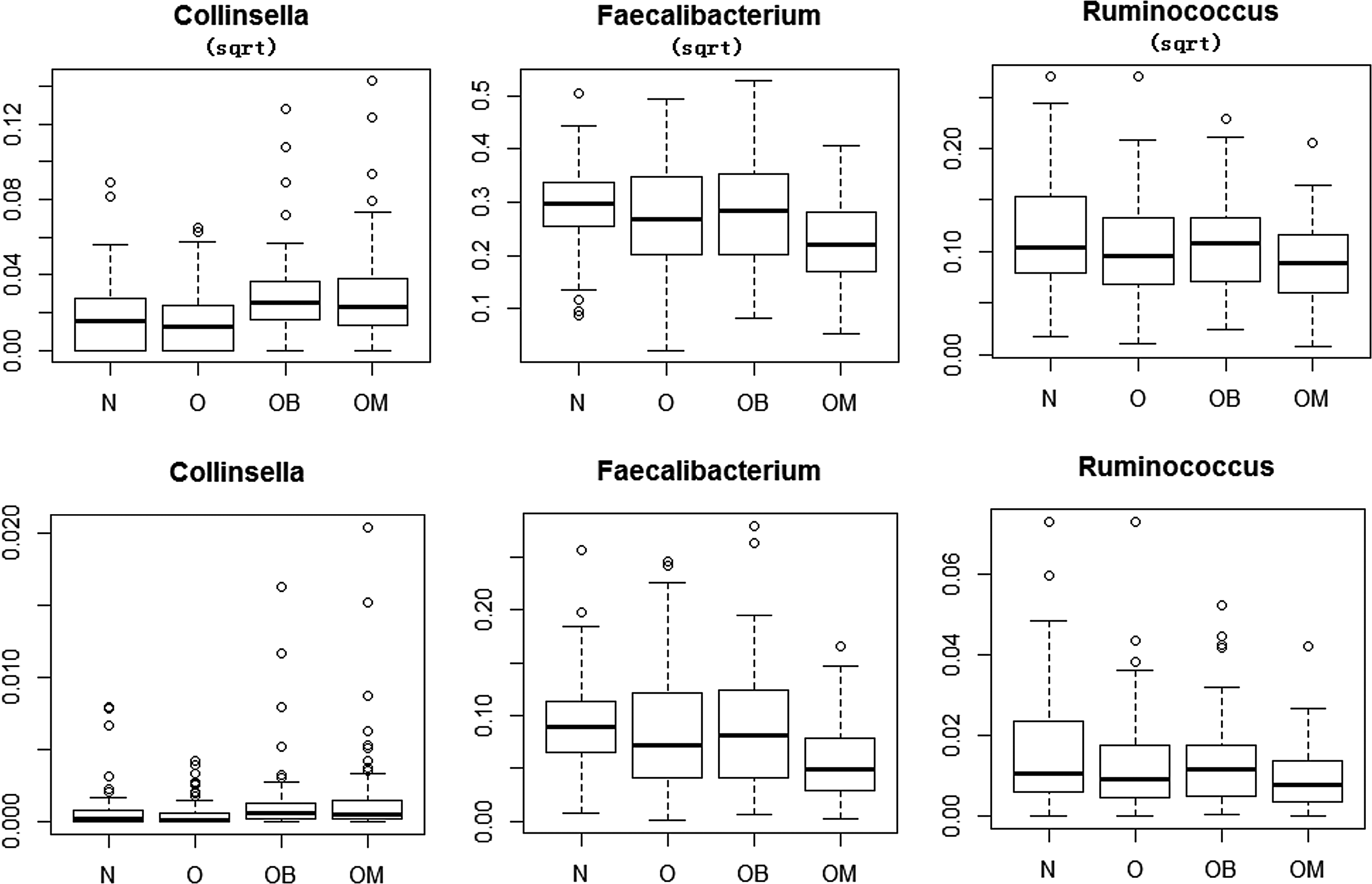
Boxplots of Collinsella, Faecalibacterium, and Ruminococcus as square root transformations (first row) and proportion (second row) for four BMI groups.
Also shown in Figure 3, both Faecalibacterium and Ruminococcus have lower relative abundance in the morbid obesity group, while Collinsella has higher relative abundance in both obese and morbidly obee groups. It is well known that intestinal microbiota composition varies between healthy and diseased individuals for numerous diseases including obesity. It has been shown in the literature that Faecalibacterium was significantly increased in response to dietary factors and weight loss (Remely et al., 2015) and was suggested as a target for intervention (Thomas et al., 2014). Both Ruminococcus and Collinsella are less studied, but there was evidence indicating that the relative abundance of Ruminococcus varies between obese and nonobese individuals (Kasaiet al., 2015). The biological importance of Collinsella needs to be further explored.
4. Discussion
We proposed ZIBSeq tools to handle the metagenomics compositional data with many zeros efficiently. When compared with the popular zig model, our approach performed well with various kinds of data, especially with data simulated from multinomial and binomial distributions. In addition, even though negative q-values were sometimes observed in simulations based on MN and BI data for all methods, zig approach is more likely to obtain negative q-values since it tends to produce more small p-values, which violates the assumption of uniform distribution in the q-value calculation algorithm proposed by Storey and Tibshirani (2003). Benefitting from the flexibility of beta distribution, our method is more stable. It can also identify biologically important taxa in a real application.
Footnotes
Acknowledgments
This work was partially supported by the National Science Foundation (NSF) grant DMS-222381 (Z.L.), NSFC grant 10726054 (X.P.), and NIH grants 5P30CA-16042 and 8UL1TR000124 (G.L.). The funders had no role in the preparation of this article.
Author Disclosure Statement
The authors declare that no competing financial interests exist.