Resolving Conflicting Predictions from Multimapping Reads

Abstract

The first step in the analysis of data produced by ultra-high-throughput next-generation sequencing technology is to map short sequence “reads” to a reference genome, if available. Sequencing errors, repeat regions, and polymorphisms may lead a read to align to multiple locations in the genome reasonably well. While ignoring such multimapping reads, or some of their alignments, will reduce the sensitivity of almost any type of downstream analysis (e.g., detecting structural variants), erroneous mappings will typically yield false positive predictions. Here we propose a framework that aims to identify true predictions among a large set of candidate predictions by selecting for each read a unique mapping that collectively imply conflict-free predictions. We formulate this problem as the maximum facility location problem, for which we propose LP-rounding heuristics. We provide a theoretic guarantee on the quality of the solution and demonstrate the utility of our algorithm in resolving conflicting deletions implied by simulated reads mapping ambiguously to Craig Venter's genome model and Illumina sequencing reads of the well-studied NA12878 individual.

1. Introduction

Ultra-high-throughput next-generation sequencing (NGS) instruments generate a huge number of short DNA sequences, so-called “reads,” that can be mapped back to their origin in a reference genome to facilitate the reconstruction of the desired biological measurement from the individual puzzle pieces. The correct mapping of a read to its true origin, however, is hampered by sequencing errors and genuine differences between reference and donor genomes which enlarge the search space by inexact read matches and thus might lead, similar to repetitive regions, to ambiguous mappings. Furthermore, assay-specific read characteristics like bisulfite-converted DNA (BS-seq) or introns spanned by RNA-seq reads might further complicate the search for the true origin of a read.

Simply ignoring ambiguously mapping reads in the reconstruction of, for example, genomic polymorphisms, alternative splicing, or DNA methylation, has a negative impact on the sensitivity of the prediction, especially in repeat regions of the genome. In Hach et al. (2010), for example, 100 bp reads mapped on average to 140 locations with at most six mismatches in the human reference genome. Not surprisingly, neglecting all but one arbitrary mapping in the downstream analysis will yield both false positive and false negative predictions.

A common approach to unify the (ambiguous) mappings of different reads is to derive an overall set of candidate predictions from all maximal groups of read mappings that support the same phenomenon. To improve sensitivity within repetitive regions of the genome, current methods for structural variant detection form clusters (or cliques) based on all good read alignments (Medvedev et al., 2009), not just one best alignment. Since segmental duplications define hotspots for large-scale variations (Cooper et al., 2007; Kim et al., 2008), these regions are of particular interest (Medvedev et al., 2009). The main challenge this soft clustering strategy has to cope with is that of maintaining a high precision. The candidate set it generates naturally contains a significant number of false positive predictions, since ambiguous mappings of a single read may participate in several predictions although at most one of them denotes the true origin.

In this work, we propose a model and algorithms to separate true predictions from candidate predictions that result from mapping artefacts. To be applicable to a wide range of interpretation problems of NGS read mappings, we solely employ the conflict of different predictions to resolve ambiguous mappings. We refrain from imposing additional assumptions like parsimony. We formulate the unique assignment of multimapping reads to conflict-free predictions as a global optimization problem that takes into account the entirety of all (ambiguous) read mappings. The algorithm we propose resolves conflicts among predictions efficiently based on the assumption that predictions can be represented by genomic intervals with respect to the reference, and that two predictions are in conflict if and only if the corresponding intervals overlap. For example, introns inferred from spliced alignments of RNA-seq reads, deletions in a donor genome with respect to a reference genome (see overlapping green and red deletion in Fig. 1), and other types of genetic variations like inversions naturally correspond to nonoverlapping genomic intervals. This does not only apply to haploid genomes, but also in diploid genomes, for example, overlapping (but different) deletions or introns represent rare events.

FIG. 1.

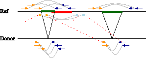
Alignments supporting conflicting deletions. An orange and a blue read connected by a gray line represent a paired-end read. The two reads map to the reference genome at a distance larger than the distance between the sequenced ends (reads) of the donor fragments, indicating a potential deletion. Alternative (wrong) alignments (red dotted lines) support a (wrong) deletion (red) that overlaps the green deletion to the left and thus the two deletions cannot occur simultaneously on the same allele.

1.1. Preliminaries

We formulate the problem of resolving conflicting predictions from multimapping reads as the maximum facility location problem, which we formally introduce in the next section. A set of clients has to be assigned (uniquely) to a set of nonconflicting facilities such that the total weight of the assignment is maximized. In this proof of concept, we illustrate the utility of our conflict resolution model in the prediction of deletions from paired-end reads (Fig. 1). Besides other types of mutations, larger deletions have been shown to be associated with diseases such as cancer (Pleasance et al., 2009). A popular approach to discover large-scale genetic variations including deletions is from paired-end reads sequenced from both ends of a donor's DNA fragments. A mapping of the two reads to the reference genome at a distance that is larger than what is to be expected from an empirically estimated fragment length distribution indicates a potential deletion in the donor genome. The confidence in a particular mapping of a read is expressed by an alignment score that captures, for example, mismatches, the probability of sequencing errors at each nucleotide base calls, and the likelihood of the implied fragment length.

In this particular instantiation of our framework, facilities correspond to candidate deletions and clients correspond to reads. A client (read) can be assigned to the facilities (deletions) that are supported by one of its mappings. The assignment of a client to a facility contributes the corresponding read alignment score to the overall weight. Starting from an initial set of candidate deletions provided by a state-of-the-art computational method for the discovery of structural variants, the optimal solution in our model seeks a set of nonoverlapping deletions (i.e., nonconflicting facilities) that reduce the number of false positive predictions while retaining most of the true positive deletions.

1.2. Related work

Conflicts between structural variants (SV) were first studied in Hormozdiari et al. (2009). While overlapping SVs were heuristically filtered in a post-processing step in Hormozdiari et al. (2009), the conflict resolution was integrated with their maximum parsimony model in a follow-up work (Hormozdiari et al., 2010). The authors show that the resulting combinatorial optimization problem is NP-hard and inapproximable and propose a heuristic greedy algorithm. A similar approach was used later in the joint analysis of multiple samples (Hormozdiari et al., 2011). Lee et al. (2008) and Wittler and Chauve (2011) study two components of the problem considered in this work individually. Lee et al. (2008) tries to resolve multiple mappings of a read probabilistically, ignoring potential conflicts among predicted SVs. At the other end, Wittler and Chauve (2011) refines the definition of conflicts between tumor-specific deletions and proposes a heuristic approach for their resolution, ignoring multimapping reads completely. The authors identify in Wittler and Chauve (2011) erroneous mappings from, for example, repeated genomic regions, as a potential source of false positive predictions and recognize the need for efficient algorithms that resolve the combinatorics of mappings and conflicting predictions.

As we will see, the maximum facility location problem is a special case of the problem of maximizing a monotone submodular function subject to an interval graph independence constraint. For this problem, Feldman (2013) gave a 0.25-approximation based on rounding a fractional solution of the so-called multilinear relaxation. Unfortunately, the current best algorithms for finding good solutions to the multilinear relaxation are impractical due to their high-degree-polynomial running time, even more so when the analysis involves hundreds of millions of reads (clients).

1.3. Our results

Our main technical contribution are two LP-rounding heuristics for the maximum facility location problem, and a theoretical analysis for the first that is a 0.19-approximation.

We confirm the practicability of our algorithms in experiments on both simulated reads from Craig Venter's genome and publicly available Illumina sequencing data from the well-studied NA12878 individual. Recall and precision achieved by our heuristics when resolving conflicting deletions demonstrate the biological significance of our framework.

The goal of this work is to show the feasibility of maintaining a high precision of “soft clustering” approaches that use ambiguous read mappings to call structural variants or other genomic interval features. We do not necessarily intend to provide a comprehensive method for the detection of structural variants.

2. Maximum Facility Location

In this section we formally define our abstract optimization problem, which we call the maximum facility location problem, and later give a linear relaxation that will be the basis of our algorithms.

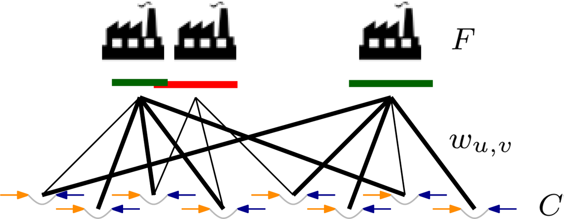
Let C be a set of clients and F be a set of facilities. Let \documentclass{aastex}\usepackage{amsbsy}\usepackage{amsfonts}\usepackage{amssymb}\usepackage{bm}\usepackage{mathrsfs}\usepackage{pifont}\usepackage{stmaryrd}\usepackage{textcomp}\usepackage{portland, xspace}\usepackage{amsmath, amsxtra}\pagestyle{empty}\DeclareMathSizes{10}{9}{7}{6}\begin{document} $$w : C {\times} F {\rightarrow} {\mathbb{R}}$$ \end{document} be the weight of assigning a given client to a given facility. Associated with every facility v ∈F, there is an interval I_v on the real line. We say that a subset of facilities S ⊆ F is independent if no two intervals in {I_v : v ∈S} overlap (see Fig. 2 for an example). We use P to denote the set of endpoints of all intervals.

FIG. 2.

Clients C and facilities F represent paired-end reads and candidate deletions, respectively. Each facility is associated with an interval whose endpoints correspond to the breakpoints of the candidate deletion. Edges between clients and facilities indicate alignments supporting the corresponding deletion. Our confidence in the alignment is captured by a score w. A feasible solution (bold edges) to the maximum facility location problem assigns reads to an independent set of facilities.

Finally, for any nonempty subset S ⊆ F we define the value of S as \documentclass{aastex}\usepackage{amsbsy}\usepackage{amsfonts}\usepackage{amssymb}\usepackage{bm}\usepackage{mathrsfs}\usepackage{pifont}\usepackage{stmaryrd}\usepackage{textcomp}\usepackage{portland, xspace}\usepackage{amsmath, amsxtra}\pagestyle{empty}\DeclareMathSizes{10}{9}{7}{6}\begin{document} \begin{align*}f ( S ) = \sum \limits_{u \in C} \max_{v \in S} w_{uv}. \tag{1}\end{align*} \end{document}

For completeness, we define \documentclass{aastex}\usepackage{amsbsy}\usepackage{amsfonts}\usepackage{amssymb}\usepackage{bm}\usepackage{mathrsfs}\usepackage{pifont}\usepackage{stmaryrd}\usepackage{textcomp}\usepackage{portland, xspace}\usepackage{amsmath, amsxtra}\pagestyle{empty}\DeclareMathSizes{10}{9}{7}{6}\begin{document} $$f ( \emptyset ) = 0$$ \end{document} .

An instance of the maximum facility location problem is specified by a tuple (C, F, w, I). The objective is to choose an independent subset S ⊆ F maximizing f (S). We now prove an important property about this objective function.

Definition 1. A function f is submodular if ∀A ⊆ B ⊆ F and ∀v ∈F\B \documentclass{aastex}\usepackage{amsbsy}\usepackage{amsfonts}\usepackage{amssymb}\usepackage{bm}\usepackage{mathrsfs}\usepackage{pifont}\usepackage{stmaryrd}\usepackage{textcomp}\usepackage{portland, xspace}\usepackage{amsmath, amsxtra}\pagestyle{empty}\DeclareMathSizes{10}{9}{7}{6}\begin{document} \begin{align*}f ( A + v ) - f ( A ) \ge f ( B + v ) - f ( B ).\end{align*} \end{document}

Lemma 1

The function f defined in (1) is monotone nondecreasing and submodular.

Proof. Let A ⊆ B ⊆ F. Notice that max_v′ ∈Aw_uv′ ≤ max_v′ ∈Bw_uv′ for all u ∈C. Summing over all u ∈C we get f (A) ≤ f (B). Therefore, f is monotone nondecreasing.

To prove the submodularity of f, consider a facility v ∈F\B. We add v to both A and B and analyze gain in value due to some arbitrary client u ∈C: \documentclass{aastex}\usepackage{amsbsy}\usepackage{amsfonts}\usepackage{amssymb}\usepackage{bm}\usepackage{mathrsfs}\usepackage{pifont}\usepackage{stmaryrd}\usepackage{textcomp}\usepackage{portland, xspace}\usepackage{amsmath, amsxtra}\pagestyle{empty}\DeclareMathSizes{10}{9}{7}{6}\begin{document} \begin{align} \max_{v^{ \prime} \in A + v} w_{uv^{ \prime}} - \max_{v^{ \prime} \in A} w_{uv^{ \prime}} & = \max ( 0 , w_{uv} - \max_{v^{ \prime} \in A} w_{uv^{ \prime}} ) , \\ & \ge \max ( 0 , w_{uv} - \max_{v^{ \prime} \in B} w_{uv^{ \prime}} ) = \max_{v^{ \prime} \in B + v} w_{uv^{ \prime}} - \max_{v^{ \prime} \in B} w_{uv^{ \prime}}.\end{align} \end{document}

Summing over all u ∈C we get f (A + v) − f (A) ≥ f (B + v) − f (B). Therefore, f is submodular. ■

2.1. Linear programming relaxation

Our linear programming relaxation (LP) uses two type of variables. For each facility v ∈F, we have a facility variable y_v that indicates whether facility v is open. For each client u ∈C and facility v ∈F, we have a client-facility variable x_uv that captures whether u is assigned to v.

The linear program has three types of constraints. For each client u∈C we have a constraint enforcing that u is assigned to at most one facility. For each client u∈C and facility v∈F we have a constraint enforcing that if u is assigned to v then v is open. Finally, for each interval endpoint p∈P we have a constraint enforcing that we choose at most one of the facilities whose intervals span p. \documentclass{aastex}\usepackage{amsbsy}\usepackage{amsfonts}\usepackage{amssymb}\usepackage{bm}\usepackage{mathrsfs}\usepackage{pifont}\usepackage{stmaryrd}\usepackage{textcomp}\usepackage{portland, xspace}\usepackage{amsmath, amsxtra}\pagestyle{empty}\DeclareMathSizes{10}{9}{7}{6}\begin{document} \begin{align} {\rm maximize} \mathop \sum \limits_{u \in C , v \in F} w_{uv} x_{uv}\end{align} \end{document} \documentclass{aastex}\usepackage{amsbsy}\usepackage{amsfonts}\usepackage{amssymb}\usepackage{bm}\usepackage{mathrsfs}\usepackage{pifont}\usepackage{stmaryrd}\usepackage{textcomp}\usepackage{portland, xspace}\usepackage{amsmath, amsxtra}\pagestyle{empty}\DeclareMathSizes{10}{9}{7}{6}\begin{document} \begin{align} \begin{split} { \rm subject \ to} \quad \mathop \sum \limits_{v \in F} x_{uv} &\leq 1 \quad \forall u \in C \\ x_{uv} &\leq y_v \ \ \forall u \in C , v \in F \\ \mathop \sum \limits_{v \in F : p \in I_v} y_{v} &\leq 1 \quad \forall p \in P \\ x_{uv} &\ge 0 \quad \forall u \in C , v \in F \\ y_v &\ge 0 \quad \forall v \in F\end{split} \tag{{ \rm LP}}\end{align} \end{document}

3. Algorithms

In this section we describe two algorithms for maximum facility location. Both algorithms solve the linear relaxation (LP) to get an optimal fractional solution and round it to a feasible integral solution using different approaches. The first algorithm uses independent rounding with alteration, while the second algorithm uses dependent rounding.

3.1. Independent rounding with alteration

Our first algorithm is very simple. First, we compute an optimal fractional solution (x, y) of the linear relaxation (LP). Then we create a set R ⊆ F by placing each facility v ∈F into R with probability αy_v, where α ∈[0, 1] is a parameter that will be chosen later to maximize the approximation ratio in our analysis. Finally, we apply a filtering step that drops some facilities so as to obtain an independent set T ⊆ R.

It should be noted that the alteration step (where we go from R to T) is the same as the conflict resolution scheme of Feldman (2013) that was developed for the more general problem of maximizing a submodular function subject to the constraint that the set chosen is independent in an auxiliary interval graph. As mentioned in the introduction, while this algorithm is a 0.25-approximation, it is not practical as it requires that we solve the stronger multilinear relaxation rather than the much easier linear relaxation (LP).

Algorithm 1:
Independent rounding with alterations.

function select-and-filter(α)

(x, y) ← solve (LP)

R ← Select each v∈F with probability αy_v

\documentclass{aastex}\usepackage{amsbsy}\usepackage{amsfonts}\usepackage{amssymb}\usepackage{bm}\usepackage{mathrsfs}\usepackage{pifont}\usepackage{stmaryrd}\usepackage{textcomp}\usepackage{portland, xspace}\usepackage{amsmath, amsxtra}\pagestyle{empty}\DeclareMathSizes{10}{9}{7}{6}\begin{document} $$ T \leftarrow \{ v \in R : \nexists v^{\prime} \in R \ {\rm such \ that \ start \ point \ of} \ I_v \ {\rm lies \ in} \ I_{v^{\prime}} \} $$ \end{document}

return T

The main result of this subsection is that this simple algorithm leads to a constant factor approximation.

Theorem 1

There is an LP-rounding 0.19-approximation for maximum facility location.

The proof of this theorem relies on a few auxiliary lemmas. First, we argue that solution T output is feasible. Then we argue that the expected value of the set R is at least a constant factor of the value of the fractional solution (x, y). Finally, we show that the expected value of T is at least a constant factor of the expected value of R.

Lemma 2

The set T returned by select-and-filter is independent.

Proof. Suppose, for the sake of contradiction, that T is not feasible. This means there are in T two facilities v and v′ whose intervals intersect. Without loss of generality assume that the start point of I_v is to the right of the start point of I_v_′. Since v′ ∈ T, it follows that v′ ∈ R. But then v should not belong in T since the start point of I_v lies in I_v_′, a contradiction. ■

Lemma 3

Let R be the set sampled by select-and-filter, then \documentclass{aastex}\usepackage{amsbsy}\usepackage{amsfonts}\usepackage{amssymb}\usepackage{bm}\usepackage{mathrsfs}\usepackage{pifont}\usepackage{stmaryrd}\usepackage{textcomp}\usepackage{portland, xspace}\usepackage{amsmath, amsxtra}\pagestyle{empty}\DeclareMathSizes{10}{9}{7}{6}\begin{document} \begin{align}{ \rm E} [ f ( R ) ] \ge ( 1 - e^{ - \alpha} ) \cdot \mathop \sum \limits_{u \in C , v \in F} w_{uv} \ x_{uv}.\end{align} \end{document}

Due to the technicality of the proof to Lemma 3, details are provided in Appendix A.

Lemma 4

Let R and T be the sets computed in select-and-filter then \documentclass{aastex}\usepackage{amsbsy}\usepackage{amsfonts}\usepackage{amssymb}\usepackage{bm}\usepackage{mathrsfs}\usepackage{pifont}\usepackage{stmaryrd}\usepackage{textcomp}\usepackage{portland, xspace}\usepackage{amsmath, amsxtra}\pagestyle{empty}\DeclareMathSizes{10}{9}{7}{6}\begin{document} \begin{align}{ \rm E} [ f ( T ) ] \ge ( 1 - \alpha ) \ { \rm E} [ f ( R ) ].\end{align} \end{document}

Proof. Let v ∈F and p be the start point of I_v. Let us start by estimating the probability that v ∉ T given that v ∈R. Recall that v is removed from R only if there exists v′ ∈ R such that p ∈I_v_′. Therefore, \documentclass{aastex}\usepackage{amsbsy}\usepackage{amsfonts}\usepackage{amssymb}\usepackage{bm}\usepackage{mathrsfs}\usepackage{pifont}\usepackage{stmaryrd}\usepackage{textcomp}\usepackage{portland, xspace}\usepackage{amsmath, amsxtra}\pagestyle{empty}\DeclareMathSizes{10}{9}{7}{6}\begin{document} \begin{align}{ \rm Pr} [ v \not \in T \mid v \in R ] = { \rm Pr} \left[ \bigvee_{{v^{ \prime} \in F - v: \atop p \in I_{v^{ \prime}}}} v^{ \prime} \in R \right] \leq \mathop \sum \limits_{v^{ \prime} \in F - v : \atop p \in I_{v^{ \prime}}} { \rm Pr} [ v^{ \prime} \in R ] = \mathop \sum \limits_{v^{ \prime} \in F - v: \atop p \in I_{v^{ \prime}}} \alpha y_{v^{ \prime}} \leq \alpha ,\end{align} \end{document}

where the first inequality follows from union bound, and the second from the feasibility of (x, y). Therefore, \documentclass{aastex}\usepackage{amsbsy}\usepackage{amsfonts}\usepackage{amssymb}\usepackage{bm}\usepackage{mathrsfs}\usepackage{pifont}\usepackage{stmaryrd}\usepackage{textcomp}\usepackage{portland, xspace}\usepackage{amsmath, amsxtra}\pagestyle{empty}\DeclareMathSizes{10}{9}{7}{6}\begin{document} \begin{align}{ \rm Pr} [ v \in T \mid v \in R ] \ge 1 - \alpha. \tag{2}\end{align} \end{document}

Vondrák et al. (2011, Theorem 1.3) showed⁴ that Equation (2) implies that \documentclass{aastex}\usepackage{amsbsy}\usepackage{amsfonts}\usepackage{amssymb}\usepackage{bm}\usepackage{mathrsfs}\usepackage{pifont}\usepackage{stmaryrd}\usepackage{textcomp}\usepackage{portland, xspace}\usepackage{amsmath, amsxtra}\pagestyle{empty}\DeclareMathSizes{10}{9}{7}{6}\begin{document} \begin{align}{ \rm E} [ f ( T ) ] \ge ( 1 - \alpha ) \ { \rm E} [ f ( R ) ] ,\end{align} \end{document}

when f is monotone submodular. From Lemma 1 we know that f is indeed monotone submodular. ■

Proof (of Theorem 1). Let R and T be the sets chosen by select-and-filter. By Lemma 2 the set T is independent. Its expected value is \documentclass{aastex}\usepackage{amsbsy}\usepackage{amsfonts}\usepackage{amssymb}\usepackage{bm}\usepackage{mathrsfs}\usepackage{pifont}\usepackage{stmaryrd}\usepackage{textcomp}\usepackage{portland, xspace}\usepackage{amsmath, amsxtra}\pagestyle{empty}\DeclareMathSizes{10}{9}{7}{6}\begin{document} \begin{align}{ \rm E} [ f ( T ) ] \ge ( 1 - \alpha ) \ { \rm E} [ f ( R ) ] \ge ( 1 - \alpha ) ( 1 - e^{ - \alpha} ) \mathop \sum \limits_{u \in C , v \in F} w_{uv} x_{uv} ,\end{align} \end{document}

where the first inequality follows from Lemma 4 and the second inequality from Lemma 3.

The best approximation ratio is attained at α = 0.44, where we get 0.199. ■

Algorithm engineering. We briefly discuss two ideas for improving the observed performance of select-and-filter without sacrificing its theoretical guarantees: Picking the optimal α and resolve conflicts less aggressively.

First, notice that our choice of α in the proof of Theorem 1 may not be the best for a particular instance. Instead of picking a single value of α we pick the “best” α as follows. For each v ∈F, we generate a random number r_v ∈[0, 1). In select-and-filter, we can think of a facility v being added to the set R if r_v ≤ αy_v. Therefore there are discrete values of α for which we add a new facility v to our set R. Let R_α = {v ∈F : r_v ≤ αy_v} and \documentclass{aastex}\usepackage{amsbsy}\usepackage{amsfonts}\usepackage{amssymb}\usepackage{bm}\usepackage{mathrsfs}\usepackage{pifont}\usepackage{stmaryrd}\usepackage{textcomp}\usepackage{portland, xspace}\usepackage{amsmath, amsxtra}\pagestyle{empty}\DeclareMathSizes{10}{9}{7}{6}\begin{document} $$\alpha_1 < \alpha_2 < \cdots < \alpha_n$$ \end{document} be the interesting values of α when R_α changes; that is, α_j = r_v/y_v for some v ∈F. Observe that \documentclass{aastex}\usepackage{amsbsy}\usepackage{amsfonts}\usepackage{amssymb}\usepackage{bm}\usepackage{mathrsfs}\usepackage{pifont}\usepackage{stmaryrd}\usepackage{textcomp}\usepackage{portland, xspace}\usepackage{amsmath, amsxtra}\pagestyle{empty}\DeclareMathSizes{10}{9}{7}{6}\begin{document} $$R_{ \alpha_1} \subset R_{ \alpha_2} \subset \cdots \subset R_{ \alpha_n}$$ \end{document} . Then we can simply compute T_{α_i} for each value of α_i and return the set maximizing f (T_{α_i}).

Second, recall that the algorithm resolves conflicts of R by keeping only those facilities whose start point is not contained in another interval in R. Consider a maximal subset A ⊆ R such that the union of their intervals forms a single interval. For each such A, the filtering step of select-and-filter would only place the facility in A with the leftmost start point into T. Instead, we can be less aggressive and pick a maximal independent subset of A that includes the leftmost interval. Thus, we are guaranteed to pick an independent set that is a superset of the set chosen by the simple version.

3.2. Dependent rounding

Our second algorithm uses a more refined rounding routine. Instead of sampling and removing intervals that have conflicts, we gradually shift the fractional solution to an integral using dependent rounding (Gandhi et al., 2006) routine.

Before we can describe the algorithm we need a few definitions. Given a solution (x, y) to (LP), let S = {v ∈F : 0 < y_v < 1} be the set of facilities with a nonintegral value. For a point p∈P, let slack(p) denote the slack of its corresponding constraint in (LP): \documentclass{aastex}\usepackage{amsbsy}\usepackage{amsfonts}\usepackage{amssymb}\usepackage{bm}\usepackage{mathrsfs}\usepackage{pifont}\usepackage{stmaryrd}\usepackage{textcomp}\usepackage{portland, xspace}\usepackage{amsmath, amsxtra}\pagestyle{empty}\DeclareMathSizes{10}{9}{7}{6}\begin{document} \begin{align}{ \rm slack} ( p ) = 1 - \mathop \sum \limits_{v \in F: p \in I_v} y_v.\end{align} \end{document}

We say p is tight if its constraint is tight; namely, if slack(p) = 0.

Our algorithm starts by finding an optimal fractional solution (x, y) to the linear relaxation (LP). Then we iteratively modify this solution as follows. First, we select two disjoint independent subsets M₁, M₂ ⊂ S. Then, we randomly update the y-values of facilities in M₁ ∪ M₂ so that at least one more facility is integral or at least one more point is tight. This is repeated until there are no more fractionally opened facilities.

Let us describe in more detail how the update is carried out. For i = 1, 2, let P_i ⊆ P be those points that intersect an interval in M_i. We compute the following two quantities \documentclass{aastex}\usepackage{amsbsy}\usepackage{amsfonts}\usepackage{amssymb}\usepackage{bm}\usepackage{mathrsfs}\usepackage{pifont}\usepackage{stmaryrd}\usepackage{textcomp}\usepackage{portland, xspace}\usepackage{amsmath, amsxtra}\pagestyle{empty}\DeclareMathSizes{10}{9}{7}{6}\begin{document} \begin{align} & \varepsilon = \min \left( \min_{p \in P_1 \backslash P_2} { \rm slack} ( p ) , \min_{v \in M_2} y_v \right) , \\ & \delta = \min \left( \min_{p \in P_2 \backslash P_1} { \rm slack} ( p ) , \min_{v \in M_1} y_v \right) .\end{align} \end{document}

Finally, with probability \documentclass{aastex}\usepackage{amsbsy}\usepackage{amsfonts}\usepackage{amssymb}\usepackage{bm}\usepackage{mathrsfs}\usepackage{pifont}\usepackage{stmaryrd}\usepackage{textcomp}\usepackage{portland, xspace}\usepackage{amsmath, amsxtra}\pagestyle{empty}\DeclareMathSizes{10}{9}{7}{6}\begin{document} $$ \frac { \varepsilon } { \varepsilon + \delta } $$ \end{document} we replace the current fractional solution y with a new solution \documentclass{aastex}\usepackage{amsbsy}\usepackage{amsfonts}\usepackage{amssymb}\usepackage{bm}\usepackage{mathrsfs}\usepackage{pifont}\usepackage{stmaryrd}\usepackage{textcomp}\usepackage{portland, xspace}\usepackage{amsmath, amsxtra}\pagestyle{empty}\DeclareMathSizes{10}{9}{7}{6}\begin{document} \begin{align}y^{ \prime}_v = \begin{cases}y_v - \delta , \quad v \in M_1 , \\ y_v + \delta , \quad v \in M_2 , \\ y_v , \quad { \rm otherwise}.\end{cases}\end{align} \end{document}

Otherwise, with complementary probability \documentclass{aastex}\usepackage{amsbsy}\usepackage{amsfonts}\usepackage{amssymb}\usepackage{bm}\usepackage{mathrsfs}\usepackage{pifont}\usepackage{stmaryrd}\usepackage{textcomp}\usepackage{portland, xspace}\usepackage{amsmath, amsxtra}\pagestyle{empty}\DeclareMathSizes{10}{9}{7}{6}\begin{document} $$ \frac { \delta } { \varepsilon + \delta } $$ \end{document} , we replace y with the new solution \documentclass{aastex}\usepackage{amsbsy}\usepackage{amsfonts}\usepackage{amssymb}\usepackage{bm}\usepackage{mathrsfs}\usepackage{pifont}\usepackage{stmaryrd}\usepackage{textcomp}\usepackage{portland, xspace}\usepackage{amsmath, amsxtra}\pagestyle{empty}\DeclareMathSizes{10}{9}{7}{6}\begin{document} \begin{align}y^{ \prime \prime}_v = \begin{cases}y_v + \varepsilon , \quad v \in M_1 , \\ y_v - \varepsilon , \quad v \in M_2 , \\ y_v , \quad { \rm otherwise}.\end{cases}\end{align} \end{document}

The pseudocode of the main routine is given in Algorithm 2, while the pseudocode for picking M₁ and M₂ appears in Algorithm 3.

The following Theorem is the main result of this section.

Theorem 2

Let T be the set returned by dependent-rounding. Then T is independent and Pr[v ∈T] = y_v for all v ∈F.

Algorithm 3:
Creating subsets M₁ and M₂.

function select-subsets(S, y)

\documentclass{aastex}\usepackage{amsbsy}\usepackage{amsfonts}\usepackage{amssymb}\usepackage{bm}\usepackage{mathrsfs}\usepackage{pifont}\usepackage{stmaryrd}\usepackage{textcomp}\usepackage{portland, xspace}\usepackage{amsmath, amsxtra}\pagestyle{empty}\DeclareMathSizes{10}{9}{7}{6}\begin{document} $$\tilde{P}$$ \end{document} ← the set of tight points in S sorted from left to right

v₁ ← a facility in S whose interval has leftmost start point

v₂ ← a facility in S–v₁ whose interval starts at the first tight point in \documentclass{aastex}\usepackage{amsbsy}\usepackage{amsfonts}\usepackage{amssymb}\usepackage{bm}\usepackage{mathrsfs}\usepackage{pifont}\usepackage{stmaryrd}\usepackage{textcomp}\usepackage{portland, xspace}\usepackage{amsmath, amsxtra}\pagestyle{empty}\DeclareMathSizes{10}{9}{7}{6}\begin{document} $$\tilde{P}$$ \end{document}

M₁ ←{v₁}

M₂ ←{v₂}

for every tight point t in \documentclass{aastex}\usepackage{amsbsy}\usepackage{amsfonts}\usepackage{amssymb}\usepackage{bm}\usepackage{mathrsfs}\usepackage{pifont}\usepackage{stmaryrd}\usepackage{textcomp}\usepackage{portland, xspace}\usepackage{amsmath, amsxtra}\pagestyle{empty}\DeclareMathSizes{10}{9}{7}{6}\begin{document} $$\tilde{P}$$ \end{document} (in sorted order) do

if \documentclass{aastex}\usepackage{amsbsy}\usepackage{amsfonts}\usepackage{amssymb}\usepackage{bm}\usepackage{mathrsfs}\usepackage{pifont}\usepackage{stmaryrd}\usepackage{textcomp}\usepackage{portland, xspace}\usepackage{amsmath, amsxtra}\pagestyle{empty}\DeclareMathSizes{10}{9}{7}{6}\begin{document} $$I_{v_1}$$ \end{document} contains t and \documentclass{aastex}\usepackage{amsbsy}\usepackage{amsfonts}\usepackage{amssymb}\usepackage{bm}\usepackage{mathrsfs}\usepackage{pifont}\usepackage{stmaryrd}\usepackage{textcomp}\usepackage{portland, xspace}\usepackage{amsmath, amsxtra}\pagestyle{empty}\DeclareMathSizes{10}{9}{7}{6}\begin{document} $$I_{v_2}$$ \end{document} contains t then

continue

v ← the facility in S starting at t

if \documentclass{aastex}\usepackage{amsbsy}\usepackage{amsfonts}\usepackage{amssymb}\usepackage{bm}\usepackage{mathrsfs}\usepackage{pifont}\usepackage{stmaryrd}\usepackage{textcomp}\usepackage{portland, xspace}\usepackage{amsmath, amsxtra}\pagestyle{empty}\DeclareMathSizes{10}{9}{7}{6}\begin{document} $$I_{v_2}$$ \end{document} contains t then

Add v to M₁

v₁ ← v

else if \documentclass{aastex}\usepackage{amsbsy}\usepackage{amsfonts}\usepackage{amssymb}\usepackage{bm}\usepackage{mathrsfs}\usepackage{pifont}\usepackage{stmaryrd}\usepackage{textcomp}\usepackage{portland, xspace}\usepackage{amsmath, amsxtra}\pagestyle{empty}\DeclareMathSizes{10}{9}{7}{6}\begin{document} $$I_{v_1}$$ \end{document} contains t then

Add v to M₂

v₂ ← v

else

break

return M₁, M₂

We break the analysis into a series of lemmas. First, we prove some properties of the output of select-subsets. Then, we prove that the expected value of the fractional solution at the end of an iteration equals its value at the beginning of the iteration. Finally, we show that in each iteration we either gain an additional integral facility or a new tight point.

Lemma 5

Let M₁ and M₂ be the sets computed by select-subsets. Then M₁ and M₂ are disjoint and both are independent. Furthermore, if p ∈P is a tight point then either p stabs both M₁ and M₂, or none of them.

Proof. Observe that every tight point must occur at an interval start point. Let v₁ be the facility whose interval I_v₁ is the first in S (from left to right). If the first tight point is to the right of the start point of \documentclass{aastex}\usepackage{amsbsy}\usepackage{amsfonts}\usepackage{amssymb}\usepackage{bm}\usepackage{mathrsfs}\usepackage{pifont}\usepackage{stmaryrd}\usepackage{textcomp}\usepackage{portland, xspace}\usepackage{amsmath, amsxtra}\pagestyle{empty}\DeclareMathSizes{10}{9}{7}{6}\begin{document} $$I_{v_1}$$ \end{document} then \documentclass{aastex}\usepackage{amsbsy}\usepackage{amsfonts}\usepackage{amssymb}\usepackage{bm}\usepackage{mathrsfs}\usepackage{pifont}\usepackage{stmaryrd}\usepackage{textcomp}\usepackage{portland, xspace}\usepackage{amsmath, amsxtra}\pagestyle{empty}\DeclareMathSizes{10}{9}{7}{6}\begin{document} $$I_{v_2}$$ \end{document} is welldefined. Otherwise, if the start point of \documentclass{aastex}\usepackage{amsbsy}\usepackage{amsfonts}\usepackage{amssymb}\usepackage{bm}\usepackage{mathrsfs}\usepackage{pifont}\usepackage{stmaryrd}\usepackage{textcomp}\usepackage{portland, xspace}\usepackage{amsmath, amsxtra}\pagestyle{empty}\DeclareMathSizes{10}{9}{7}{6}\begin{document} $$I_{v_1}$$ \end{document} is tight there must be another facility starting at that point (since S is the set of nonintegral facilities) so \documentclass{aastex}\usepackage{amsbsy}\usepackage{amsfonts}\usepackage{amssymb}\usepackage{bm}\usepackage{mathrsfs}\usepackage{pifont}\usepackage{stmaryrd}\usepackage{textcomp}\usepackage{portland, xspace}\usepackage{amsmath, amsxtra}\pagestyle{empty}\DeclareMathSizes{10}{9}{7}{6}\begin{document} $$I_{v_2}$$ \end{document} is welldefined in this case too.

Now that we have shown the invariant holds after initialization, we aim to prove that M₁ and M₂ are independent. To do this, we need to show that the loop invariant also holds at the end of each iteration. Consider the next tight point t and facility v starting at t. Suppose t stabs \documentclass{aastex}\usepackage{amsbsy}\usepackage{amsfonts}\usepackage{amssymb}\usepackage{bm}\usepackage{mathrsfs}\usepackage{pifont}\usepackage{stmaryrd}\usepackage{textcomp}\usepackage{portland, xspace}\usepackage{amsmath, amsxtra}\pagestyle{empty}\DeclareMathSizes{10}{9}{7}{6}\begin{document} $$I_{v_2}$$ \end{document} only but it does not stab \documentclass{aastex}\usepackage{amsbsy}\usepackage{amsfonts}\usepackage{amssymb}\usepackage{bm}\usepackage{mathrsfs}\usepackage{pifont}\usepackage{stmaryrd}\usepackage{textcomp}\usepackage{portland, xspace}\usepackage{amsmath, amsxtra}\pagestyle{empty}\DeclareMathSizes{10}{9}{7}{6}\begin{document} $$I_{v_1}$$ \end{document} . Since we scan from left to right, \documentclass{aastex}\usepackage{amsbsy}\usepackage{amsfonts}\usepackage{amssymb}\usepackage{bm}\usepackage{mathrsfs}\usepackage{pifont}\usepackage{stmaryrd}\usepackage{textcomp}\usepackage{portland, xspace}\usepackage{amsmath, amsxtra}\pagestyle{empty}\DeclareMathSizes{10}{9}{7}{6}\begin{document} $$I_{v_1}$$ \end{document} is to the left of t and I_v starts at t, as shown in Figure 3. Therefore, we can add v to M₁ correctly and update v₁ = v. The case when t stabs \documentclass{aastex}\usepackage{amsbsy}\usepackage{amsfonts}\usepackage{amssymb}\usepackage{bm}\usepackage{mathrsfs}\usepackage{pifont}\usepackage{stmaryrd}\usepackage{textcomp}\usepackage{portland, xspace}\usepackage{amsmath, amsxtra}\pagestyle{empty}\DeclareMathSizes{10}{9}{7}{6}\begin{document} $$I_{v_1}$$ \end{document} but not \documentclass{aastex}\usepackage{amsbsy}\usepackage{amsfonts}\usepackage{amssymb}\usepackage{bm}\usepackage{mathrsfs}\usepackage{pifont}\usepackage{stmaryrd}\usepackage{textcomp}\usepackage{portland, xspace}\usepackage{amsmath, amsxtra}\pagestyle{empty}\DeclareMathSizes{10}{9}{7}{6}\begin{document} $$I_{v_2}$$ \end{document} is handled in a similar fashion, but adding v to M₂ and updating v₂ = v. Finally, if t stabs both \documentclass{aastex}\usepackage{amsbsy}\usepackage{amsfonts}\usepackage{amssymb}\usepackage{bm}\usepackage{mathrsfs}\usepackage{pifont}\usepackage{stmaryrd}\usepackage{textcomp}\usepackage{portland, xspace}\usepackage{amsmath, amsxtra}\pagestyle{empty}\DeclareMathSizes{10}{9}{7}{6}\begin{document} $$I_{v_1}$$ \end{document} and \documentclass{aastex}\usepackage{amsbsy}\usepackage{amsfonts}\usepackage{amssymb}\usepackage{bm}\usepackage{mathrsfs}\usepackage{pifont}\usepackage{stmaryrd}\usepackage{textcomp}\usepackage{portland, xspace}\usepackage{amsmath, amsxtra}\pagestyle{empty}\DeclareMathSizes{10}{9}{7}{6}\begin{document} $$I_{v_2}$$ \end{document} , we continue to the next tight point; otherwise, if t stabs neither \documentclass{aastex}\usepackage{amsbsy}\usepackage{amsfonts}\usepackage{amssymb}\usepackage{bm}\usepackage{mathrsfs}\usepackage{pifont}\usepackage{stmaryrd}\usepackage{textcomp}\usepackage{portland, xspace}\usepackage{amsmath, amsxtra}\pagestyle{empty}\DeclareMathSizes{10}{9}{7}{6}\begin{document} $$I_{v_1}$$ \end{document} or \documentclass{aastex}\usepackage{amsbsy}\usepackage{amsfonts}\usepackage{amssymb}\usepackage{bm}\usepackage{mathrsfs}\usepackage{pifont}\usepackage{stmaryrd}\usepackage{textcomp}\usepackage{portland, xspace}\usepackage{amsmath, amsxtra}\pagestyle{empty}\DeclareMathSizes{10}{9}{7}{6}\begin{document} $$I_{v_2}$$ \end{document} , the algorithm stops. Clearly there are a finite number of tight points; therefore, the loop will eventually terminate. Consequently, the invariant holds throughout.

FIG. 3.
The case when only one of the intervals stabs the next tight point.

Now consider a tight point p ∈P. If p was never considered by the for loop, then p∉ \documentclass{aastex}\usepackage{amsbsy}\usepackage{amsfonts}\usepackage{amssymb}\usepackage{bm}\usepackage{mathrsfs}\usepackage{pifont}\usepackage{stmaryrd}\usepackage{textcomp}\usepackage{portland, xspace}\usepackage{amsmath, amsxtra}\pagestyle{empty}\DeclareMathSizes{10}{9}{7}{6}\begin{document} $$\tilde{P}$$ \end{document} and thus is strictly to the right or to the left of every interval in M₁ ∪ M₂, and thus does not stab any of them. Otherwise, in the iteration when p was considered by the algorithm it either intersected both \documentclass{aastex}\usepackage{amsbsy}\usepackage{amsfonts}\usepackage{amssymb}\usepackage{bm}\usepackage{mathrsfs}\usepackage{pifont}\usepackage{stmaryrd}\usepackage{textcomp}\usepackage{portland, xspace}\usepackage{amsmath, amsxtra}\pagestyle{empty}\DeclareMathSizes{10}{9}{7}{6}\begin{document} $$I_{v_1}$$ \end{document} and \documentclass{aastex}\usepackage{amsbsy}\usepackage{amsfonts}\usepackage{amssymb}\usepackage{bm}\usepackage{mathrsfs}\usepackage{pifont}\usepackage{stmaryrd}\usepackage{textcomp}\usepackage{portland, xspace}\usepackage{amsmath, amsxtra}\pagestyle{empty}\DeclareMathSizes{10}{9}{7}{6}\begin{document} $$I_{v_2}$$ \end{document} , in which case we are done, or it added v so that the property holds. ■

Lemma 6

Consider an iteration of dependent-rounding. Let y be the fractional solution at the beginning, and \documentclass{aastex}\usepackage{amsbsy}\usepackage{amsfonts}\usepackage{amssymb}\usepackage{bm}\usepackage{mathrsfs}\usepackage{pifont}\usepackage{stmaryrd}\usepackage{textcomp}\usepackage{portland, xspace}\usepackage{amsmath, amsxtra}\pagestyle{empty}\DeclareMathSizes{10}{9}{7}{6}\begin{document} $$\hat{y}$$ \end{document} be the solution at the end of the iteration. Then for every v∈F we have \documentclass{aastex}\usepackage{amsbsy}\usepackage{amsfonts}\usepackage{amssymb}\usepackage{bm}\usepackage{mathrsfs}\usepackage{pifont}\usepackage{stmaryrd}\usepackage{textcomp}\usepackage{portland, xspace}\usepackage{amsmath, amsxtra}\pagestyle{empty}\DeclareMathSizes{10}{9}{7}{6}\begin{document} $${ \rm E} [ \hat y_v ] = y_v$$ \end{document} . Furthermore, \documentclass{aastex}\usepackage{amsbsy}\usepackage{amsfonts}\usepackage{amssymb}\usepackage{bm}\usepackage{mathrsfs}\usepackage{pifont}\usepackage{stmaryrd}\usepackage{textcomp}\usepackage{portland, xspace}\usepackage{amsmath, amsxtra}\pagestyle{empty}\DeclareMathSizes{10}{9}{7}{6}\begin{document} $$\hat{y}$$ \end{document} obeys the independence and non-negativity constraints of (LP).

Proof. If we have a facility v ∈F that is not in M₁ or M₂, then it is clear that the equality holds as its value does not change. For each facility v∉M₁ we have \documentclass{aastex}\usepackage{amsbsy}\usepackage{amsfonts}\usepackage{amssymb}\usepackage{bm}\usepackage{mathrsfs}\usepackage{pifont}\usepackage{stmaryrd}\usepackage{textcomp}\usepackage{portland, xspace}\usepackage{amsmath, amsxtra}\pagestyle{empty}\DeclareMathSizes{10}{9}{7}{6}\begin{document} \begin{align} { \rm E } [ \hat { y } _v ] & = \left( \frac { \varepsilon } { \varepsilon + \delta } \right) ( y_v - \delta ) + \left( \frac { \delta } { \varepsilon + \delta } \right) ( y_v + \varepsilon ) \\ & = \frac { \varepsilon y_v - \varepsilon \delta + \delta y_v + \varepsilon \delta } { \varepsilon + \delta } \\ & = y_v. \end{align} \end{document}

A similar argument applies for facilities v ∈M₂.

Notice that \documentclass{aastex}\usepackage{amsbsy}\usepackage{amsfonts}\usepackage{amssymb}\usepackage{bm}\usepackage{mathrsfs}\usepackage{pifont}\usepackage{stmaryrd}\usepackage{textcomp}\usepackage{portland, xspace}\usepackage{amsmath, amsxtra}\pagestyle{empty}\DeclareMathSizes{10}{9}{7}{6}\begin{document} $$\hat {y}_v \ge 0$$ \end{document} by our definition of ɛ and δ since each of these values is less than or equal to the minimum y-value of the subset of variables that are decreased in each case.

Finally, let us now argue that y obeys the independence constraints of (LP). Let p ∈P be an arbitrary point. If p ∈P₁∩P₂ then its constraint is obeyed since the increase/decrease of a facility in M₁ that it stabs is compensated with a corresponding decrease/increase of a facility in M₂ that it stabs. If p ∈P₁\P₂ then by the definition of ɛ the independence constraint at p is obeyed. Similarly, if p ∈P₂\P₁ then by the definition of δ the independence constraint at p is obeyed. Finally, p ∉P₁ ∪ P₂ then the slack of p does not change so the independence constraint at p is obeyed as well. ■

Lemma 7

In each iteration of dependent-rounding we either gain a new integral facility or a new tight point.

Proof. Let us argue that ɛ > 0 and δ > 0. Note that min_v ∈M2y_v > 0 since all facilities in M₂ are nonintegral, and that min _p ∈P1\P2 slack(p) > 0 since all tight points that stab M₁ also stab M₂. Putting these two facts together, we get ɛ > 0. A similar line of reasoning yields δ > 0. Therefore, no matter what type of update we perform, we always move to a different fractional solution.

Suppose that the algorithm replaces y with y′. Furthermore, assume that ɛ = y_v for some v ∈M₂. It follows that \documentclass{aastex}\usepackage{amsbsy}\usepackage{amsfonts}\usepackage{amssymb}\usepackage{bm}\usepackage{mathrsfs}\usepackage{pifont}\usepackage{stmaryrd}\usepackage{textcomp}\usepackage{portland, xspace}\usepackage{amsmath, amsxtra}\pagestyle{empty}\DeclareMathSizes{10}{9}{7}{6}\begin{document} $$y^{ \prime}_v = 0$$ \end{document} , so we gain a new integral facility. Similarly, assume that ɛ = slack(p) for some p ∈P₁\P₂. After the update the slack at p will be 0, so we gain a new tight point since by Lemma 5 the point p cannot be tight. Therefore, either y′ has one additional integral facility, or one additional tight point. A similar argument shows that the same holds if the algorithm decides to replace y with y′′. ■

Proof (of Theorem 2). By Lemma 7, in each iteration we either gain one additional integral facility or one additional tight point. Therefore, after 2|F| iterations the algorithm must terminate with an integral solution \documentclass{aastex}\usepackage{amsbsy}\usepackage{amsfonts}\usepackage{amssymb}\usepackage{bm}\usepackage{mathrsfs}\usepackage{pifont}\usepackage{stmaryrd}\usepackage{textcomp}\usepackage{portland, xspace}\usepackage{amsmath, amsxtra}\pagestyle{empty}\DeclareMathSizes{10}{9}{7}{6}\begin{document} $${ \hat {y}}$$ \end{document} .

By Lemma 6, in each iteration we maintain feasibility. It follows that the set \documentclass{aastex}\usepackage{amsbsy}\usepackage{amsfonts}\usepackage{amssymb}\usepackage{bm}\usepackage{mathrsfs}\usepackage{pifont}\usepackage{stmaryrd}\usepackage{textcomp}\usepackage{portland, xspace}\usepackage{amsmath, amsxtra}\pagestyle{empty}\DeclareMathSizes{10}{9}{7}{6}\begin{document} $$T = \{ v \in F : \hat {y}_v = 1 \} $$ \end{document} is feasible. Finally, by Lemma 6 and induction we get Pr[v ∈T] = y_v for all v ∈F. ■

In terms of the differences between these two algorithms discussed, they both exhibit a trade-off in solution quality versus time. The first algorithm (independent rounding) presented has a theoretical bound, however will often be slower than the second; as for large instances we need to evaluate the objective function in Equation (1) many times. On the other hand, the runtime of the second algorithm (dependent rounding) is dependent on the number of tight points in the instance. Therefore for instances with a small number of tight points, the dependent algorithm will most likely have a faster running time.

We close this section by noting that while the output set T is independent and Pr[v ∈T] = y_v, we cannot prove the guarantee of Lemma 3 for E[f (T)] since the rounding decisions are not independent of one another.

4. Hardness

In this section we discuss the inapproximability of maximum facility location. In particular, we show that there is no polynomial time α-approximation for α > (1 − 1/e) unless P = NP.

Theorem 3

For any ɛ > 0, there is no (1 − 1/e+ɛ)-approximation algorithm for maximum facility location, unless P = NP.

Proof. In order to show hardness of the maximum facility location problem, we reduce it from the maximum coverage problem. In the maximum coverage problem we are given an integer k, a universe \documentclass{aastex}\usepackage{amsbsy}\usepackage{amsfonts}\usepackage{amssymb}\usepackage{bm}\usepackage{mathrsfs}\usepackage{pifont}\usepackage{stmaryrd}\usepackage{textcomp}\usepackage{portland, xspace}\usepackage{amsmath, amsxtra}\pagestyle{empty}\DeclareMathSizes{10}{9}{7}{6}\begin{document} $${ {\cal U}} = \{ u_1 , u_2 , \ldots , u_n \} $$ \end{document} , and a collection of subsets \documentclass{aastex}\usepackage{amsbsy}\usepackage{amsfonts}\usepackage{amssymb}\usepackage{bm}\usepackage{mathrsfs}\usepackage{pifont}\usepackage{stmaryrd}\usepackage{textcomp}\usepackage{portland, xspace}\usepackage{amsmath, amsxtra}\pagestyle{empty}\DeclareMathSizes{10}{9}{7}{6}\begin{document} $${ {\cal S}} = \{ S_1 , S_2 , \ldots , S_m \} $$ \end{document} such that \documentclass{aastex}\usepackage{amsbsy}\usepackage{amsfonts}\usepackage{amssymb}\usepackage{bm}\usepackage{mathrsfs}\usepackage{pifont}\usepackage{stmaryrd}\usepackage{textcomp}\usepackage{portland, xspace}\usepackage{amsmath, amsxtra}\pagestyle{empty}\DeclareMathSizes{10}{9}{7}{6}\begin{document} $$\forall S \in { {\cal S}} : S \subseteq { {\cal U}}$$ \end{document} . Our goal is to select a collection \documentclass{aastex}\usepackage{amsbsy}\usepackage{amsfonts}\usepackage{amssymb}\usepackage{bm}\usepackage{mathrsfs}\usepackage{pifont}\usepackage{stmaryrd}\usepackage{textcomp}\usepackage{portland, xspace}\usepackage{amsmath, amsxtra}\pagestyle{empty}\DeclareMathSizes{10}{9}{7}{6}\begin{document} $${ {\cal C}} \subseteq { {\cal S}}$$ \end{document} of these subsets, where \documentclass{aastex}\usepackage{amsbsy}\usepackage{amsfonts}\usepackage{amssymb}\usepackage{bm}\usepackage{mathrsfs}\usepackage{pifont}\usepackage{stmaryrd}\usepackage{textcomp}\usepackage{portland, xspace}\usepackage{amsmath, amsxtra}\pagestyle{empty}\DeclareMathSizes{10}{9}{7}{6}\begin{document} $$\mid { {\cal C}} \mid \leq k$$ \end{document} , and we maximize the quantity \documentclass{aastex}\usepackage{amsbsy}\usepackage{amsfonts}\usepackage{amssymb}\usepackage{bm}\usepackage{mathrsfs}\usepackage{pifont}\usepackage{stmaryrd}\usepackage{textcomp}\usepackage{portland, xspace}\usepackage{amsmath, amsxtra}\pagestyle{empty}\DeclareMathSizes{10}{9}{7}{6}\begin{document} \begin{align} \left|\bigcup \limits_{S_i \in { {\cal C}}} S_i \right|. \end{align} \end{document}

It has been shown that there is no polynomial time algorithm for this problem with an α-approximation for \documentclass{aastex}\usepackage{amsbsy}\usepackage{amsfonts}\usepackage{amssymb}\usepackage{bm}\usepackage{mathrsfs}\usepackage{pifont}\usepackage{stmaryrd}\usepackage{textcomp}\usepackage{portland, xspace}\usepackage{amsmath, amsxtra}\pagestyle{empty}\DeclareMathSizes{10}{9}{7}{6}\begin{document} $$\alpha > \left( 1 - \frac { 1 } { e } \right)$$ \end{document} unless P = NP (Feige, 1998; Khuller et al., 1999).

To begin the reduction to maximum facility location, we create a client c_u for each element \documentclass{aastex}\usepackage{amsbsy}\usepackage{amsfonts}\usepackage{amssymb}\usepackage{bm}\usepackage{mathrsfs}\usepackage{pifont}\usepackage{stmaryrd}\usepackage{textcomp}\usepackage{portland, xspace}\usepackage{amsmath, amsxtra}\pagestyle{empty}\DeclareMathSizes{10}{9}{7}{6}\begin{document} $$u \in { {\cal U}}$$ \end{document} . The main constraint we model is that we can only pick at most k subsets from our collection \documentclass{aastex}\usepackage{amsbsy}\usepackage{amsfonts}\usepackage{amssymb}\usepackage{bm}\usepackage{mathrsfs}\usepackage{pifont}\usepackage{stmaryrd}\usepackage{textcomp}\usepackage{portland, xspace}\usepackage{amsmath, amsxtra}\pagestyle{empty}\DeclareMathSizes{10}{9}{7}{6}\begin{document} $${ {\cal S}}$$ \end{document} . Therefore we create \documentclass{aastex}\usepackage{amsbsy}\usepackage{amsfonts}\usepackage{amssymb}\usepackage{bm}\usepackage{mathrsfs}\usepackage{pifont}\usepackage{stmaryrd}\usepackage{textcomp}\usepackage{portland, xspace}\usepackage{amsmath, amsxtra}\pagestyle{empty}\DeclareMathSizes{10}{9}{7}{6}\begin{document} $$k \mid { {\cal S}} \mid$$ \end{document} facilities. For each subset \documentclass{aastex}\usepackage{amsbsy}\usepackage{amsfonts}\usepackage{amssymb}\usepackage{bm}\usepackage{mathrsfs}\usepackage{pifont}\usepackage{stmaryrd}\usepackage{textcomp}\usepackage{portland, xspace}\usepackage{amsmath, amsxtra}\pagestyle{empty}\DeclareMathSizes{10}{9}{7}{6}\begin{document} $$S \in { {\cal S}}$$ \end{document} , we create the facilities φ_S,₁, φ_S,₂,…, φ_S,k representing the subset S. From these facilities, we form k cliques in the interval graph such that for every value of i ∈[1, k], every pair of intervals in the set \documentclass{aastex}\usepackage{amsbsy}\usepackage{amsfonts}\usepackage{amssymb}\usepackage{bm}\usepackage{mathrsfs}\usepackage{pifont}\usepackage{stmaryrd}\usepackage{textcomp}\usepackage{portland, xspace}\usepackage{amsmath, amsxtra}\pagestyle{empty}\DeclareMathSizes{10}{9}{7}{6}\begin{document} $$\{ I_{ \phi_{S , i}} \mid S \in { {\cal S}} \} $$ \end{document} is overlapping. This ensures that we can only choose to open one facility (i.e., select one subset from the collection) from each clique, and this can be done at most k times.

If an element \documentclass{aastex}\usepackage{amsbsy}\usepackage{amsfonts}\usepackage{amssymb}\usepackage{bm}\usepackage{mathrsfs}\usepackage{pifont}\usepackage{stmaryrd}\usepackage{textcomp}\usepackage{portland, xspace}\usepackage{amsmath, amsxtra}\pagestyle{empty}\DeclareMathSizes{10}{9}{7}{6}\begin{document} $$u \in { {\cal U}}$$ \end{document} is in a set \documentclass{aastex}\usepackage{amsbsy}\usepackage{amsfonts}\usepackage{amssymb}\usepackage{bm}\usepackage{mathrsfs}\usepackage{pifont}\usepackage{stmaryrd}\usepackage{textcomp}\usepackage{portland, xspace}\usepackage{amsmath, amsxtra}\pagestyle{empty}\DeclareMathSizes{10}{9}{7}{6}\begin{document} $$S \in { {\cal S}}$$ \end{document} , then we add the edges \documentclass{aastex}\usepackage{amsbsy}\usepackage{amsfonts}\usepackage{amssymb}\usepackage{bm}\usepackage{mathrsfs}\usepackage{pifont}\usepackage{stmaryrd}\usepackage{textcomp}\usepackage{portland, xspace}\usepackage{amsmath, amsxtra}\pagestyle{empty}\DeclareMathSizes{10}{9}{7}{6}\begin{document} \begin{align}( c_u , \phi_{S , 1} ) , ( c_u , \phi_{S , 2} ) , \ldots , ( c_u , \phi_{S , k} )\end{align} \end{document}

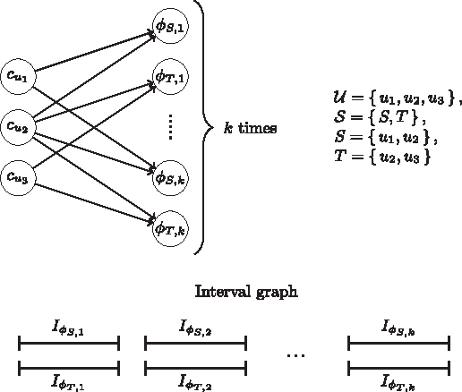
all with weight 1 (Fig. 4). This means that once we choose to open the facility φ_S_,i, we are essentially covering all of the elements u′ ∈ S, by assigning all of the clients \documentclass{aastex}\usepackage{amsbsy}\usepackage{amsfonts}\usepackage{amssymb}\usepackage{bm}\usepackage{mathrsfs}\usepackage{pifont}\usepackage{stmaryrd}\usepackage{textcomp}\usepackage{portland, xspace}\usepackage{amsmath, amsxtra}\pagestyle{empty}\DeclareMathSizes{10}{9}{7}{6}\begin{document} $${ {\cal C}}_{u^{ \prime}}$$ \end{document} to φ_S_,i.

FIG. 4.
An example of a reduction from the maximum coverage problem to the maximum facility location problem. In this instance, there are three elements (u₁, u₂, and u₃) and two subsets (S and T). Given an integer k, we create k intervals for each subset and create k cliques. In each clique, every pair of intervals overlaps. This means we can select at most k subsets.

We now argue that the value of the maximum facility location instance equals the value of the maximum coverage instance. Let Φ be the set of facilities opened and \documentclass{aastex}\usepackage{amsbsy}\usepackage{amsfonts}\usepackage{amssymb}\usepackage{bm}\usepackage{mathrsfs}\usepackage{pifont}\usepackage{stmaryrd}\usepackage{textcomp}\usepackage{portland, xspace}\usepackage{amsmath, amsxtra}\pagestyle{empty}\DeclareMathSizes{10}{9}{7}{6}\begin{document} $${ {\cal C}}_{ \Phi}$$ \end{document} be the corresponding subsets we choose from the collection \documentclass{aastex}\usepackage{amsbsy}\usepackage{amsfonts}\usepackage{amssymb}\usepackage{bm}\usepackage{mathrsfs}\usepackage{pifont}\usepackage{stmaryrd}\usepackage{textcomp}\usepackage{portland, xspace}\usepackage{amsmath, amsxtra}\pagestyle{empty}\DeclareMathSizes{10}{9}{7}{6}\begin{document} $${ {\cal S}}$$ \end{document} . Since we can pick at most one facility from each clique, and there are k of them, it follows that \documentclass{aastex}\usepackage{amsbsy}\usepackage{amsfonts}\usepackage{amssymb}\usepackage{bm}\usepackage{mathrsfs}\usepackage{pifont}\usepackage{stmaryrd}\usepackage{textcomp}\usepackage{portland, xspace}\usepackage{amsmath, amsxtra}\pagestyle{empty}\DeclareMathSizes{10}{9}{7}{6}\begin{document} $$\mid { {\cal C}}_ \Phi \mid \leq k$$ \end{document} .

In order to argue that the values are the same, we observe that by opening a facility φ_S_,i, we allow all of the clients connected to φ_S_,i to be assigned. Since all of the edge weights are 1, this corresponds to how many elements we cover if we select the subset S. The second observation is that the instance cannot benefit by opening the facility φ_S_,i and φ_S_{, j} for j≠i, as a client can only be assigned to a single open facility. This directly corresponds to covering no new elements.

Then from the discussion above and the inapproximability result (Feige, 1998; Khuller et al., 1999) for maximum coverage, we arrive at the theorem. ■

5. Experiments

While we believe that our general scheme can be useful in the analysis of various biological questions by Seq assays, in this proof of concept we focus on the detection of deletions in a donor genome with respect to a reference genome. We implemented the engineered independent rounding with alteration (Independent) and the dependent rounding algorithm (Dependent). Our implementation was done in Java 1.8, using Gurobi gur (2015) to solve the linear program. We also solve the integer program (IP) for benchmarking purposes.

To mimic the conflict resolution approach of VariationHunter (Hormozdiari et al., 2010) (see the section Related Work), we further implemented two simple greedy algorithms. The first method chooses a facility at each iteration that leads to the highest increase in value [according to the objective in Eq. (1)] that does not conflict with the current set (wGreedy). The second method picks the facility that covers the largest number of new clients (Greedy). Experiments were run on a quad-core Intel Core i7 processor running at 2.7 GHz with 16 GB of RAM. In the following, we evaluate the performance of our method on both simulated data and a real Illumina sequencing data set.

5.1. Simulated reads: Craig Venter

We use the benchmark data set designed in Marschall et al. (2012) for the evaluation of algorithms that reconstruct structural variants (SV) from NGS reads. In short, Craig Venter's genome is modeled by inserting annotated structural variants (Levy et al., 2007) into the reference genome. From the resulting two different alleles, 100 bp paired-end reads from fragments of mean length μ = 312 (σ = 15) were simulated using UCSC's SimSeq. All reads (30×) were aligned to reference genome hg 18 using BWA (Li and Durbin, 2009), allowing up to 25 alignments per read. The read alignments were provided in Marschall et al. (2012) as input to the proposed method CLEVER and all competing state-of-the-art SV discovery methods. The performance of the different tools in predicting insertions and deletions was measured in terms of recall = TP/(TP+FN) and precision = TP/(TP+FP), where a predicted deletion counts as true positive (TP) if it overlaps a true deletion and differs in length by no more than 100 bp (∼ mean distance between reads of same fragment). In this metric, CLEVER performed particularly well in the prediction of deletions of size 20–99 bp, compared to previous insert size-based approaches. The authors observed, however, a large fraction of false positive calls (30% in the 20–49 bp range) caused by misalignments and mapping ambiguities.

Here, we demonstrate the ability of our method to guide the selection of a core subset of deletions among many candidate predictions by resolving conflicts resulting from ambiguous mappings. More specifically, we compile CLEVER's output of statistically significant deletions into an instance of the maximum facility location problem. From the opened facilities we derive our final prediction of deletions in Venter's genome. Since we do not intend to provide a comprehensive method for the detection of structural variants, we refrain from comparing the overall performance to alternative SV discovery methods. On the contrary, our scheme can be applied to the set of candidate predictions computed by any soft clustering-based SV caller.

Table 1 shows recall and precision achieved by the different algorithms. In the defintion of TP we avoid a single deletion to be explained by several (different) predictions and a single prediction to explain multiple true deletions by computing a maximum cardinality matching between predicted deletions and true deletions. Each method was provided with all significant deletions called by CLEVER (Marschall et al., 2012) (CLEVER-cand). Analogously to the evaluation in Marschall et al. (2012), we consider deletions of size 20–49 (8,502 true del.), 50–99 (1,822 true del.), and 100–50,000 bases (2,996 true del.). Deletions of size less than 20 bases are difficult to discover by an insert-size-based scheme as implemented by CLEVER. CLEVER also offers a script to filter variants that are located too close to each other. We include the evaluation of this filtered set of predictions (CLEVER-filter).

Table 1.
Results on Simulated Craig Venter Data Set

Rec. 20–49* Rec. 50–99 Rec. 100–50 kb Recall Precision Runtime

CLEVER-cand 66.80 79.47 68.49 68.91 9.93 N/A

CLEVER-filter 46.26 64.38 66.76 53.35 51.06 <1

Independent 62.37 75.30 66.29 65.02 40.63 15.8

Dependent 63.10 75.96 66.32 65.59 40.49 4.5

IP 63.46 75.96 66.26 65.80 40.26 10.4

Greedy 63.02 75.14 66.42 65.44 41.47 1840.0

wGreedy 62.86 74.97 66.29 65.29 41.42 4095.0

Recall and precision achieved by the different algorithms when provided with the candidate predictions of CLEVER (Marschall et al., 2012) (CLEVER-cand) on the simulated Craig Venter data set. We report recall for deletions of different length in a-b bases (Rec. a-b) as well as overall recall and overall precision. The last column gives the total running time in minutes.

All methods are able to reduce the number of false postive calls made by CLEVER significantly, at only a small cost in recall. The very similar accuracy of the predictions obtained by the maximum facility location algorithms and the greedy algorithms is remarkable, since they are based on different mathematical models. While the latter seeks a minimal set of deletions (facilities) to explain all reads, the algorithms developed in this work rely exclusively on alignment scores and conflicts between deletions and do not impose any further assumptions. In contrast, the post-processing step optionally applied by CLEVER suffers from a significant loss in recall, in particular in the relevant range of 20–99 base-long deletions. Although this filtering scheme targets (a relaxed definition of) conflicts, it neglects ambiguous mappings of reads.

In terms of runtime performance, the most notable trend is that the greedy heuristics were two orders of magnitude slower than the LP-rounding heuristics, taking days rather than minutes to find a solution. This is because the greedy algorithms need to evaluate the objective function (1) many times, which can be expensive for large instances. Compare this to our solutions, which solve an LP and evaluate the objective function a few times. Surprisingly, the IP solver showed a performance comparable to our heuristics. This is probably due to the fact that the IP approach involves a single call to the highly optimized Gurobi software library written in C, while our implementation uses Java. Nevertheless, we expect our rounding algorithms to scale better on larger instances.

5.2. Illumina reads: NA12878

Real data pose unique challenges like PCR artefacts or chimeric reads to a computational analysis. We thus evaluate the performance of our method on publicly available Illumina sequencing data of the well-studied NA12878 individual (European Nucleotide Archive, ERA172924). In total, 101 bp reads were sequenced (50×) from the ends of fragments whose mean length μ was empirically estimated by CLEVER to be 320.89 bp (σ = 66.56).

We followed the same protocol as with the simulated benchmark. We cast statistically significant deletions predicted by CLEVER as our input facilities F. From facilities opened by our algorithm(s) we derive our final prediction of deletions in NA12878's genome. We measured recall and precision of deletion calling on chromosomes 1 through X with respect to two truth sets made available by Layer et al. (2014). The first truth set (1000G) contains 3,376 nonoverlapping deletions validated in NA12878 by the Mills et al. study (2011). The second truth set (long-read) comprises 4,095 predicted deletions that were validated by PacBio or Illumina Moleculo long-read sequencing data [for details see Layer et al. (2014)].

Since for this real data set not the complete set of true deletions is known, we applied the following precision correction to the output of all benchmarked methods. Predicted deletions \documentclass{aastex}\usepackage{amsbsy}\usepackage{amsfonts}\usepackage{amssymb}\usepackage{bm}\usepackage{mathrsfs}\usepackage{pifont}\usepackage{stmaryrd}\usepackage{textcomp}\usepackage{portland, xspace}\usepackage{amsmath, amsxtra}\pagestyle{empty}\DeclareMathSizes{10}{9}{7}{6}\begin{document} $${ {\cal D}}$$ \end{document} that do not match any true deletion and that are not supported by at least one read that in turn supports at least one true deletion through one of its alternative alignments do not count as false positive hits. By definition, there exists no mapping of the set of reads supporting one of the deletions in \documentclass{aastex}\usepackage{amsbsy}\usepackage{amsfonts}\usepackage{amssymb}\usepackage{bm}\usepackage{mathrsfs}\usepackage{pifont}\usepackage{stmaryrd}\usepackage{textcomp}\usepackage{portland, xspace}\usepackage{amsmath, amsxtra}\pagestyle{empty}\DeclareMathSizes{10}{9}{7}{6}\begin{document} $${ {\cal D}}$$ \end{document} that would contribute any true positive hit, potentially due to true deletions in NA12878's genome that are missing in our truth set. Thus there is no meaningful way of comparing the performance of postprocessing methods among predictions in \documentclass{aastex}\usepackage{amsbsy}\usepackage{amsfonts}\usepackage{amssymb}\usepackage{bm}\usepackage{mathrsfs}\usepackage{pifont}\usepackage{stmaryrd}\usepackage{textcomp}\usepackage{portland, xspace}\usepackage{amsmath, amsxtra}\pagestyle{empty}\DeclareMathSizes{10}{9}{7}{6}\begin{document} $${ {\cal D}}$$ \end{document} , and their inclusion would blur the results on the remaining predictions where the existence of an alternative assignment to a true deletion indicates a true false postive prediction.

The number of (validated) true deletions for NA128787 in the relevant ranges of 20–49 and 50–99 are with 47 and 156 for 1000G and with 101 and 522 for long-read relatively small and thus the precise recall values have to be considered with care. The overall trend, however, seems to agree with the results on the simulated data set (Table 2).

Table 2.
Results on Illumina Data Set for NA12878

Rec. 20–49 Rec. 50–99 Rec. 100–50 kb Rec. Precision Runtime

1000G (47,156,2989)

CLEVER-cand 5.4 35.2 65.8 63.5 8.8 N/A

CLEVER-filter 5.4 34.6 63.2 61.1 53.26 <1

IP 5.4 34.0 62.4 60.3 69.3 10.5

Dependent 5.4 34.0 62.3 60.1 69.03 3.1

Independent 5.4 34.0 62.3 60.2 69.11 7.0

Greedy 5.4 34.6 62.2 60.2 69.79 1737.5

wGreedy 5.4 34.6 62.4 60.3 69.99 4947.2

Long-read (101,522,3443)

CLEVER-cand 23.5 44.5 79.5 73.9 9.9 N/A

CLEVER-filter 20.0 37.0 72.4 66.8 71.0 <1

IP 18.8 38.4 72.6 67.1 78.9 10.5

Dependent 20.0 38.4 73.0 67.4 79.4 3.1

Independent 20.0 38.2 73.0 67.4 79.5 7.0

Greedy 20.0 37.8 72.6 67.1 80.1 1737.5

wGreedy 20.0 37.8 72.3 66.8 79.8 4947.2

Recall and precision with respect to truth sets 1000G and long-read achieved by the different algorithms when provided with the candidate predictions of CLEVER (Marschall et al., 2012) (CLEVER-cand) on the Illumina data set for NA12878. We report recall for deletions of different length in a-b bases (Rec. a-b) as well as overall recall and overall precision. The number of true deletions in the three different size ranges are shown in brackets for the two truth sets. The last column gives the total running time in minutes.

Again, with a rather modest loss in recall we are able to increase the precision with respect to truth sets 1000G and long-read from 8.8% to around 69%, and from 9.9% to around 79%, respectively. Similar to the results on the simulated data set, the approximate or optimal solutions our algorithms find for the maximum facility location formulation are similar in terms of recall and precision to the ones returned by the greedy heuristics. In contrast to the greedy approach, however, our algorithms compute these solutions in the order of minutes rather than days. Compared to the heuristic filtering strategy optionally applied by CLEVER we increase the precision with respect to truth sets 1000G and long-read by ∼30% and ∼11%, respectively.

6. Conclusion and Discussion

We presented a universal framework for resolving conflicting predictions from ambiguous read mappings and demonstrated, as proof of concept, its utility in reporting a final set of deletions given a large set of candidate deletions. Since our model formulates conflicts as overlaps of intervals but does not impose any further assumptions like parsimony, we expect it to be useful in a wide range of reference-based NGS data analysis.

For instance, the algorithm proposed in Eslami Rasekh et al. (2015) clusters clones (fosmids or bacterial artificial chromosomes, BACs) split by a (putative) inversion breakpoint to discover large inversions. The authors observed that a parsimony objective similar to the one applied in VariationHunter (and evaluated in our experiments) fails to properly resolve ambiguities among breakpoints located in highly repetitive regions. Furthermore, our model might be useful in identifying tumor-specific deletions from matched tumor/normal samples based on their conflict and ambiguous mappings (Wittler and Chauve, 2011) as well as in resolving intersecting quasi-cliques enumerated to cluster metagenomic sequences (Yang et al., 2013). In contrast to a more restrictive definition of candidates as single cliques in each connected component (Ratan et al., 2015), the ability to resolve conflicts allows a more sensitive prediction of candidates.

The key assumption of our model that determines the range of potential applications is that conflicts can be formulated as the overlap of genomic intervals. It captures many features of haploid and diploid organisms, except for rare overlapping events on different alleles, which require a specialized treatment (Wittler, 2013). Conflicts in a mixture of cancerous and healthy cells, however, are inadequately covered by simple interval overlaps (Wittler, 2013) and will require a generalization of our model. Also, features like the DNA methylation status naturally relate to individual bases rather than genomic intervals.

7. Appendix: A Missing Proofs

Proof (of Lemma 3). We focus on a fixed but arbitrary client u ∈C. Let us rename the facilities v₁,v₂,…,v_k so that w_uv1 ≤ w_uv2 ≤ … ≤ w_{uv_k}, and define \documentclass{aastex}\usepackage{amsbsy}\usepackage{amsfonts}\usepackage{amssymb}\usepackage{bm}\usepackage{mathrsfs}\usepackage{pifont}\usepackage{stmaryrd}\usepackage{textcomp}\usepackage{portland, xspace}\usepackage{amsmath, amsxtra}\pagestyle{empty}\DeclareMathSizes{10}{9}{7}{6}\begin{document} $$w_{uv_0} = 0$$ \end{document} . Finally, set w(u) = max _v ∈Rw_uv.

We aim to show that E[w(u)], the contribution of u to E[f (R)], is at least a constant times \documentclass{aastex}\usepackage{amsbsy}\usepackage{amsfonts}\usepackage{amssymb}\usepackage{bm}\usepackage{mathrsfs}\usepackage{pifont}\usepackage{stmaryrd}\usepackage{textcomp}\usepackage{portland, xspace}\usepackage{amsmath, amsxtra}\pagestyle{empty}\DeclareMathSizes{10}{9}{7}{6}\begin{document} $$\sum \nolimits_{v \in F} w_{uv} \ x_{uv}$$ \end{document} , the contribution of u to the value of (x, y).

Let \documentclass{aastex}\usepackage{amsbsy}\usepackage{amsfonts}\usepackage{amssymb}\usepackage{bm}\usepackage{mathrsfs}\usepackage{pifont}\usepackage{stmaryrd}\usepackage{textcomp}\usepackage{portland, xspace}\usepackage{amsmath, amsxtra}\pagestyle{empty}\DeclareMathSizes{10}{9}{7}{6}\begin{document} $${ \hat {Y}}_v$$ \end{document} be an indicator variable that is 1 if v ∈R and 0 otherwise, then \documentclass{aastex}\usepackage{amsbsy}\usepackage{amsfonts}\usepackage{amssymb}\usepackage{bm}\usepackage{mathrsfs}\usepackage{pifont}\usepackage{stmaryrd}\usepackage{textcomp}\usepackage{portland, xspace}\usepackage{amsmath, amsxtra}\pagestyle{empty}\DeclareMathSizes{10}{9}{7}{6}\begin{document} \begin{align} { \rm Pr } [ w ( u ) < w_ { uv_i } ] & = { \rm Pr } \left[ \bigwedge_ { j = i } ^k \hat Y_ { v_j } = 0 \right] \\ & = \prod_ { j = i } ^k { \rm Pr } [ \hat { Y } _ { v_j } = 0 ] = \prod_ { j = i } ^k ( 1 - \alpha y_ { v_j } ) \\ & \leq \left( 1 - \frac { \alpha \sum \nolimits_ { j = i } ^k x_ { uv_j } } { k - i + 1 } \right) ^ { k - i + 1 } , \end{align} \end{document}

where the last inequality follows from the arithmetic-mean geometric-mean inequality and the feasibility of (x, y).

Let \documentclass{aastex}\usepackage{amsbsy}\usepackage{amsfonts}\usepackage{amssymb}\usepackage{bm}\usepackage{mathrsfs}\usepackage{pifont}\usepackage{stmaryrd}\usepackage{textcomp}\usepackage{portland, xspace}\usepackage{amsmath, amsxtra}\pagestyle{empty}\DeclareMathSizes{10}{9}{7}{6}\begin{document} $$\tilde{x} = \sum \nolimits_{j = i}^k x_{uv_j}$$ \end{document} and r = k−i + 1. We observe that the function \documentclass{aastex}\usepackage{amsbsy}\usepackage{amsfonts}\usepackage{amssymb}\usepackage{bm}\usepackage{mathrsfs}\usepackage{pifont}\usepackage{stmaryrd}\usepackage{textcomp}\usepackage{portland, xspace}\usepackage{amsmath, amsxtra}\pagestyle{empty}\DeclareMathSizes{10}{9}{7}{6}\begin{document} $$a ( \tilde { x } ) = 1 - \left( 1 - \frac { \alpha \tilde { x } } { r } \right) ^ { r } $$ \end{document} is concave on the interval \documentclass{aastex}\usepackage{amsbsy}\usepackage{amsfonts}\usepackage{amssymb}\usepackage{bm}\usepackage{mathrsfs}\usepackage{pifont}\usepackage{stmaryrd}\usepackage{textcomp}\usepackage{portland, xspace}\usepackage{amsmath, amsxtra}\pagestyle{empty}\DeclareMathSizes{10}{9}{7}{6}\begin{document} $$\tilde{x} \in [ 0 , 1 ]$$ \end{document} , and thus can be lowerbounded by the linear function \documentclass{aastex}\usepackage{amsbsy}\usepackage{amsfonts}\usepackage{amssymb}\usepackage{bm}\usepackage{mathrsfs}\usepackage{pifont}\usepackage{stmaryrd}\usepackage{textcomp}\usepackage{portland, xspace}\usepackage{amsmath, amsxtra}\pagestyle{empty}\DeclareMathSizes{10}{9}{7}{6}\begin{document} $$b ( \tilde { x } ) = \left[ 1 - \left( 1 - \frac { \alpha } { r } \right) ^ { r } \right] \tilde { x } $$ \end{document} . This is because a(0) = b(0) and a(1) = b(1). Therefore, \documentclass{aastex}\usepackage{amsbsy}\usepackage{amsfonts}\usepackage{amssymb}\usepackage{bm}\usepackage{mathrsfs}\usepackage{pifont}\usepackage{stmaryrd}\usepackage{textcomp}\usepackage{portland, xspace}\usepackage{amsmath, amsxtra}\pagestyle{empty}\DeclareMathSizes{10}{9}{7}{6}\begin{document} \begin{align} { \rm Pr } [ w ( u ) \ge w_ { uv_i } ] & = 1 - { \rm Pr } [ w ( u ) < w_ { uv_i } ] \\ & \ge 1 - \left( 1 - \frac { \alpha \sum \nolimits_ { j = i } ^k x_ { uv_j } } { k - i + 1 } \right) ^ { k - i + 1 } \\ & \ge \left[ 1 - \left( 1 - \frac { \alpha } { k - i + 1 } \right) ^ { k - i + 1 } \right] \mathop \sum \limits_ { j = i } ^k x_ { uv_j } \\ & \ge ( 1 - e^ { - \alpha } ) \mathop \sum \limits_ { j = i } ^k x_ { uv_j } . \end{align} \end{document}

We now express E[w(u)] in terms of Pr[w(u) ≥ w_{uv_i}] \documentclass{aastex}\usepackage{amsbsy}\usepackage{amsfonts}\usepackage{amssymb}\usepackage{bm}\usepackage{mathrsfs}\usepackage{pifont}\usepackage{stmaryrd}\usepackage{textcomp}\usepackage{portland, xspace}\usepackage{amsmath, amsxtra}\pagestyle{empty}\DeclareMathSizes{10}{9}{7}{6}\begin{document} \begin{align}{ \rm E} [ w ( u ) ] & = \mathop \sum \limits_{j = 1}^k w_{uv_j} { \rm Pr} [ w ( u ) = w_{uv_j} ] \\ & = \mathop \sum \limits_{j = 1}^k \left( \mathop \sum \limits_{i = 1}^j w_{uv_i} - w_{uv_{i - 1}} \right) { \rm Pr} [ w ( u ) = w_{uv_j} ] \\ & = \mathop \sum \limits_{i = 1}^k \mathop \sum \limits_{j = i}^k ( w_{uv_i} - w_{uv_{i - 1}} ) { \rm Pr} [ w ( u ) = w_{uv_j} ] \\ & = \mathop \sum \limits_{i = 1}^k ( w_{uv_i} - w_{uv_{i - 1}} ) { \rm Pr} [ w ( u ) \ge w_{uv_i} ] \end{align} \end{document}

Now we can use our bound on Pr[w(u) ≥ w_{uv_i}] to lowerbound the expected value of w(u) \documentclass{aastex}\usepackage{amsbsy}\usepackage{amsfonts}\usepackage{amssymb}\usepackage{bm}\usepackage{mathrsfs}\usepackage{pifont}\usepackage{stmaryrd}\usepackage{textcomp}\usepackage{portland, xspace}\usepackage{amsmath, amsxtra}\pagestyle{empty}\DeclareMathSizes{10}{9}{7}{6}\begin{document} \begin{align}{ \rm E} [ w ( u ) ] & = \mathop \sum \limits_{i = 1}^k ( w_{uv_i} - w_{uv_{i - 1}} ) { \rm Pr} [ w ( u ) \ge w_{uv_i} ] \\ & \ge ( 1 - e^{ - \alpha} ) \mathop \sum \limits_{i = 1}^k ( w_{uv_i} - w_{uv_{i - 1}} ) \mathop \sum \limits_{j = i}^k x_{uv_j} \\ & = ( 1 - e^{ - \alpha} ) \left( \mathop \sum \limits_{i = 1}^k \mathop \sum \limits_{j = i}^k w_{uv_j}x_{uv_j} - \mathop \sum \limits_{i = 1}^k \mathop \sum \limits_{j = i}^k w_{uv_{i - 1}} x_{uv_j} \right) \\ & = ( 1 - e^{ - \alpha} ) \mathop \sum \limits_{j = 1}^k x_{uv_j} \mathop \sum \limits_{i = 1}^j ( w_{uv_i} - w_{uv_{i - 1}} ) = ( 1 - e^{ - \alpha} ) \mathop \sum \limits_{j = 1}^k x_{uv_j} w_{uv_j}.\end{align} \end{document}

Finally, by linearity of expectation, we have \documentclass{aastex}\usepackage{amsbsy}\usepackage{amsfonts}\usepackage{amssymb}\usepackage{bm}\usepackage{mathrsfs}\usepackage{pifont}\usepackage{stmaryrd}\usepackage{textcomp}\usepackage{portland, xspace}\usepackage{amsmath, amsxtra}\pagestyle{empty}\DeclareMathSizes{10}{9}{7}{6}\begin{document} \begin{align}{ \rm E} [ f ( R ) ] = \mathop \sum \limits_{u \in C} { \rm E} [ w ( u ) ] \ge ( 1 - e^{ - \alpha} ) \mathop \sum \limits_{u \in C , v \in F} x_{uv} w_{uv} ,\end{align} \end{document}

which is precisely what we needed to prove. ■

	Rec. 20–49	Rec. 50–99	Rec. 100–50 kb	Recall	Precision	Runtime
CLEVER-cand	66.80	79.47	68.49	68.91	9.93	N/A
CLEVER-filter	46.26	64.38	66.76	53.35	51.06	<1
Independent	62.37	75.30	66.29	65.02	40.63	15.8
Dependent	63.10	75.96	66.32	65.59	40.49	4.5
IP	63.46	75.96	66.26	65.80	40.26	10.4
Greedy	63.02	75.14	66.42	65.44	41.47	1840.0
wGreedy	62.86	74.97	66.29	65.29	41.42	4095.0

	Rec. 20–49	Rec. 50–99	Rec. 100–50 kb	Rec.	Precision	Runtime
1000G (47,156,2989)
CLEVER-cand	5.4	35.2	65.8	63.5	8.8	N/A
CLEVER-filter	5.4	34.6	63.2	61.1	53.26	<1
IP	5.4	34.0	62.4	60.3	69.3	10.5
Dependent	5.4	34.0	62.3	60.1	69.03	3.1
Independent	5.4	34.0	62.3	60.2	69.11	7.0
Greedy	5.4	34.6	62.2	60.2	69.79	1737.5
wGreedy	5.4	34.6	62.4	60.3	69.99	4947.2
Long-read (101,522,3443)
CLEVER-cand	23.5	44.5	79.5	73.9	9.9	N/A
CLEVER-filter	20.0	37.0	72.4	66.8	71.0	<1
IP	18.8	38.4	72.6	67.1	78.9	10.5
Dependent	20.0	38.4	73.0	67.4	79.4	3.1
Independent	20.0	38.2	73.0	67.4	79.5	7.0
Greedy	20.0	37.8	72.6	67.1	80.1	1737.5
wGreedy	20.0	37.8	72.3	66.8	79.8	4947.2

Footnotes

Acknowledgments

We thank Tobias Marshall for valuable support in the interpretation of CLEVER's output.

Author Disclosure Statement

The authors declare that no competing financial interests exist.

References

Cooper

G.M.

, Nickerson

D.A.

, and Eichler

E.E.

2007. Mutational and selective effects on copy-number variants in the human genome. Nat. Genet., 39, S22–S29.

Feige

1998. A threshold of ln n for approximating set cover. J. ACM, 45, 634–652.

Feldman

2013. Maximization problems with submodular objective functions [Ph.D. thesis]. Israel Institute of Technology, Israel.

Gandhi

, Khuller

, Parthasarathy

, et al. 2006. Dependent rounding and its applications to approximation algorithms. J. ACM, 53, 324–360.

Gurobi. An easier way to make better decisions. 2015. Available at: www.gurobi.com. Accessed May 15, 2015.

Hach

, Hormozdiari

, Alkan

, et al. 2010. mrsFAST: a cache-oblivious algorithm for short-read mapping. Nat. Methods, 7, 576–577.

Hormozdiari

, Alkan

, Eichler

E.E.

, et al. 2009. Combinatorial algorithms for structural variation detection in high-throughput sequenced genomes. Genome Res. 19, 1270–1278.

Hormozdiari

, Hajirasouliha

, Dao

, et al. 2010. Next-generation variationhunter: combinatorial algorithms for transposon insertion discovery. Bioinformatics, 26, i350–i357.

Hormozdiari

, Hajirasouliha

, McPherson

, et al. 2011. Simultaneous structural variation discovery among multiple paired-end sequenced genomes. Genome Res. 21, 2203–2212.

10.

Khuller

, Moss

, and Naor

J.S.

1999. The budgeted maximum coverage problem. Inform. Process. Lett., 70, 39–45.

11.

Kim

P.M.

, Lam

H.Y.

, Urban

A.E.

, et al. 2008. Analysis of copy number variants and segmental duplications in the human genome: evidence for a change in the process of formation in recent evolutionary history. Genome Res. 18, 1865–1874.

12.

Layer

, Chiang

, Quinlan

, et al. 2014. LUMPY: a probabilistic framework for structural variant discovery. Genome Biol. 15, R84.

13.

Lee

, Cheran

, and Brudno

2008. A robust framework for detecting structural variations in a genome. Bioinformatics, 24, i59–i67.

14.

Levy

, Sutton

, Ng

P.C.

, et al. 2007. The diploid genome sequence of an individual human. PLoS Biol. 5, e254.

15.

, and Durbin

2009. Fast and accurate short read alignment with burrows? Wheeler transform. Bioinformatics, 25, 1754–1760.

16.

Marschall

, Costa

I.G.

, Canzar

, et al. 2012. Clever: clique-enumerating variant finder. Bioinformatics, 28, 2875–2882.

17.

Medvedev

, Stanciu

, and Brudno

2009. Computational methods for discovering structural variation with next-generation sequencing. Nat. Methods, 6, S13–S20.

18.

Mills

R.E.

, Walter

, Stewart

, et al. 2011. Mapping copy number variation by population-scale genome sequencing. Nature, 470, 59–65.

19.

Pleasance

E.D.

, Cheetham

R.K.

, Stephens

P.J.

, et al. 2009. A comprehensive catalogue of somatic mutations from a human cancer genome. Nature, 463, 191–196.

20.

Rasekh

M.E.

, Chiatante

, Miroballo

, et al. 2015. Discovery of large genomic inversions using pooled clone sequencing. bioRxiv. DOI: https://dx-doi-org.web.bisu.edu.cn/10.1101/015156

21.

Ratan

, Olson

T.L.

, Loughran

T.P.

Jr. , et al. 2015. Identification of indels in next-generation sequencing data. BMC Bioinform. 16, 42.

22.

Vondrák

, Chekuri

, and Zenklusen

2011. Submodular function maximization via the multilinear relaxation and contention resolution schemes, 783–792. In Proceedings of the Forty-Third Annual ACM Symposium on Theory of Computing. ACM, New York, NY.

23.

Wittler

2013. Unraveling overlapping deletions by agglomerative clustering. BMC Genomics, 14, S12.

24.

Wittler

, and Chauve

2011. Consistency-based detection of potential tumor-specific deletions in matched normal/tumor genomes. BMC Bioinform. 12, S21.

25.

Yang

, Zola

, and Aluru

2013. Large-scale metagenomic sequence clustering on map-reduce clusters. J. Bioinform. Comput. Biol. 11, 1340001.