Deep Feature Selection: Theory and Application to Identify Enhancers and Promoters

Abstract

Sparse linear models approximate target variable(s) by a sparse linear combination of input variables. Since they are simple, fast, and able to select features, they are widely used in classification and regression. Essentially they are shallow feed-forward neural networks that have three limitations: (1) incompatibility to model nonlinearity of features, (2) inability to learn high-level features, and (3) unnatural extensions to select features in a multiclass case. Deep neural networks are models structured by multiple hidden layers with nonlinear activation functions. Compared with linear models, they have two distinctive strengths: the capability to (1) model complex systems with nonlinear structures and (2) learn high-level representation of features. Deep learning has been applied in many large and complex systems where deep models significantly outperform shallow ones. However, feature selection at the input level, which is very helpful to understand the nature of a complex system, is still not well studied. In genome research, the cis-regulatory elements in noncoding DNA sequences play a key role in the expression of genes. Since the activity of regulatory elements involves highly interactive factors, a deep tool is strongly needed to discover informative features. In order to address the above limitations of shallow and deep models for selecting features of a complex system, we propose a deep feature selection (DFS) model that (1) takes advantages of deep structures to model nonlinearity and (2) conveniently selects a subset of features right at the input level for multiclass data. Simulation experiments convince us that this model is able to correctly identify both linear and nonlinear features. We applied this model to the identification of active enhancers and promoters by integrating multiple sources of genomic information. Results show that our model outperforms elastic net in terms of size of discriminative feature subset and classification accuracy.

1. Introduction

Sparse regularized linear models are widely used in machine learning and bioinformatics for classification and regression. These models are shallow feed-forward neural networks that approximate the response variable by a sparse superposition of input variables (or features), that is, y ≈ f ( x ) = x ^T w + b. From a maximum a posteriori (MAP) estimation (or regularization) perspective, its optimization can be generally formulated to min_{w
,b} f ( w , b) = l( w , b) + λr( w ), where l( w , b) is a loss function corresponding to the negative log-likelihood of data, and r( w ) is a sparse regularization term corresponding to the prior of model parameter. Typical loss functions include 0-1 loss, hinge loss, logistic loss (for classification), squared loss (for both classification and regression), ɛ-sensitive loss (for regression), etc. A regularization term aims to reduce model complexity, thus avoids overfitting. Also, a sparse regularization can help to select features by taking features with nonzero weights in w . Commonly used sparse regularization terms include l₁-norm (LASSO) (Tibshirani, 1996), non-negativity (Li and Ngom, 2013), and SCAD (Bradley and Mangasarian, 1998). LASSO and its variant, elastic net (Zou and Hastie, 2005) [as formulated in Eq. (1)], are among the most popularly used techniques. \documentclass{aastex}\usepackage{amsbsy}\usepackage{amsfonts}\usepackage{amssymb}\usepackage{bm}\usepackage{mathrsfs}\usepackage{pifont}\usepackage{stmaryrd}\usepackage{textcomp}\usepackage{portland, xspace}\usepackage{amsmath, amsxtra}\pagestyle{empty}\DeclareMathSizes{10}{9}{7}{6}\begin{document} \begin{align*}\begin{cases} { \rm LASSO } : \quad \quad r ( \textbf { \textit { w } } ) = \parallel \textbf { \textit { w } } \parallel_1 \\ { \rm elastic \ net } : \quad r ( \textbf { \textit { w } } ) = \frac { 1 - \alpha } { 2 } \parallel \textbf { \textit { w } } \parallel_2^2 + \alpha \parallel \textbf { \textit { w } } \parallel_1 \end{cases} \tag { 1 } \end{align*} \end{document}

LASSO is a special case of elastic net by setting α = 1.

The popularity of sparse linear models is due to the following reasons. First, their concept is easy to understand. Second, variables can be selected. Third, the learning of model parameter θ is often convex in the parameter landscape, thus many fast implementations are available. However, linear models have three main limitations. (1) Nonlinear correlation among variables cannot be considered (except by handcrafted features or a kernel extension). (2) High-level representation of features can not be learned due to the shallow structure. (3) There does not exist a “natural” way to extend a two-class linear model to multiclass case in classification and feature selection. Two common multiclass extensions are one-versus-one and one-versus-rest. The corresponding feature selection is accomplished by taking the union of results generated by two-class linear models. For instance, given C classes, softmax regression (a one-versus-rest multiclass extension of logistic regression, see Fig. 1A) with LASSO will produce C subsets of class-specific features. These subsets are then pooled as the final result. Since the final subset of features depends on one specific strategy of multi-class extension, different strategies may yield different results.

FIG. 1.

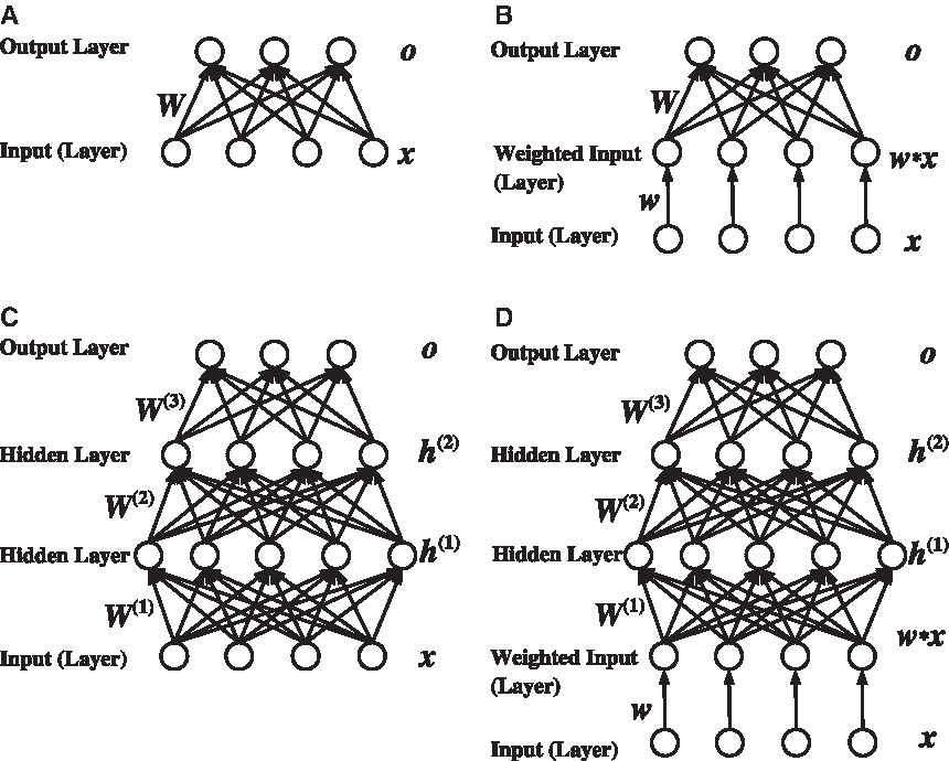
A structural comparison of our deep feature selection (DFS) models and previous ones. (A) Elastic net. (B) Shallow DFS. (C) Multilayer perceptron. (D) Deep DFS.

Through piling up hidden layers, deep neural networks are able to model nonlinearity of features. Figure 1C is an example of such a deep model called multilayer perceptrons (MLP), which is a deep feed-forward neural network. The techniques of learning deep models and their inferences fall into an active research frontier—deep learning (Hinton et al., 2006), which has four attractive strengths for applying it in complex intelligent systems: First, deep models often dramatically increase prediction accuracy. Second, they can model processes of complex systems. Third, they can generate structured high-level representations of features that can help the interpretation of data. Fourth, (convolutional) deep learning models are robust to temporal or spatial variation. But the learning of such models are usually nonconvex in optimization, and the back-propagation algorithm (a first-order method) does not perform well on deeper structures. The optimization strategy using greedy layer-wise unsupervised pretraining and finetuning, proposed in Hinton et al. (2006), is considered as a breakthrough. While high-level feature extraction and representation have been intensively studied in the surge of deep learning research (Bengio et al., 2013), feature selection at the input level is still not well studied. However, in bioinformatics and other studies on complex systems, selecting key input features are crucial to understanding the mechanisms of the systems. Thus, existing models mentioned above do not meet this need. In our current bioinformatics research, we are committed to devising a deep learning model for the identification and understanding of cis-regulatory elements in the human genome.

Genome researchers have discovered that noncoding DNA sequences (previously viewed as junk DNA) are composed of many regulatory elements (The ENCODE Project Consortium, 2012). These elements (including enhancers and promoters) precisely control the expression level of genes. Promoters are cis-acting DNA sequences that switch on or off the expression of genes, while enhancers are generally cis-acting DNA sequences that tune the expression level of genes (Shlyueva et al., 2014). A promoter resides close to its target gene, while an enhancer is distal to its target gene(s), making it difficult to identify. The identification of active enhancers and promoters in a genome is of key importance, as it can help to elucidate the regulatory mechanism in the genome and interpret disease-causing variants within cis-regulatory elements. However, since regulatory landscapes of DNA are quite different among cell types, and regulatory events are precisely and dynamically controlled by multiple factors, including epigenetic marks, transcription factors, microRNAs, and their interactions, it is a difficult task to identify active enhancers and promoters in a given cell type. The emergence of both deep sequencing and deep computing techniques casts light on this problem.

In order to select key input features for identifying and understanding regulatory events, we propose a deep feature selection model that enables variable selection for deep neural networks. In this model, a sparse one-to-one layer, where each input feature is weighted, is added between the input and the first hidden layer, giving two advantages: (1) a single subset of features for multiple classes (multiple output nodes) can be conveniently selected, which addresses the challenge of multiclass extension of linear models; and (2) through selecting features at the input level of the deep structure, we are able to identify informative features that have nonlinear behaviors.

2. Method

2.1. Deep feature selection

We focus our research on feature selection for multiclass data using deep neural networks. We propose a deep feature selection (DFS) model that can select features at the input level of a deep network. An example of such a model is illustrated in Figure 1D. Our main idea is to add a sparse one-to-one linear layer between the input layer and the first hidden layer of an MLP. In this one-to-one layer, the input feature x_i only connects to the i-th node with linear activation function. Thus, the output of the one-to-one layer becomes w * x , where * is element-wise multiplication. In order to select input features, w has to be sparse, and only the features corresponding to nonzero weights are selected. Although, we can resort to any sparse regularization term on w . In our current study, we use elastic net \documentclass{aastex}\usepackage{amsbsy}\usepackage{amsfonts}\usepackage{amssymb}\usepackage{bm}\usepackage{mathrsfs}\usepackage{pifont}\usepackage{stmaryrd}\usepackage{textcomp}\usepackage{portland, xspace}\usepackage{amsmath, amsxtra}\pagestyle{empty}\DeclareMathSizes{10}{9}{7}{6}\begin{document} $$\lambda_1 \left( \frac { 1 - \lambda_2 } { 2 } \parallel \textbf { \textit { w } } \parallel_2^2 + \lambda_2 \parallel \textbf { \textit { w } } \parallel_1 \right)$$ \end{document} (Zou and Hastie, 2005). Such a DFS model can be called deep elastic net. As in regular MLP, the activation function in the hidden layers of DFS is also nonlinear [e.g., sigmoid, tangent, or rectified linear unit (ReLU) (Nair and Hinton, 2010)]. The output layer is a softmax layer, where the output of unit i is defined as \documentclass{aastex}\usepackage{amsbsy}\usepackage{amsfonts}\usepackage{amssymb}\usepackage{bm}\usepackage{mathrsfs}\usepackage{pifont}\usepackage{stmaryrd}\usepackage{textcomp}\usepackage{portland, xspace}\usepackage{amsmath, amsxtra}\pagestyle{empty}\DeclareMathSizes{10}{9}{7}{6}\begin{document} \begin{align*}p ( y = i \mid \textbf { \textit { x } } ) = \frac { e^ { - \textbf { \textit { w } } _i^ { ( K + 1 ) ^ { \rm T } } \textbf { \textit { h } } ( K ) } } { \sum \nolimits_ { { c } = 1 } ^C e^ { - \textbf { \textit { w } } _ { \cal C } ^ { ( K + 1 ) ^ { \rm T } } } \textbf { \textit { h } } ^ { ( K ) } } , \tag { 2 } \end{align*} \end{document}

where \documentclass{aastex}\usepackage{amsbsy}\usepackage{amsfonts}\usepackage{amssymb}\usepackage{bm}\usepackage{mathrsfs}\usepackage{pifont}\usepackage{stmaryrd}\usepackage{textcomp}\usepackage{portland, xspace}\usepackage{amsmath, amsxtra}\pagestyle{empty}\DeclareMathSizes{10}{9}{7}{6}\begin{document} $$\textbf{\textit{w}}_i^{ ( K + 1 ) }$$ \end{document} is the i-th column of weight matrix \documentclass{aastex}\usepackage{amsbsy}\usepackage{amsfonts}\usepackage{amssymb}\usepackage{bm}\usepackage{mathrsfs}\usepackage{pifont}\usepackage{stmaryrd}\usepackage{textcomp}\usepackage{portland, xspace}\usepackage{amsmath, amsxtra}\pagestyle{empty}\DeclareMathSizes{10}{9}{7}{6}\begin{document} $$\textbf{\textit{W}}^{ ( K + 1 ) }$$ \end{document} from the last hidden layer (that is the K-th hidden layer) to the softmax layer. Our DFS model has at least two distinctive advantages. First, given a parameter setting, it always selects a single subset of features for multiclass problems. It overcomes the limitation of linear models for multiclass data, making feature selection more convenient. Second, by using a deep nonlinear structure, it can automatically identify nonlinear features, which is superior over shallow linear models.

2.2. Learning model parameter

Suppose there are K hidden layers in a DFS model. Its model parameter can be denoted by \documentclass{aastex}\usepackage{amsbsy}\usepackage{amsfonts}\usepackage{amssymb}\usepackage{bm}\usepackage{mathrsfs}\usepackage{pifont}\usepackage{stmaryrd}\usepackage{textcomp}\usepackage{portland, xspace}\usepackage{amsmath, amsxtra}\pagestyle{empty}\DeclareMathSizes{10}{9}{7}{6}\begin{document} $${ \boldsymbol{\theta}} = \{ \textbf{\textit{w}} , \textbf{\textit{W}}^{ ( 1 ) } , \textbf{\textit{b}}^{ ( 1 ) } , \cdots , \textbf{\textit{W}}^{ ( K + 1 ) } , \textbf{\textit{b}}^{ ( K + 1 ) } \} $$ \end{document} , where W ^(k) is the weight matrix connecting the k − 1-th layer to the k-th layer, and b ^(k) is the corresponding biases in the k-th layer. The size of W ^(k) is n_{k – 1} × n_k, where n_k is the number of units in the k-th layer. In order to learn the model parameter, we minimize the objective function below, \documentclass{aastex}\usepackage{amsbsy}\usepackage{amsfonts}\usepackage{amssymb}\usepackage{bm}\usepackage{mathrsfs}\usepackage{pifont}\usepackage{stmaryrd}\usepackage{textcomp}\usepackage{portland, xspace}\usepackage{amsmath, amsxtra}\pagestyle{empty}\DeclareMathSizes{10}{9}{7}{6}\begin{document} \begin{align*} \begin{split} \min_ { \boldsymbol{\theta} } \ f ( { \boldsymbol{\theta} } ) = & l ( { \boldsymbol{\theta} } ) + \lambda_1 \left( \frac { 1 - \lambda_2 } { 2 } \parallel \textbf { \textit { w } } \parallel_2^2 + \lambda_2 \parallel \textbf { \textit { w } } \parallel_1 \right) + \alpha_1 \left( \frac { 1 - \alpha_2 } { 2 } \mathop \sum \limits_ { k = 1 } ^ { K + 1 } \parallel \textbf { \textit { W } } ^ { ( k ) } \parallel_F^2 + \alpha_2 \mathop \sum \limits_ { k = 1 } ^ { K + 1 } \parallel \textbf { \textit { W } } ^ { ( k ) } \parallel_1 \right) , \end{split} \tag { 3 } \end{align*} \end{document}

which is explained as follows.

1. l( θ ) is the log-likelihood of data. From Equation (2), recall that the top layer of our model is a softmax regression model with a multinoulli distribution for the probability of targets: \documentclass{aastex}\usepackage{amsbsy}\usepackage{amsfonts}\usepackage{amssymb}\usepackage{bm}\usepackage{mathrsfs}\usepackage{pifont}\usepackage{stmaryrd}\usepackage{textcomp}\usepackage{portland, xspace}\usepackage{amsmath, amsxtra}\pagestyle{empty}\DeclareMathSizes{10}{9}{7}{6}\begin{document} \begin{align*} \begin{split} h_ { \theta } ( \textbf { \textit { h } } ^ { ( K ) } , { \boldsymbol{\theta}} ) & = \left[ \begin{matrix} p ( y = 1 \mid \textbf { \textit { h } } ^ { ( K ) } , {\boldsymbol{\theta}} ) \\ \vdots \\ p ( y = C \mid \textbf { \textit { h } } ^ { ( K ) } , { \boldsymbol{\theta} } ) \end{matrix} \right] \\ & = \frac { 1 } { \sum \nolimits_ { { c } = 1 } ^C e^ { - \textbf { \textit { w } } _ { \cal C } ^ { ( K + 1 ) ^ { \rm T } } \textbf { \textit { h } } ^ { ( k ) } - b_ { \cal C } ^ { ( K + 1 ) } } } \left[ \begin{matrix} e^ { - \textbf { \textit { w } } _1^ { ( K + 1 ) ^ { \rm T } } } \textbf { \textit { h } } ^ { ( K ) } - b_1^ { ( K + 1 ) } \\ \vdots \\ e^ { - \textbf { \textit { w } } _C^ { ( K + 1 ) ^ { \rm T } } } \textbf { \textit { h } } ^ { ( K ) } - b_C^ { ( K + 1 ) } \end{matrix} \right]. \end{split} \tag{4} \end{align*} \end{document} Therefore, l( θ ) in Equation (3) is \documentclass{aastex}\usepackage{amsbsy}\usepackage{amsfonts}\usepackage{amssymb}\usepackage{bm}\usepackage{mathrsfs}\usepackage{pifont}\usepackage{stmaryrd}\usepackage{textcomp}\usepackage{portland, xspace}\usepackage{amsmath, amsxtra}\pagestyle{empty}\DeclareMathSizes{10}{9}{7}{6}\begin{document} \begin{align*} \begin{split} l ( { \boldsymbol{\theta}} ) & = - \mathop \sum \limits_ { i = 1 } ^N \log p ( y_i \mid \textbf { \textit { h } } _i^ { ( K ) } ) \\ & = - \mathop \sum \limits_ { i = 1 } ^N \log \frac { e^ { - \textbf { \textit { w } } _ { y_i } ^ { ( K + 1 ) ^ { \rm T } } \textbf { \textit { h } } _i^ { ( K ) } - b_ { y_i } ^ { ( K + 1 ) } } } { \sum \nolimits_ { { c } = 1 } ^C e^ { - \textbf { \textit { w } } _ { { \cal C } } ^ { ( K + 1 ) ^ { \rm T } } } \textbf { \textit { h } } _i^ { ( K ) } - b_ { c } ^ { ( K + 1 ) } } \\ & = \mathop \sum \limits_ { i = 1 } ^N \left( \textbf { \textit { w } } _ { y_i } ^ { ( K + 1 ) ^ { \rm T } } \textbf { \textit { h } } _i^ { ( K ) } + b_ { y_i } ^ { ( K + 1 ) } + \log \mathop \sum \limits_ { { c } = 1 } ^C e^ { - \textbf { \textit { w } } _ { \cal C } ^ { ( K + 1 ) ^ { \rm T } } \textbf { \textit { h } } _i^ { ( K ) } - b_ { \cal C } ^ { ( K + 1 ) } } \right) , \end{split} \tag{5} \end{align*} \end{document}

2. Regularization term \documentclass{aastex}\usepackage{amsbsy}\usepackage{amsfonts}\usepackage{amssymb}\usepackage{bm}\usepackage{mathrsfs}\usepackage{pifont}\usepackage{stmaryrd}\usepackage{textcomp}\usepackage{portland, xspace}\usepackage{amsmath, amsxtra}\pagestyle{empty}\DeclareMathSizes{10}{9}{7}{6}\begin{document} $$\lambda_1 \left( \frac { 1 - \lambda_2 } { 2 } \parallel \textbf { \textit { w } } \parallel_2^2 + \lambda_2 \parallel \textbf { \textit { w } } \parallel_1 \right)$$ \end{document} is an elastic-net-like term, where user-specified parameter λ₂∈[0, 1] controls the trade-off between smoothness and sparsity of w . We note that ∥ w ∥₁ can be further generalized to \documentclass{aastex}\usepackage{amsbsy}\usepackage{amsfonts}\usepackage{amssymb}\usepackage{bm}\usepackage{mathrsfs}\usepackage{pifont}\usepackage{stmaryrd}\usepackage{textcomp}\usepackage{portland, xspace}\usepackage{amsmath, amsxtra}\pagestyle{empty}\DeclareMathSizes{10}{9}{7}{6}\begin{document} $$( 1 - \lambda_3 ) \parallel \textbf{\textit{w}} \parallel_{ +} + \lambda_3 \parallel \textbf{\textit{w}} \parallel_{ -}$$ \end{document} , where \documentclass{aastex}\usepackage{amsbsy}\usepackage{amsfonts}\usepackage{amssymb}\usepackage{bm}\usepackage{mathrsfs}\usepackage{pifont}\usepackage{stmaryrd}\usepackage{textcomp}\usepackage{portland, xspace}\usepackage{amsmath, amsxtra}\pagestyle{empty}\DeclareMathSizes{10}{9}{7}{6}\begin{document} $$\parallel \textbf{\textit{w}} \parallel_{ -} = \sum \nolimits_{i - 1}^M \mid w \mid_{ -} = \sum \nolimits_{i = 1}^M$$ \end{document} max(0, −w_i) is a hinge loss function that only penalizes negative values, and \documentclass{aastex}\usepackage{amsbsy}\usepackage{amsfonts}\usepackage{amssymb}\usepackage{bm}\usepackage{mathrsfs}\usepackage{pifont}\usepackage{stmaryrd}\usepackage{textcomp}\usepackage{portland, xspace}\usepackage{amsmath, amsxtra}\pagestyle{empty}\DeclareMathSizes{10}{9}{7}{6}\begin{document} $$\parallel \textbf{\textit{w}} \parallel_{ +} = \sum \nolimits_{i = 1}^M \mid w \mid_{ +} = \sum \nolimits_{i = 1}^M$$ \end{document} max(0, w_i) only penalizes positive values. Pre-parameter λ₃∈[0, 1] governs the bias between positive and negative signs of the weights w . When λ₃ > 0.5, positive values are preferred. When λ₃ < 0.5, negative values are preferred. When λ₃ = 0.5, it is equivalent to l₁-norm regularization, that is, 0.5∥ w ∥₋ + 0.5∥ w ∥₊ = 0.5∥ w ∥₁.

3. Regularization term \documentclass{aastex}\usepackage{amsbsy}\usepackage{amsfonts}\usepackage{amssymb}\usepackage{bm}\usepackage{mathrsfs}\usepackage{pifont}\usepackage{stmaryrd}\usepackage{textcomp}\usepackage{portland, xspace}\usepackage{amsmath, amsxtra}\pagestyle{empty}\DeclareMathSizes{10}{9}{7}{6}\begin{document} $$\alpha_1 \left( \frac { 1 - \alpha_2 } { 2 } \sum \nolimits_ { k = 1 } ^ { K + 1 } \parallel \textbf { \textit { W } } ^ { ( k ) } \parallel_F^2 + \alpha_2 \sum \nolimits_ { k = 1 } ^ { K + 1 } \parallel \textbf { \textit { W } } ^ { ( k ) } \parallel_1 \right)$$ \end{document} is another elastic-net-like term that helps to reduce the model complexity and speed up the optimization. Another effect of this term is to avoid the shrinking of w in the one-to-one layer causing the swelling of W ^(k) in the upper layers (that is, w_i is very small, but its downstream weights are very large).

In the neural network community, it is well-known that Equation (3) is non-convex, and the gradient descent method (back-propagation) converges only to a local minimum of the weight space. Practically, it performs fairly well with a small number of hidden layers. However, as the number of hidden layers increases, this algorithm would deteriorate, because gradient information disperses or explodes in lower layers. So for a small number of hidden layers, we directly use a back-propagation algorithm to train our DFS model. For a large value of K, if back-propagation does not perform well, we resort to stacked contractive autoencoder (ScA) or deep belief network (DBN). The ScA and DBN-based DFS models are pretrained in a greedy layer-wise way, and then finetuned by back-propagation.

Although the objective f ( θ ) in Equation (3) is nondifferentiable everywhere, it is semi-differentiable. This is the reason that back-propagation can still be used for our DFS model. However, it is indeed a practical challenge to explicitly derive the first-order derivative with respect to the parameter of a complex model. Thanks to the Theano package (Bergstra et al., 2010), which is a symbolic expression compiler, we are able to escape the explicit derivation of gradients. The Deep Learning Tutorials (LISA Lab, 2013) is a well-documented Python package including the example implementations of softmax regression, MLP, stacked autoencoders (Hinton and Salakhutdinov, 2006), restricted Boltzmann machine (RBM) (Ackley et al., 1985), DBN (Hinton et al., 2006), and convolutional neural network (CNN) (LeCun et al., 1998). It aims to teach researchers how to build deep learning models using Theano. We implemented our DFS model on top of Theano and Deep Learning Tutorials. We also substantially modified the Deep Learning Tutorials in the following points in order to allow users to apply it in their fields conveniently. We add training and test functions for each method. Learning rate can decay as the number of epochs increases. Momentum is added for faster and stable convergence. These methods, including our own deep models, result in a deep learning package named DECRES (deep learning for identifying cis-regulatory elements and other applications), which is publicly available at Li and Wyeth (2015).

2.3. Shallow DFS is not equivalent to LASSO

Is the result of a shallow DFS model (Fig. 1B) equivalent to that of LASSO (Fig. 1A)? If so, there is no need to build the DFS model except for practical reasons; features could be simply selected by making W ⁽¹⁾ sparse in the model as illustrated in Figure 1C. Fortunately, the answer is “no.” It is because the sparse weight matrices W produced by both models are different. To prove this, we simplify both models but without hurting the nature of this question, and formulate the corresponding optimizations below: \documentclass{aastex}\usepackage{amsbsy}\usepackage{amsfonts}\usepackage{amssymb}\usepackage{bm}\usepackage{mathrsfs}\usepackage{pifont}\usepackage{stmaryrd}\usepackage{textcomp}\usepackage{portland, xspace}\usepackage{amsmath, amsxtra}\pagestyle{empty}\DeclareMathSizes{10}{9}{7}{6}\begin{document} \begin{align*} \min_{{\boldsymbol{\theta}}} f ( { \boldsymbol{\theta}} ) = l ( {\boldsymbol{\theta}} ) + \lambda \parallel \textbf{\textit{W}} \parallel_1 \quad ( { \rm LASSO} ) , \tag{6}\end{align*} \end{document} \documentclass{aastex}\usepackage{amsbsy}\usepackage{amsfonts}\usepackage{amssymb}\usepackage{bm}\usepackage{mathrsfs}\usepackage{pifont}\usepackage{stmaryrd}\usepackage{textcomp}\usepackage{portland, xspace}\usepackage{amsmath, amsxtra}\pagestyle{empty}\DeclareMathSizes{10}{9}{7}{6}\begin{document} \begin{align*}\min_{{\boldsymbol{\theta}}} f ( {\boldsymbol{\theta}} ) = l ( {\boldsymbol{\theta}} ) + \lambda_1 \parallel \textbf{\textit{w}} \parallel_1 + \lambda_2 \parallel \textbf{\textit{W}} \parallel_1 \quad ( { \rm Shallow \ DFS} ). \tag{7}\end{align*} \end{document}

We have the following proposition:

Proposition 1. The optimal solution to Equation (6) is not equivalent to that of Equation (7).

Proof. The parameter of LASSO in Equation (6) is θ = { W , b }, and the parameter of the shallow DFS in Equation (7) is θ = { w , W , b }. We can combine parameter { w , W } of Equation (7) to \documentclass{aastex}\usepackage{amsbsy}\usepackage{amsfonts}\usepackage{amssymb}\usepackage{bm}\usepackage{mathrsfs}\usepackage{pifont}\usepackage{stmaryrd}\usepackage{textcomp}\usepackage{portland, xspace}\usepackage{amsmath, amsxtra}\pagestyle{empty}\DeclareMathSizes{10}{9}{7}{6}\begin{document} $$\bar{\textbf{\textit{W}}}$$ \end{document} , where its i-th row is w_i * W _i,:. Obviously, \documentclass{aastex}\usepackage{amsbsy}\usepackage{amsfonts}\usepackage{amssymb}\usepackage{bm}\usepackage{mathrsfs}\usepackage{pifont}\usepackage{stmaryrd}\usepackage{textcomp}\usepackage{portland, xspace}\usepackage{amsmath, amsxtra}\pagestyle{empty}\DeclareMathSizes{10}{9}{7}{6}\begin{document} $$\bar{\textbf{\textit{W}}}$$ \end{document} is a matrix with a row-wise sparseness, while, from the property of l₁-norm, all elements of W in LASSO follow the same Laplace distribution. If we could rewrite Equation (7) to the following form \documentclass{aastex}\usepackage{amsbsy}\usepackage{amsfonts}\usepackage{amssymb}\usepackage{bm}\usepackage{mathrsfs}\usepackage{pifont}\usepackage{stmaryrd}\usepackage{textcomp}\usepackage{portland, xspace}\usepackage{amsmath, amsxtra}\pagestyle{empty}\DeclareMathSizes{10}{9}{7}{6}\begin{document} \begin{align*}\min_{ \bar{\textbf{\textit{W}}} , b} f ( \bar{\textbf{\textit{W}}} , b )= l ( \bar{\textbf{\textit{W}}} , b ) + \beta \parallel \bar{\textbf{\textit{W}}} \parallel_1 , \tag{8}\end{align*} \end{document}

then Equation (7) would be equivalent to Equation (6). However, we cannot. This is because \documentclass{aastex}\usepackage{amsbsy}\usepackage{amsfonts}\usepackage{amssymb}\usepackage{bm}\usepackage{mathrsfs}\usepackage{pifont}\usepackage{stmaryrd}\usepackage{textcomp}\usepackage{portland, xspace}\usepackage{amsmath, amsxtra}\pagestyle{empty}\DeclareMathSizes{10}{9}{7}{6}\begin{document} $$\beta \parallel \bar{\textbf{\textit{W}}} \parallel_1 = \beta \sum \nolimits_i \sum \nolimits_j \mid w_iw_{ij} \mid$$ \end{document} in Equation (8) and \documentclass{aastex}\usepackage{amsbsy}\usepackage{amsfonts}\usepackage{amssymb}\usepackage{bm}\usepackage{mathrsfs}\usepackage{pifont}\usepackage{stmaryrd}\usepackage{textcomp}\usepackage{portland, xspace}\usepackage{amsmath, amsxtra}\pagestyle{empty}\DeclareMathSizes{10}{9}{7}{6}\begin{document} $$\lambda_1 \parallel \textbf{\textit{w}} \parallel_1 + \lambda_2 \parallel \textbf{\textit{W}} \parallel_1 = \lambda_1 \sum \nolimits_i \mid w_i \mid + \lambda_2 \sum \nolimits_i \sum \nolimits_j \mid w_{ij} \mid$$ \end{document} in Equation (7). Therefore, we cannot find a value of β to guarantee \documentclass{aastex}\usepackage{amsbsy}\usepackage{amsfonts}\usepackage{amssymb}\usepackage{bm}\usepackage{mathrsfs}\usepackage{pifont}\usepackage{stmaryrd}\usepackage{textcomp}\usepackage{portland, xspace}\usepackage{amsmath, amsxtra}\pagestyle{empty}\DeclareMathSizes{10}{9}{7}{6}\begin{document} $$\beta \parallel \bar{\textbf{\textit{W}}} \parallel_1 = \lambda_1 \parallel \textbf{\textit{w}} \parallel_1 + \lambda_2 \parallel \textbf{\textit{W}} \parallel_1 \ +$$ \end{document} constant. The only exception being if w is a nonzero constant. ■

2.4. Alternative: l_2,1-norm based deep feature selection

Inspired by works of non-negative matrix factorization (NMF) (Nie et al., 2010; Kong et al., 2011), we learn that the row-wise sparseness of a matrix can be alternatively achieved using l_2,1-norm. The l_2,1-norm of matrix W _M×N is defined as \documentclass{aastex}\usepackage{amsbsy}\usepackage{amsfonts}\usepackage{amssymb}\usepackage{bm}\usepackage{mathrsfs}\usepackage{pifont}\usepackage{stmaryrd}\usepackage{textcomp}\usepackage{portland, xspace}\usepackage{amsmath, amsxtra}\pagestyle{empty}\DeclareMathSizes{10}{9}{7}{6}\begin{document} \begin{align*}\parallel \textbf{\textit{W}} \parallel_{2.1} = \mathop \sum \limits_{i = 1}^M \parallel \textbf{\textit{W}}_{i ,:} \parallel_2. \tag{9}\end{align*} \end{document}

Thus, an alternative to our shallow DFS is applying l_2,1-norm to the weight matrix of the structure depicted in Figure 1A, that is \documentclass{aastex}\usepackage{amsbsy}\usepackage{amsfonts}\usepackage{amssymb}\usepackage{bm}\usepackage{mathrsfs}\usepackage{pifont}\usepackage{stmaryrd}\usepackage{textcomp}\usepackage{portland, xspace}\usepackage{amsmath, amsxtra}\pagestyle{empty}\DeclareMathSizes{10}{9}{7}{6}\begin{document} \begin{align*}\min_{ \boldsymbol{\theta}} f ( {\boldsymbol{\theta}} ) = l ( {\boldsymbol{\theta}} ) + \lambda \parallel \textbf{\textit{W}} \parallel_{2 , 1}. \tag{10}\end{align*} \end{document}

The multiclass group LASSO (Sanders, 2009) and multiclass l_2,1-norm support vector machine (Cai et al., 2011), which defines each row vector of the coefficient matrix as a group, is essentially an l_2,1-norm regularized linear model. The l_2,1-norm-based deep DFS model employs l_2,1-norm to the coefficient matrix of the first hidden layer of Figure 1C. Thus, the corresponding objective function to be minimized can be written as \documentclass{aastex}\usepackage{amsbsy}\usepackage{amsfonts}\usepackage{amssymb}\usepackage{bm}\usepackage{mathrsfs}\usepackage{pifont}\usepackage{stmaryrd}\usepackage{textcomp}\usepackage{portland, xspace}\usepackage{amsmath, amsxtra}\pagestyle{empty}\DeclareMathSizes{10}{9}{7}{6}\begin{document} \begin{align*} \begin{split} \min_ { \boldsymbol{\theta} } \ f ( { \boldsymbol{\theta} } ) = & l ( { \boldsymbol{\theta} } ) + \lambda_ { 21 } \parallel \textbf { \textit { W } } ^ { ( 1 ) } \parallel_ { 2 , 1 } + \alpha_1 \left( \frac { 1 - \alpha_2 } { 2 } \mathop \sum \limits_ { k = 2 } ^ { K + 1 } \parallel \textbf { \textit { W } } ^ { ( k ) } \parallel_F^2 + \alpha_2 \mathop \sum \limits_ { k = 2 } ^ { K + 1 } \parallel \textbf { \textit { W } } ^ { ( k ) } \parallel_1 \right). \end{split} \tag{11} \end{align*} \end{document}

3. Comparing Models on Synthetic Data

Since it is often difficult to validate whether features highlighted by a feature selection method are informative in the real world, we generated two simulated data sets, using nonlinear rules and quadratic polynomial, respectively. The first data set, named Simulation1, has nine features and three classes. Distributions of these features and their relationships with the class labels are shown in Figure 2. Among these features, X₀ follows a uniform distribution within the interval of [−1, 1]. We let X₀ = 0 linearly separate class 0 from class 1 and class 2. Feature X₁ negatively correlates with X₀. X₂ and X₃ are nonlinear features with exclusive-OR (xor) relationships with the classes 1 and 2. X₄, X₅, X₆, X₇, and X₈ are redundant features, following normal, Laplace, and uniform distributions, which are independent of class labels. We generated 3000 samples for each class, thus 9000 in total. The second data set is named Simulation2, which has seven features and four classes. We let X₀ ∼ Γ(6, 1), X₁ ∼ Γ(8, 1), X₂ ∼ Γ(3, 10), X₃ ∼ Γ(10, 2), X₄ ∼ Pois(3), X₅ ∼ U(0, 1), and X₆ ∼ Γ(0.3, 1). 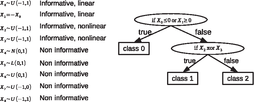We generated a continuous response by \documentclass{aastex}\usepackage{amsbsy}\usepackage{amsfonts}\usepackage{amssymb}\usepackage{bm}\usepackage{mathrsfs}\usepackage{pifont}\usepackage{stmaryrd}\usepackage{textcomp}\usepackage{portland, xspace}\usepackage{amsmath, amsxtra}\pagestyle{empty}\DeclareMathSizes{10}{9}{7}{6}\begin{document} $$Y = 2X_0^2 + X_3^2 + 10X_1 X_2$$ \end{document} , thus features X₀, X₁, X₂, and X₃ are informative ones, and X₄, X₅, and X₆ are noninformative ones. Ten thousand samples were generated. We apply quartiles to convert the continuous response to four classes.

FIG. 2.

Distributions of features and their relationships to class labels on Simulation1.

Each simulated data set was equally split to training, validation, and test sets in order to evaluate deep DFS, shallow DFS, LASSO (Tibshirani, 1996), and random forest (Breiman, 2001) for feature selection. The DFS models learned on a training set and used validation error to avoid overfitting. LASSO and random forest were learned on a training set. The accuracy of predicting the labels of test samples were used to measure the performance of a model. In the deep DFS model, we used three hidden layers ({36, 18, 9} neurons for Simulation1, and {28, 14, 7} neurons for Simulation2) with ReLU as activation functions, respectively. In both deep DFS and shallow DFS, we set the initial learning rate to 0.1, λ₂ = 1, α₁ = 0.0001, and α₂ = 0. We used values of λ₁ ranging from 0.05 to 0. We used the glmnet package (Friedman et al., 2010) for LASSO, and the randomForest package (Liaw and Wiener, 2002) for random forest.

We recorded weights of the features and corresponding test accuracies in Table 1. The results on Simulation1 is shown at the top of Table 1. We found that deep DFS are able to discover the linear features, X₀ and X₁, and the nonlinear features, X₂ and X₃. Using the linear features only, deep DFS obtained an accuracy of 0.6723. Adding the nonlinear features, deep DFS achieved an accuracy of 0.9907. From the experiment, we can see that the shallow DFS can only recover the linear features, X₀ and X₁. Thus, this model can only correctly predict the class labels of two thirds of the test samples. Consistent with common knowledge, LASSO tended to select only one of the correlated linear features. Its classification performance is similar to shallow DFS. From our results, we also found that the DFS models can select correlated features (X₀ and X₁) simultaneously, while LASSO only utilizes one of them. The last row of Table 1 shows the importance of features computed by random forest. We can see that random forest has the capability of identifying both linear and nonlinear features. The accuracies between deep DFS and random forest models were comparable.

Table 1.

Feature Weights (or Importance) and Corresponding Accuracies of Different Methods on Simulated Data

				Feature weight or importance
Data	Method	λ ₁	Accuracy	X0	X1	X2	X3	X4	X5	X6	X7	X8
Simulation1	Deep DFS	0.0059	0.6723	0.5895	0.9696	0.0001	0	0.0001	0	0	0	0
		0.0052	0.9970	0.8961	1.0138	1.6211	1.5099	0	0	−0.0003	0	0
		0	0.9907	2.3425	1.8052	2.9091	2.6366	0.7225	0.6456	0.5941	0.7496	0.7060
	Shallow DFS	0.0120	0.6653	1.6776	1.6776	0.0134	0.0004	0.0017	0	0.0037	−0.0066	0.0006
		0	0.6660	2.0793	2.0793	1.0016	0.9976	0.9754	0.9612	0.4666	0.4455	1.0027
	LASSO	0.01069	0.6603	3.9313	0	0.0042	0	0	0	0	0	0
		0.00557	0.6643	5.4498	0	0.0202	0	0.0015	0.0009	0.0108	0.0134	0.0031
		0.00004	0.6613	6	0	0.1337	0.0157	0.0693	0.0062	0.3013	0.2822	0.0385
	Random Forest	-	0.9983	0.1926	0.2197	0.1866	0.1859	0.0001	0.0001	−0.0004	−0.0005	0.0001
Simulation2	Deep DFS	0.0295	0.7346	1.0917	−0.0003	0.0009	-0.5270	−0.0006	0.0005	0	-	-
		0.0045	0.9780	3.3341	1.6364	1.7290	1.9035	0.0001	−0.0003	0	-	-
		0	0.9694	3.9363	2.0156	2.0792	2.3154	0.3874	−0.0811	0.9214	-	-
	Shallow DFS	0.010	0.6951	4.2636	−0.0002	1.4119	0	0.0002	0.0018	−0.0002	-	-
		0.007	0.7902	4.4530	0	1.6547	1.9026	0	0.3543	0	-	-
		0	0.7866	5.7071	1.1806	2.6090	2.8195	1.5737	1.3613	1.2327	-	-
	LASSO	0.10426	0.5780	3.6753	0	0	0.1704	0	0	0	-	-
		0.01227	0.8903	6	2.9065	4.6875	6	0	0	0	-	-
		0.00006	0.9025	6	6	6	6	0.3125	0.1208	0.5602	-	-
	Random Forest	-	0.8965	0.4347	0.0389	0.0847	0.1146	0.0013	0.0025	0.0025	-	-

Large nonzero numbers in a sparse vector are highlighted in boldface.

The bottom of Table 1 shows the results on Simulation2. Deep DFS was able to identify all informative features and obtained the highest accuracy (0.9780). Shallow DFS only obtained an accuracy of 0.7902 using four features. It correctly selected features used in squared terms, but failed to recover features interacting with others. LASSO could select all informative features but could not fully model the nonlinearity. It obtained an intermediate result (0.8903). Random forest had a similar accuracy to LASSO. It tended to give a much higher score to X₀, but underrepresented X₁, X₂, and X₃.

Overall, we conclude that deep DFS can identify informative features involved in nonlinear rules and polynomial terms. It highlights important features with stronger distinction; that is, the difference in feature weights between the informative features and the noninformative features was greater for deep DFS than random forest. Shallow DFS can only identify features related to linear rules and noninteractive polynomial terms, thus has low performance. LASSO fails to recover features involved in nonlinear rules. The importance scores of random forest reflect the usefulness of features, but are less distinctive than DFS. Random forest has a comparable accuracy on the data generated by nonlinear rules, but gets lower performance on the data generated using quadratic polynomial.

4. Applying DFS to Enhancer–Promoter Classification

We applied the DFS model in the challenging problem of enhancer–promoter classification. In order to assess the performance of this model, we compared four models, including our deep DFS model having two hidden layers (Fig. 1D), our shallow DFS model having no hidden layer (Fig. 1B), elastic-net-based softmax regression (Fig. 1A), and random forest (Breiman, 2001). We shall first describe the genomic data we used. Then, we compare the prediction accuracy. Finally, we provide new insights into the features selected.

4.1. Data

We compared the models on our processed data sampled from annotated DNA regions of GM12878 cell line (a lymphoblastoid cell line). This data set has 93 features and three classes, each of which contains 2,156 samples. Based on the FANTOM5 promoter and enhancer atlases (The FANTOM Consortium et al., 2014; Andersson et al., 2014), each sample comes from one of the three classes of annotated DNA regions including active enhancer regions, active promoter regions, and background. The background class is a pool of inactive enhancers, inactive promoters, active exons, and unknown regions. The features include cell-ubiquitous characteristics such as CpG-islands and evolutionary conservation Phastcons score, and cell-specific events including DNA-accessibility, histone modifications, and transcription factor binding sites captured by the ENCODE consortium using ChIP-seq techniques (The ENCODE Project Consortium, 2012). For a fair comparison, we split our data set equally into training set, validation set, and test set. All models were trained on the same training set. The validation accuracy is used to monitor the training of the DFS models to avoid overfitting. The same test set was blinded in the training of all three models, so the test accuracy was used to examine the quality of feature subsets.

4.2. Comparing test accuracy

In our deep DFS model, we take the structure of {93 → 93 → 128 → 64 → 3} by a manual rough model selection, due to a concern about the efficiency of automatic model selection for deep models. We used tangent activation functions. We set the minbatch size to 100, the maximum number of epochs to 1000, the initial learning rate s = 0.1, and the coefficient of momentum α = 0.1, λ₂ = 1, α₁ = 0.0001, and α₂ = 0. We conducted feature selection for values of λ₁ from the range of [0, 0.03] by a step of 0.0002. Our shallow DFS model has a structure of {93 → 93 → 3}. For this model, we tried values of λ₁ from [0, 0.07] by a step of 0.0005. The rest of the user-specified parameters were kept the same as the deep DFS above. Elastic-net-based softmax regression simply has a structure of {93 → 3}. We tried different values of α. We used the glmnet package for it, thus the full regularization path with a fixed value of α was produced by a cyclic coordinate descent algorithm (Friedman et al., 2010). For random forest, we applied the randomForest package in R (Liaw and Wiener, 2002).

The test accuracies versus the sizes of feature subsets are illustrated in Fig. 3A. From a feature selection context, we focus the comparison on the critical region as highlighted by a rectangle in this plot. In this region, the paired Wilcoxon signed-rank test was conducted to check whether a classifier significantly outperforms another one (see Fig. 3B). In addition to accuracy, the confusion matrices of different models, when selecting 16 features, are given in Figure 3C. First of all, with the comparison between our shallow DFS model and elastic net, it can be seen that our shallow model has a significantly higher test accuracy than elastic net for the same number of selected features. From a computational viewpoint, it hence corroborates that adding a sparse one-to-one layer is a better technique than the tradition of simply combining the feature subsets selected for each class. Second, from the comparison of our deep and shallow DFS models, it shows that a significantly better test accuracy can be obtained by our deep model. It hence supports that considering the nonlinearity among the variables can contribute to the improvement of prediction capability. Third, it is interesting to see that random forest with certain top-ranked features performs better than the deep learning model. This may be because the structure and parameter of the deep model was not optimized. Finally, from the confusion matrices as shown in Figure 3C, we highlight that some active promoters tend to be classified as active enhancers.

FIG. 3.

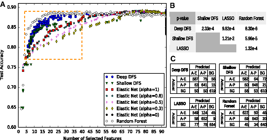
Comparison of classification performance on enhancer and promoter data. (A) The number of selected features by different methods and corresponding test accuracy. The critical region is highlighted by the orange rectangle. (B) p-Value of the paired Wilcoxon signed-rank test in the critical region. (C) Confusion matrices when selecting 16 features by different models, respectively. A-E, active enhancer; A-P, active promoter; BG, background.

4.3. Feature analysis

We analyzed the features selected by the DFS models, LASSO, and random forest. Regularization path (Tibshirani, 1996; Efron et al., 2004) is a well-known method to illustrate the importance of selected features through plotting coefficients in curves. However, it becomes less informative as the number of features increases. Thus, as shown in Figure 4, we instead use a heatmap representation of feature coefficients that is equivalent to the regularization path. Since LASSO is supposed to have three (each for a class) heatmaps, we combined them by taking the corresponding maximal absolute values of its coefficients. 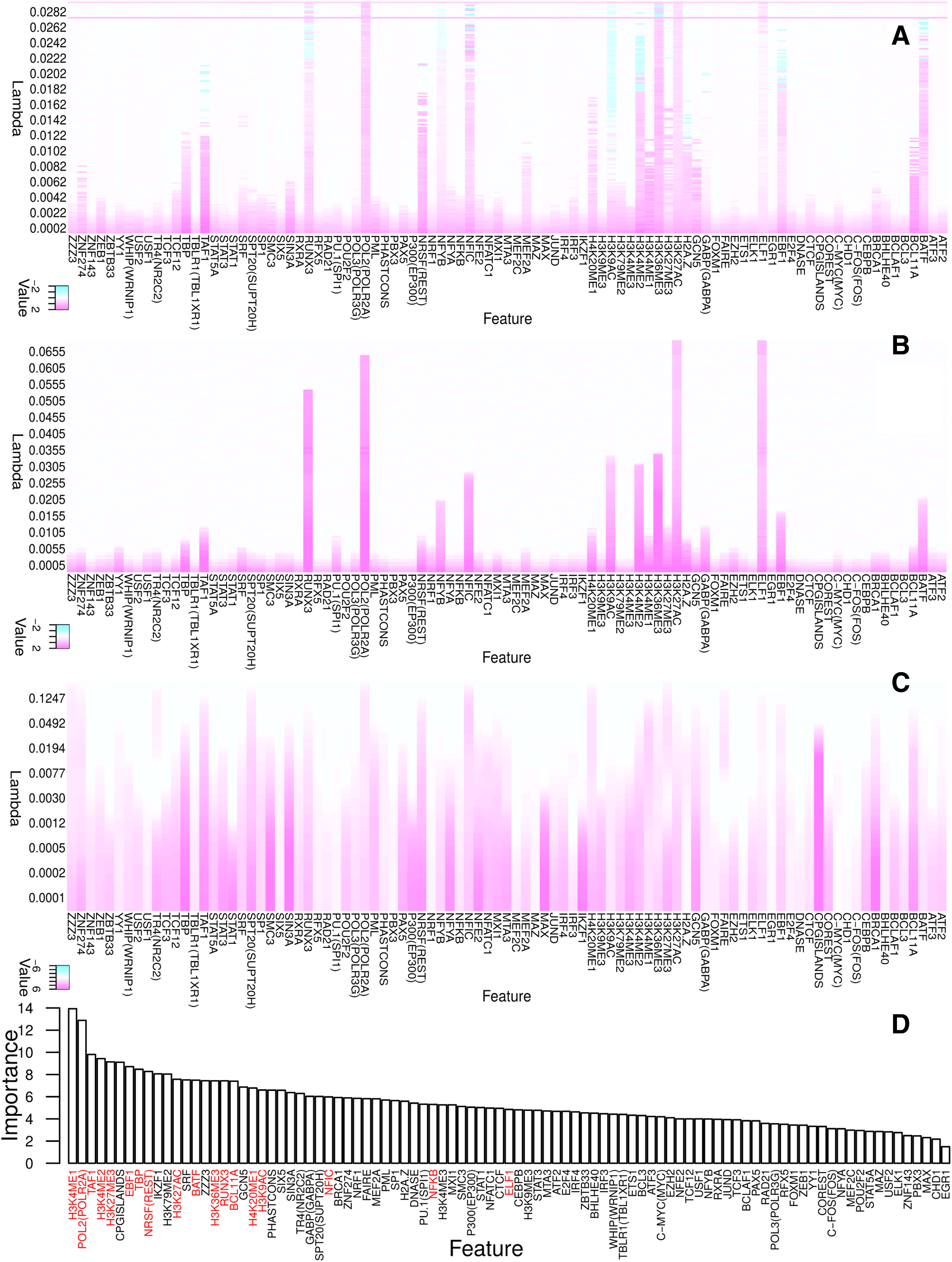That is, for a value of λ, we convert matrix W to a vector w ^new by \documentclass{aastex}\usepackage{amsbsy}\usepackage{amsfonts}\usepackage{amssymb}\usepackage{bm}\usepackage{mathrsfs}\usepackage{pifont}\usepackage{stmaryrd}\usepackage{textcomp}\usepackage{portland, xspace}\usepackage{amsmath, amsxtra}\pagestyle{empty}\DeclareMathSizes{10}{9}{7}{6}\begin{document} $$w_i^{{ \rm new}} = \max \{ \mid w_{i1} \mid , \mid w_{i2} \mid , \mid w_{i3} \mid \} $$ \end{document} .

FIG. 4.

Coefficient heatmaps (equivalent to the conventional regularization paths) of the DFS and LASSO models, and the importance of features ranked by random forest. (A) Coefficient heatmap of deep DFS. (B) Coefficient heatmap of shallow DFS. (C) Coefficient heatmap of LASSO. (D) Feature importances obtained by random forest. In the heatmaps, as the value of λ decreases vertically down, more and more coefficient becomes nonzero. The strength of the colors indicates the involvement of features in classification. The higher a bar is, the earlier the corresponding feature affects the classification. Eventually, all features turn to nonzero, affecting the classification. A pink horizontal line in (A) is because of a failure of the stochastic gradient descent algorithm, which can be overcome by a different initial solution. In (D), the key features listed in Table 2 are colored in red.

First, we can see that the heatmaps of our shallow and deep DFS models are much sparser than that of LASSO. This implies that our scheme using a sparse one-to-one weighting layer is able to select a small subset of features along the regularization path, while LASSO tends to select more features, because it fuses all class-specific feature subsets. Second, comparing the result of the shallow DFS and LASSO, we can see many differences. For example, LASSO emphasizes CpG islands, TBLP1, and TBP, while they are not selected by the shallow DFS until later in the process. Instead, the heatmap of the shallow DFS indicates that ELF1, H2K27ac, Pol2, RUNX3, etc., are important features.

From GeneCards (Rebhan et al., 1997) and literature, we surveyed the known functionality of features selected by the deep and shallow DFS in an early phase. The functionality and specificity of these features are given in Table 2, where the last column is our conclusion about the binding specificity of the features based on the box-plots (see Fig. 5) of our data. First, the table shows that deep DFS identifies more key features earlier than shallow DFS, such as BCL11A, HeK27me3, H3K4me1, H4K20me1, NRSF, TAF1, and TBP. Interestingly, the deep DFS found a nonlinear relation: TAF1 and TBP are actually components of TFIID functioning as RNA polymerase II locator. Second, we can see that the known functionality of the majority of selected features, as highlighted in bold in Table 2 (i.e., ELF1, H3K27ac, Pol2, BATF, EBF1, H3K36me3, H3K4me2, NFYB, RUNX3, BCL11A, H3K27me3, H3K4me1, and NRSF), are consistent with the binding specificity drawn from our data. From the box-plots of our data (Fig. 5), we are also able to identify novel enrichment of some features (emphasized by italic type in Table 2) in enhancers and inactive elements. For example, H3K9ac is thought to be enriched in actively transcribed promoters (Kratz et al., 2010); our results show that it is also enriched in active enhancers. H4K20me1 is reported to be enriched in exons (Vakoc et al., 2006); our results also show that both inactive enhancers and inactive promoters are enriched with H4K20me1. TAF1 and TBP is known as a promoter binder; our results show that they are also associated with active enhancers. Finally, it has to be mentioned that some cell-specific features can be identified by the DFS models. From Table 2, we can see that ELF1 (Bredemeier-Ernst et al., 1997), BATF (Ise et al., 2011), EBF1 (Nechanitzky et al., 2013), and BCL11A (Lee et al., 2013) are specific to lymphoid cells (recall that GM12878 is a lymphoblastoid cell line from blood). This further confirms that the selected features are highly informative.

FIG. 5.

Box plots of features selected by DFS in different classes. In addition, the last two features (CpGIslands and TBLR1) are the features selected by LASSO. The y axis is the fold change (experiment vs. input) of ChIP-seq signal. From the box plots, feature enrichment in different classes can be observed.

Table 2.

Key Features Selected by the Deep and Shallow DFS Models

Feature	Known functions	Specificity
ELF1	Primarily expressed in lymphoid cells. Binds to promoters and enhancers (Bredemeier-Ernst et al., 1997). Acts as both activator and repressor.	A-P, A-E
H3K27ac	Enriched in the flanking regions of active enhancers and active promoters (Shlyueva et al., 2014).	A-P, A-E
Pol2	Encodes RNA polymerase II to initialize transcription.	A-P
BATF	From AP-1/ATF superfamily. A negative regulator of AP-1/ATF transcriptional events. Interacts with Jun family to recognize immune-specific regulatory element. Binds to enhancers (Ise et al., 2011).	A-E
EBF1	Binds to enhancers of PAX5 for B lineage commitment (Nechanitzky et al., 2013).	A-E
H3K36me3	Enriched in transcribed gene body.	A-Ex
H3K4me2	Defines TF binding regions (Wang et al., 2014).	P, A-E
H3K9ac	Enriched in transcribed promoters (Kratz et al., 2010).	A-P, A-E
NFIC	Promoter binding transcription activator (Pjanic et al., 2011).	A-P, A-E
NFYB	Binds specifically to CCAAT motifs in the promoter regions.	A-P
RUNX3	Serves as both activator and repressor. Binds to a core DNA sequence of a number of enhancers and promoters.	A-P, A-E
BCL11A	Involved in lymphoma pathogenesis, leukemogenesis, and hematopoiesis. Binds to promoters and enhancers (Lee et al., 2013).	A-E, A-P
H3K27me3	Enriched in closed or poised enhancers (Shlyueva et al., 2014) and poised promoters (Zhou et al., 2011).	I-P, I-E
H3K4me1	Enriched in enhancer regions (Shlyueva et al., 2014).	A-E
H4K20me1	Enriched in exons (Vakoc et al., 2006).	A-Ex, I-P, I-E
NRSF/REST	Represses neuronal genes in non-neuronal tissues. With corepressors, recruits histone deacetylase to the promoters of REST-regulated genes.	A-P
TAF1	TAFs serve as coactivators. TAFs and TBP assemble TFIID to position RNA polymerase II to initialize transcription.	A-P, A-E
TBP	TATA-binding protein. Interacts with TAFs. Binds to core promoters.	A-P, A-E

The last column is the binding specificity of these features based on box-plots of our data (Fig. 5). Features consistent between known functions and binding specificity are highlighted in boldface. Features having novel enrichment are emphasized in italic type. A, active; I, inactive; P, promoter; E, enhancer; Ex, exon.

Random forest is suitable for multiclass data. It can return the importance of each feature by measuring the decrease of out-of-bag error by permuting the values of this feature (Breiman, 2001). We compared the features selected by our models with the ones ranked by random forest, as shown in Figure 4D. The majority of informative features selected by the DFS models are top-ranked in random forest, except that NFKB and ELF1 are scored as less important. It may be because our DFS model considers the dependency of the features, while random forest independently measures the impact of removing each feature from the model.

5. Computing Time

In Table 3, we recorded the training times of the four models tested on the synthetic and real data sets. Random forest and shallow DFS ran the fastest, taking a few seconds (even less than one second) to learn. Elastic net spent a few more seconds in training. The deep DFS model “unsurprisingly” consumed more time to finish the training procedure.

Table 3.

Comparison of Computing Times in Seconds

Data	Deep DFS	Shallow DFS	Elastic net	Random forest
Simulation1	18.38	0.99	4.67	0.62
Simulation2	5.57	3.71	8.08	0.75
Real	69.10	3.32	6.56	2.68

6. Conclusion and Future Works

Linear methods do not model the nonlinearity of variables and can not be extended to multiclass in a natural way for feature selection, while deep models learn nonlinearity and high-level representation of features. In this article, we propose a deep feature selection model for selecting input features in a deep structure, especially for multiclass data. We applied this model to distinguish active promoters and enhancers from the rest of the genome. Our results show that our shallow and deep DFS models are able to select a smaller subset of features than LASSO with comparable accuracy. Furthermore, our deep DFS can select discriminative features that may be overlooked by the shallow DFS. Through looking into the genomic features selected, we find that the features selected by DFS are biologically plausible. Furthermore, some selected features have novel enrichment in regulatory elements. We also evaluated the new model on simulated data in order to understand its behavior. Our results confirm that the deep DFS is able to recover both linear and nonlinear features. We implemented the DFS model in Python based on the Theano and Deep Learning Tutorials. This model together with our modification of the Deep Learning Tutorials led to a convenient deep learning package accessible at Li and Wyeth (2015).

More investigations should be conducted for improving the stability and performance of DFS. A few are enumerated below. First, we notice that the sign of weights in the one-to-one layer is not informative, because the sign can effectively be reversed by later layers. We thus plan to impose a non-negativity constraint on the weights of the one-to-one layer. Second, an observed limitation is the presence of negligible weights in the feature selection layer. Other sparse regularization techniques, for example, spike-and-slab (Goodfellow et al., 2012), can be tested to achieve a better quality of sparseness. Third, we note that DFS can be influenced by the purity of each minibatch. More research needs to be done to unveil the reason. Fourth, it is necessary to study whether there exists an efficient algorithm for computing the regularization path of the DFS model. Fifth, we will build a deep feature selection model to select variables for regression problems. We remain interested in devising feature selection methods for other deep learning models.

Footnotes

Acknowledgments

We thank the anonymous reviewers for constructive comments to improve the quality of this article. Dr. Anthony Mathelier (UBC) and Wenqiang Shi (UBC) provided valuable suggestions. Dr. Anshul Kundaje (Stanford) provided valuable instruction during the processing of ChIP-seq data from ENCODE. This research is supported by the Genome Canada Applied Bioinformatics of Cis-regulation for Disease Exploration project (ABC4DE, to ), the Natural Sciences and Engineering Research Council of Canada (NSERC) Postdoctoral Fellowship (PDF-471767-2015, to YL), and the UBC Four Year Doctoral Fellowship (to CYC).

Author Disclosure Statement

The authors declare that no competing financial interests exist.

References

Ackley

D.H.

, Hinton

G.E.

, and Sejnowski

T.J.

1985. A learning algorithm for Boltzmann machines. Cogn. Sci. 9, 147–169.

Andersson

, Gebhard

, Miguel-Escalada

, et al. 2014. An atlas of active enhancers across human cell types and tissues. Nature, 507, 455–461.

Bengio

, Courville

, and Vincent

2013. Representation learning: a review and new perspectives. IEEE Trans. Pattern Anal. Mach. Intell., 35, 1798–1828.

Bergstra

, Breuleux

, Bastien

, et al. 2010. Theano: a CPU and GPU math expression compiler, 1–7. In van der Walt

, and Millman

, eds. Proceedings of the Python for Scientific Computing Conference (SciPy), Austin, Texas.

Bradley

P.S.

, and Mangasarian

O.L.

1998. Feature selection via concave minimization and support vector machines, 82–90. In Shavlik

J.W.

, ed. Proceedings of the Fifteenth International Conference on Machine Learning. Morgan Kaufmann Publishers Inc., California.

Bredemeier-Ernst

, Nordheim

, and Janknecht

1997. Transcriptional activity and constitutive nuclear localization of the ETS protein Elf-1. FEBS Lett. 408, 47–51.

Breiman

2001. Random forests. Mach. Learn., 45, 5–32.

Cai

, Nie

, Huang

, et al. 2011. Multi-class l2,1-norm support vector machine, 91–100. In 19th IEEE International Conference on Data Mining. IEEE, IEEE Press, Piscataway, NJ.

Efron

, Hastie

, Johnstone

, et al. 2004. Least angle regression. Ann. Stat., 32, 407–499.

10.

Friedman

, Hastie

, and Tibshirani

2010. Regularization paths for generalized linear models via coordinate descent. J. Stat. Softw., 33, 1–22.

11.

Goodfellow

I.J.

, Courville

, and Bengio

2012. Large-scale feature learning with spike-and-slab sparse coding. International Conference on Machine Learning (ICML), pp. 1439–1446.

12.

Hinton

, and Salakhutdinov

2006. Reducing the dimensionality of data with neural networks. Science, 313, 504–507.

13.

Hinton

G.E.

, Osindero

, and Teh

2006. A fast learning algorithm for deep belief nets. Neural Comput. 18, 1527–1554.

14.

Ise

, Kohyama

, Schraml

B.U.

, et al. 2011. The transcription factor BATF controls the global regulators of class-switch recombination in both B cells and T cells. Nat. Immunol., 12, 536–543.

15.

Kong

, Ding

, and Huang

2011. Robust nonnegative matrix factorization using l21-norm, 673–682. In Berendt

, de Vries

, Fan

, et al., eds. Proceedings of the 20th ACM International Conference on Information and Knowledge Management. ACM Press, New York.

16.

Kratz

, Arner

, Saito

, et al. 2010. Core promoter structure and genomic context reflect histone 3 lysine 9 acetylation patterns. BMC Genomics. 11, 257.

17.

LeCun

, Bottou

, Bengio

, et al. 1998. Gradient-based learning applied to document recognition. Proc. IEEE, 86, 2278–2324.

18.

Lee

B.S.

, Dekker

J.D.

, Lee

B.K.

, et al. 2013. The BCL11A transcription factor directly activates rag gene expression and V(D)J recombination. Mol. Cell Biol., 33, 1768–1781.

19.

, and Ngom

2013. Classification approach based on non-negative least squares. Neurocomputing, 118, 41–57.

20.

, and Wyeth

W.W.

2015. DECRES: deep learning methods for identifying cis-regulatory elements and other applications. Available at: https://github.com/yifeng-li/DECRES

21.

Liaw

, and Wiener

2002. Classification and regression by randomForest. R News, 2, 18–22. Available at: http://cran.r-project.org/web/packages/randomForest

22.

LISA Lab. 2013. Deep learning tutorials. Available at: http://deeplearning.net/tutorial

23.

Nair

, and Hinton

2010. Rectified linear units improve restricted Boltzmann machines. IEEE International Conference on Machine Learning (ICML), Haifa, Israel, pp. 807–814.

24.

Nechanitzky

, Akbas

, Scherer

, et al. 2013. Transcription factor EBF1 is essential for the maintenance of B cell identity and prevention of alternative fates in committed cells. Nat. Immunol., 14, 867–875.

25.

Nie

, Huang

, Cai

, et al. 2010. Efficient and robust feature selection via joint l2,1-norms minimization, 1813–1821. In Lafferty

, Williams

, Shawe-Taylor

, et al., eds. Advances in Neural Information Processing Systems 23. Curran Associates Inc., New York.

26.

Pjanic

, Pjanic

, Schmid

, et al. 2011. Nuclear factor I revealed as family of promoter binding transcription activators. BMC Genomics, 12, 181.

27.

Rebhan

, Chalifa-Caspi

, Prilusky

, et al. 1997. GeneCards: integrating information about genes, proteins and diseases. Trends Genet. 13, 163.

28.

Sanders

2009. Sparse multi-class prediction based on the group lasso in multinomial logistic regression [Master's thesis]. Delft University of Technology, The Netherlands.

29.

Shlyueva

, Stampfel

, and Stark

2014. Transcriptional enhancers: from properties to genome-wide predictions. Nat. Rev. Genet., 15, 272–286.

30.

The ENCODE Project Consortium. 2012. An integrated encyclopedia of DNA elements in the human genome. Nature, 489, 57–74.

31.

The FANTOM Consortium, The RIKEN PMI, and CLST (DGT). 2014. A promoter-level mammalian expression atlas. Nature, 507, 462–470.

32.

Tibshirani

1996. Regression shrinkage and selection via the Lasso. J. R. Stat. Soc. Series B Stat. Methodol., 58, 267–288.

33.

Vakoc

C.R.

, Sachdeva

M.M.

, Wang

, et al. 2006. Profile of histone lysine methylation across transcribed mammalian chromatin. Mol. Cell. Biol., 26, 9185–9195.

34.

Wang

, Li

, and Hua

2014. H3K4me2 reliably defines transcription factor binding regions in different cells. Genomics, 103, 222–228.

35.

Zhou

V.M.

, Goren

, and Bernstein

B.E.

2011. Charting histone modifications and the functional organization of mammalian genomes. Nat. Rev. Genet., 12, 7–18.

36.

Zou

, and Hastie

2005. Regularization and variable selection via the elastic net. J. R. Stat. Soc. Series B Stat. Methodol., 67, 301–320.

Deep Feature Selection: Theory and Application to Identify Enhancers and Promoters

Abstract

Abstract

1. Introduction

2. Method

2.1. Deep feature selection

2.2. Learning model parameter

2.3. Shallow DFS is not equivalent to LASSO

2.4. Alternative: l2,1-norm based deep feature selection

3. Comparing Models on Synthetic Data

4. Applying DFS to Enhancer–Promoter Classification

4.1. Data

4.2. Comparing test accuracy

4.3. Feature analysis

5. Computing Time

6. Conclusion and Future Works

Footnotes

Acknowledgments

Author Disclosure Statement

References

2.4. Alternative: l_2,1-norm based deep feature selection