Gap Filling as Exact Path Length Problem

Abstract

One of the last steps in a genome assembly project is filling the gaps between consecutive contigs in the scaffolds. This problem can be naturally stated as finding an s-t path in a directed graph whose sum of arc costs belongs to a given range (the estimate on the gap length). Here s and t are any two contigs flanking a gap. This problem is known to be NP-hard in general. Here we derive a simpler dynamic programming solution than already known, pseudo-polynomial in the maximum value of the input range. We implemented various practical optimizations to it, and compared our exact gap-filling solution experimentally to popular gap-filling tools. Summing over all the bacterial assemblies considered in our experiments, we can in total fill 76% more gaps than the best previous tool, and the gaps filled by our method span 136% more sequence. Furthermore, the error level of the newly introduced sequence is comparable to that of the previous tools. The experiments also show that our exact approach does not easily scale to larger genomes, where the problem is in general difficult for all tools.

1. Introduction and Related Work

As high throughput sequencing has become a cheap and commonplace technology in modern biology, the genome of the studied organism has also become a fundamental resource for biological research. Even though the number of sequenced genomes has increased, many published genomes are in draft stage, meaning that the published sequence contains numerous gaps whose sequence is unknown. These gaps may correspond to important parts of the sequence and can limit the usability of the genome.

High-throughput sequencing technology cannot read the genome of an organism from the start to the end, but rather produces massive amounts of short reads. Genome assembly is the problem of reconstructing the genome from these short reads. In a typical genome assembly pipeline, the reads are first joined into longer contiguous sequences, called contigs. Using paired-end and mate pair reads, contigs are then organized into scaffolds, which are linear orderings of the contigs with the distance between consecutive contigs known approximately. In this work, we study the last stage in this pipeline, gap filling, where the gaps between consecutive contigs in scaffolds are filled by reusing the reads.

Many genome assemblers, like Allpaths-LG (Gnerre et al., 2011), ABySS (Simpson et al., 2009) and EULER (Pevzner and Tang, 2001), include a gap-filling module. There are also standalone gap-filling tools available, for example, SOAPdenovo's GapCloser (Luo et al., 2012) and GapFiller (Boetzer and Pirovano, 2012). All these tools attempt to identify a set of reads that could be used to fill the gap, and then perform local assembly on these reads. The local assembly methods vary from using overlaps between the reads in Allpaths-LG to using k-mer-based methods in GapFiller, or building a de Bruijn graph of the reads in SOAPdenovo's GapCloser. Some of these methods attempt to greedily find a filling sequence whose length approximately equals the gap length estimate, whereas others discard the length information. In order to identify the set of reads potentially filling the gap, these tools use the paired-end and mate pair reads having one end mapping to the flanking contigs. However, if the gap is long, paired-end reads might not span to the middle of the gap, while the coverage of mate pair reads may not be enough to close the gap. In a more theoretical study (Wetzel et al., 2011), the gap between two mates is considered as reconstructible if the shortest path in the assembly graph between the two flanking contigs is unique.

In this work, we formulate the gap-filling problem as the problem of finding a path of given length between two vertices of a graph [also called the exact path length (EPL) problem (Nykänen and Ukkonen, 2002)]. With respect to previous solutions, such a formulation allows us, on the one hand, to use all reads that are potentially useful in filling the gap, even if their pair does not map to one of the two flanking contigs. On the other hand, by solving this problem exactly, we do not lose paths that may have been ignored by a greedy visit of the graph.

The EPL problem is NP-hard in general, and we show that this is also the case with our variation for the gap-filling problem. Moreover, the EPL problem is known to be solvable in pseudo-polynomial time. We also show that the assembly graph instances are particularly easy by implementing a new and simpler dynamic programing (DP) algorithm and engineering an efficient visit of the entire assembly graph. This is based on restricting the visit only to those vertices reachable from the source vertex by a path of cost at most the upper-bound on the gap length. Moreover, our DP algorithm also counts the number of solution paths, information which might address some issues raised by Wetzel et al. (2011). We implemented the method in a tool called Gap2Seq and compared it experimentally to other standalone gap fillers on bacterial and human chromosome 14 data sets from GAGE (Salzberg et al., 2012) (thus, implicitly, also to the gap filling modules built into the assemblers). In total on the bacterial assemblies, we can fill 76% more gaps than the best of the previous tools, and the gaps filled by our method span 136% more sequence. Moreover, the error level of the newly introduced sequence is comparable to the previous tools. Our experiments on the GAGE assemblies of human chrromosome 14 show that our exact approach does not seem to scale easily to larger genomes. Even though more greedy approaches perform better on some assemblies, all tools have overall mixed results, underlining the difficulty of the problem on these instances. Gap2Seq is freely available online (Salmela et al., 2015).

2. Gap Filling as Exact Path Length Problem

2.1. Problem formulation

Let \documentclass{aastex}\usepackage{amsbsy}\usepackage{amsfonts}\usepackage{amssymb}\usepackage{bm}\usepackage{mathrsfs}\usepackage{pifont}\usepackage{stmaryrd}\usepackage{textcomp}\usepackage{portland, xspace}\usepackage{amsmath, amsxtra}\pagestyle{empty}\DeclareMathSizes{10}{9}{7}{6}\begin{document} $${ {\cal R}} = \{ R^1 , \ldots , R^n \} $$ \end{document} be the set of all sequencing reads. From these reads, and a pair of consecutive contigs S and T, one can build an assembly graph, and then try to find a path between the two contigs. This reconstruction phase can be guided by the constraint that the path length should match the gap length estimated in the scaffolding step. This problem is called gap filling. Figure 1 illustrates the setting.

FIG. 1.

Gap filling.

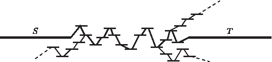
To state this problem more precisely, consider the formalism of the overlap graph G of \documentclass{aastex}\usepackage{amsbsy}\usepackage{amsfonts}\usepackage{amssymb}\usepackage{bm}\usepackage{mathrsfs}\usepackage{pifont}\usepackage{stmaryrd}\usepackage{textcomp}\usepackage{portland, xspace}\usepackage{amsmath, amsxtra}\pagestyle{empty}\DeclareMathSizes{10}{9}{7}{6}\begin{document} $${ {\cal R}}$$ \end{document} . This graph has a vertex i for every Rⁱ, and for every overlap between some Rⁱ and R^j, we add an arc (i, j). This arc is associated with the cost c(i, j) = |Rⁱ| – ℓ_i,j, where ℓ_i,j is the length of the longest suffix–prefix overlap between Rⁱ and R^j. In other words, c(i, j) is the length of the prefix of Rⁱ obtained by removing the longest overlap with R^j. Observe that we can assume that there are no 0-cost arcs in G, since this would indicate a read included in another read, which can be removed without changing the solution. In this article we allow paths to have repeated vertices, and we denote a path from a vertex u to a vertex v as a u-v path.

A path v₁,v₂,…,v_k in G spells a string of length \documentclass{aastex}\usepackage{amsbsy}\usepackage{amsfonts}\usepackage{amssymb}\usepackage{bm}\usepackage{mathrsfs}\usepackage{pifont}\usepackage{stmaryrd}\usepackage{textcomp}\usepackage{portland, xspace}\usepackage{amsmath, amsxtra}\pagestyle{empty}\DeclareMathSizes{10}{9}{7}{6}\begin{document} $$\sum \nolimits_{i = 1}^{k - 1} c ( v_i , v_{i + 1} ) + \mid R^{v_k} \mid$$ \end{document} , obtained by concatenating, for i from 1 to k − 1, the prefixes of length \documentclass{aastex}\usepackage{amsbsy}\usepackage{amsfonts}\usepackage{amssymb}\usepackage{bm}\usepackage{mathrsfs}\usepackage{pifont}\usepackage{stmaryrd}\usepackage{textcomp}\usepackage{portland, xspace}\usepackage{amsmath, amsxtra}\pagestyle{empty}\DeclareMathSizes{10}{9}{7}{6}\begin{document} $$c ( v_i , v_{i + 1} ) = \mid R^{v_i} \mid - \ell_{v_i , v_{i + 1}}$$ \end{document} of Rⁱ, followed by the last read \documentclass{aastex}\usepackage{amsbsy}\usepackage{amsfonts}\usepackage{amssymb}\usepackage{bm}\usepackage{mathrsfs}\usepackage{pifont}\usepackage{stmaryrd}\usepackage{textcomp}\usepackage{portland, xspace}\usepackage{amsmath, amsxtra}\pagestyle{empty}\DeclareMathSizes{10}{9}{7}{6}\begin{document} $$R^{v_k}$$ \end{document} .

Given a path P = v₁,v₂,…,v_k, with source s = v₁ denoting start contig S and sink t = v_k denoting end contig T, we say that the cost of P is cost(P) \documentclass{aastex}\usepackage{amsbsy}\usepackage{amsfonts}\usepackage{amssymb}\usepackage{bm}\usepackage{mathrsfs}\usepackage{pifont}\usepackage{stmaryrd}\usepackage{textcomp}\usepackage{portland, xspace}\usepackage{amsmath, amsxtra}\pagestyle{empty}\DeclareMathSizes{10}{9}{7}{6}\begin{document} $$ = \sum \nolimits_{i = 1}^{k - 1} c ( v_i , v_{i + 1} )$$ \end{document} ; namely, the cost of P is equal to the length of the string spelled by P starting with the string S, until the position immediately preceding T.

We formulate the gap-filling problem below by requiring that the cost of a solution path belongs to a given interval [d′, d]. In practice, d′ and d should be chosen such that the midpoint (d′ + d)/2 reflects the same distance as the length of the gap between S and T, estimated from the scaffolding step.

Problem 1 (Gap Filling) Given a directed graph G = (V,E), a cost function on its arcs \documentclass{aastex}\usepackage{amsbsy}\usepackage{amsfonts}\usepackage{amssymb}\usepackage{bm}\usepackage{mathrsfs}\usepackage{pifont}\usepackage{stmaryrd}\usepackage{textcomp}\usepackage{portland, xspace}\usepackage{amsmath, amsxtra}\pagestyle{empty}\DeclareMathSizes{10}{9}{7}{6}\begin{document} $$c : E \rightarrow {\mathbb Z}_{+}$$ \end{document} , and two of its vertices s and t, for all x in a given interval of path costs [d′,d], decide if there is a path P = v₁,v₂,…,v_k such that v₁ = s, v_k = t, and \documentclass{aastex}\usepackage{amsbsy}\usepackage{amsfonts}\usepackage{amssymb}\usepackage{bm}\usepackage{mathrsfs}\usepackage{pifont}\usepackage{stmaryrd}\usepackage{textcomp}\usepackage{portland, xspace}\usepackage{amsmath, amsxtra}\pagestyle{empty}\DeclareMathSizes{10}{9}{7}{6}\begin{document} \begin{align*}{\rm cost}\, ( P ) = \mathop \sum \limits_{i = 1}^{k - 1} c ( v_i , v_{i + 1} ) = x ,\end{align*} \end{document}

and return one such path if the answer is positive.

We denote by #Gap Filling the corresponding counting problem, which, for all x in the given interval of path costs [d′, d], counts the number of s-t paths of cost x.

2.2. Complexity and the pseudo-polynomial algorithm

The problem of finding a path P in a directed graph with integer arc costs, such that the cost of P equals an integer d given in input was studied by Nykänen and Ukkonen (2002). In fact, Nykänen and Ukkonen (2002) considered the more general version in which the arc costs can also be negative. They showed this problem to be NP-hard, even when restricted to DAGs, and only with nonnegative costs. Their reduction is from the Subset Sum problem (also called 0/1 Knapsack problem) (Garey and Johnson, 1979; Karp, 1972), consisting of a DAG with some 0-cost arcs. With a simple modification, we adapt it below to show that both the Gap Filling problem (with only positive costs) and its counting version are hard.

Theorem 2 The Gap Filling problem is NP-hard, and the #Gap Filling problem is #P-complete, even when restricted to DAGs without parallel arcs.

Proof. As in Nykänen and Ukkonen (2002), given an instance \documentclass{aastex}\usepackage{amsbsy}\usepackage{amsfonts}\usepackage{amssymb}\usepackage{bm}\usepackage{mathrsfs}\usepackage{pifont}\usepackage{stmaryrd}\usepackage{textcomp}\usepackage{portland, xspace}\usepackage{amsmath, amsxtra}\pagestyle{empty}\DeclareMathSizes{10}{9}{7}{6}\begin{document} $$A = \{ w_1 , \ldots , w_n \} $$ \end{document} and d to the Subset Sum problem (for deciding whether there is a subset of A of sum exactly d) we construct the DAG having \documentclass{aastex}\usepackage{amsbsy}\usepackage{amsfonts}\usepackage{amssymb}\usepackage{bm}\usepackage{mathrsfs}\usepackage{pifont}\usepackage{stmaryrd}\usepackage{textcomp}\usepackage{portland, xspace}\usepackage{amsmath, amsxtra}\pagestyle{empty}\DeclareMathSizes{10}{9}{7}{6}\begin{document} $$\{ v_0 , \ldots , v_n , u_1 , \ldots , u_n \} $$ \end{document} as vertex set, and choose s = v₀, t = v_n (see Fig. 2). For each i ∈[1, n], we add the arcs \documentclass{aastex}\usepackage{amsbsy}\usepackage{amsfonts}\usepackage{amssymb}\usepackage{bm}\usepackage{mathrsfs}\usepackage{pifont}\usepackage{stmaryrd}\usepackage{textcomp}\usepackage{portland, xspace}\usepackage{amsmath, amsxtra}\pagestyle{empty}\DeclareMathSizes{10}{9}{7}{6}\begin{document} $$( v_{i - 1} , v_i )$$ \end{document} , with cost w_i + 2, and \documentclass{aastex}\usepackage{amsbsy}\usepackage{amsfonts}\usepackage{amssymb}\usepackage{bm}\usepackage{mathrsfs}\usepackage{pifont}\usepackage{stmaryrd}\usepackage{textcomp}\usepackage{portland, xspace}\usepackage{amsmath, amsxtra}\pagestyle{empty}\DeclareMathSizes{10}{9}{7}{6}\begin{document} $$( v_{i - 1} , u_i )$$ \end{document} and (u_i, v_i), with cost 1. We have that the Subset Sum problem admits a solution of cost d if and only if the Gap Filling problem has an s-t path of cost in the interval [d + 2n, d + 2n]. Since the #Subset Sum problem is #P-complete (Dyer et al., 1993), this implies that also the #Gap Filling problem is #P-complete. ■

FIG. 2.

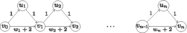
Reduction of a Subset Sum instance to a Gap Filling instance.

Nykänen and Ukkonen (2002) also gave a pseudo–polynomial time algorithm running in time O(W²n³ + |d| min(|d|,W)n²), where n is the number of vertices of the graph and W is the maximum absolute value of the arc costs. (This algorithm is called pseudo-polynomial because if the input integers W and d are assumed to be bounded by a polynomial in the input size, then it runs in polynomial time.)

However, the Gap Filling problem is easier, since the costs are only positive. As such, we can derive a much simpler algorithm, with running time O(dm) where m is the number of arcs in the graph. This algorithm is based on the classical pseudo-polynomial dynamic programming for the Subset Sum problem. We present this algorithm for the counting version of the problem, and then show how it can be easily adapted for Gap Filling.

Let N^– (v) denote the set of in-neighbors of v in V (G), that is, \documentclass{aastex}\usepackage{amsbsy}\usepackage{amsfonts}\usepackage{amssymb}\usepackage{bm}\usepackage{mathrsfs}\usepackage{pifont}\usepackage{stmaryrd}\usepackage{textcomp}\usepackage{portland, xspace}\usepackage{amsmath, amsxtra}\pagestyle{empty}\DeclareMathSizes{10}{9}{7}{6}\begin{document} $$N^{ -} ( v ) = \{ u \,\mid \,( u , v ) \in E ( G ) \} $$ \end{document} . We define, for all v ∈V (G), and ℓ ∈[0,d], \documentclass{aastex}\usepackage{amsbsy}\usepackage{amsfonts}\usepackage{amssymb}\usepackage{bm}\usepackage{mathrsfs}\usepackage{pifont}\usepackage{stmaryrd}\usepackage{textcomp}\usepackage{portland, xspace}\usepackage{amsmath, amsxtra}\pagestyle{empty}\DeclareMathSizes{10}{9}{7}{6}\begin{document} \begin{align*}a ( v , \ell ) = { \rm number \ of} \ s-v \ { \rm paths \ of \ cost} \ exactly \ \ell.\end{align*} \end{document}

We initialize a(s, 0) = 1, a(v, 0) = 0 for all v ∈V (G)\{s}, and a(v, ℓ) = 0 for all v ∈V (G) and ℓ < 0. The values a(·,·) can be computed by dynamic programming using the recurrence \documentclass{aastex}\usepackage{amsbsy}\usepackage{amsfonts}\usepackage{amssymb}\usepackage{bm}\usepackage{mathrsfs}\usepackage{pifont}\usepackage{stmaryrd}\usepackage{textcomp}\usepackage{portland, xspace}\usepackage{amsmath, amsxtra}\pagestyle{empty}\DeclareMathSizes{10}{9}{7}{6}\begin{document} \begin{align*}a ( v , \ell ) = \sum \limits_{u \in N^{ -} ( v ) } a ( u , \ell - c ( u , v ) ) \tag{1}\end{align*} \end{document}

The values a(·,·) can be computed by filling a table A[1, |V |][0, d] column-by-column. Let m denote the number of arcs of the graph. This DP computation can be done with O(dm) arithmetic operations, since for each ℓ ∈[0, d], each arc is inspected only once. The gap-filling problem admits a solution if there exists some ℓ ∈[d′, d] such that a(t, ℓ) ≥ 1. One solution path can be traced back by repeatedly selecting the in-neighbor of the current vertex that contributed to the sum in Equation (1).

Observe that, since there are O(m^d) s-t paths of length d, then the numbers a(·,·) need at most d log m bits, and each arithmetic operation on such numbers takes time O(d log m). Therefore, we have the following result.

Theorem 3 The #Gap Filling problem can be solved using O(d²m log m) bit operations, where m is the number of arcs of the graph, and d is the maximum path cost.

For the Gap-Filling problem itself, instead of storing counts, one can just fill in the binary information that tells whether there is a path of given length [and by replacing the summation operation by the “or” operation in Equation (1)]. This simplified solution leads to the following result.

Theorem 4 The Gap-Filling problem can be solved in time O(dm), where m is the number of arcs of the graph, and d is the maximum path cost.

Remark 5 Observe that, in practice, the maximum gap length estimate d is in fact smaller than the total number of reads that is n. For this reason, both dynamic programming algorithms do run in time polynomial in n.

Remark 6 The above dynamic programming algorithms can be easily extended to the more general problem considered by Nykänen and Ukkonen (2002), which allows negative arc costs. Then, just like in the Bellman-Ford algorithm (Bellman, 1958), we need to add another parameter to the dynamic programming recurrence, namely the number of arcs on an s-v path of specified length. Since now an s-t path can use at most md arcs, then this leads—for example, for the Gap Filling problem—to an algorithm working in time O(d²m²).

3. Engineered Implementation

In this section we describe an efficient implementation of the above gap-filling algorithm. In particular, we show how to reduce the above complexity O(dm), where m is the number of arcs of the entire assembly graph, down to O(dm′), with a meet in the middle strategy such that m′ can be much smaller than m. Namely, m′ is now the number of arcs of the assembly graph on the union of all paths starting at s and of cost at most d/2 and of all paths starting at t and of cost at most d/2 on the graph with reversed arcs. A similar meet in the middle approach has been proposed by Jackman et al. (2015).

We first describe a simplified variant of our actual implementation, which achieves the same complexity but is easier to describe in detail. Then we sketch how our implementation differs from this.

We use a de Bruijn graph (DBG) as the assembly graph. The DBG of a set of reads is a graph where each k-mer occuring in the reads is a vertex and there is an arc between two vertices if the k-mers overlap by k – 1 bases. Conceptually, a DBG can be thought of as a special case of an overlap graph where the reads are of length k and an arc is added only for overlaps of length k – 1. We implemented DBGs using the Genome Assembly and Analysis Tool Box (GATB) (Drezen et al., 2014), which includes a low memory implementation. By default, we set k = 31, which works well for bacterial genomes, but for larger genomes a larger k should be chosen.

We build the DBG of the whole read set. To leave out erroneous k-mers, only k-mers that occur at least r times in the reads are included (by default r = 2). The computation for each gap will then be performed on the appropriate subgraph of this DBG.

The gap-filling subroutine takes as input the bounds on the length of the gap, d′ and d, and the left and right k-mers flanking the gap, which will be the source and target vertices in our computation. We start a breadth-first search from the target vertex backward toward the source vertex to discover vertices that can reach the target within the allowed maximum gap length divided by two. We mark all vertices reached in this initial backward traversal. Then we continue with another breadth-first search from the source vertex forward toward the target vertex to discover vertices that are reachable from the source within the allowed maximum gap length divided by two. After reaching this limit, we continue the forward traversal only on the marked vertices; we then know that unmarked vertices do not belong to an s-t path of length at most d.

We note that this latter search traverses the vertices in an order that corresponds to the column-by-column filling of the DP table A defined in the previous section. Therefore the computations can be interleaved, resulting in an outer loop on the distance from the source vertex, and an inner loop on vertices at a specific distance from the source.

We use a hash table to link the reachable vertices to their DP table rows. The rows of the DP table may be sparse, since not all path lengths are necessarily feasible. For example, in the S. aureus test data with scaffolds constructed by SGA (Simpson and Durbin, 2012), 92% of the entries in the entire table were zero. We exploit this sparsity simply by listing all nonzero entries in every row. Because of the breadth-first search, the entries are added so that the lists will be sorted by the distance from the source vertex. Since we use a DBG, we always use the current distance minus one when accessing the table A, so we are only accessing the two last elements in the list. Therefore, this access can be implemented in constant time resulting in the O(dm′) complexity of the algorithm as claimed above. However, for tracing back the solution, one needs to binary search the corresponding elements. Hashing could be used for avoiding the binary search, but since tracing back is a negligible part of the total running time, this optimization was not implemented.

It is possible that there are several paths between the source and the target vertices. We then need to choose one of them to recover the sequence that will close the gap. We first choose paths whose length is closest to the estimated gap length. If there are still multiple possible paths, our current implementation chooses a random feasible in-neighbor when tracing back in the DP table.

Sometimes the k-mers immediately flanking gaps are erroneous (Boetzer and Pirovano, 2012). To be more robust, we allow paths to start or end at up to e of the k-mers that flank the gap (by default e = 10). This can be easily implemented by counting the length of a path always from the left-most possible starting k-mer. In the first e rounds of the breadth first search we add the appropriate starting k-mer to the reachable set with the number of paths equal to 1 at that distance. The searched path lengths can now be 2e bases longer, and we need to search for the ending right k-mer among the first e k-mers after the gap.

Observe that instead of just marking the reached vertices on the backward traversal, one can readily fill a DP table corresponding to the reverse paths. Then the forward traversal and DP computation can be stopped at level d/2, and the results of these two DP tables can be combined. This is the variant we actually implemented. Note that this approach is analogous to the standard dynamic programming technique known as forward and backward algorithms in HMM parameter estimation (Durbin et al., 1998).

Our implementation allows parallel gap filling on the scaffold level. We also utilize a limit on the memory usage of the DP table. If this limit is exceeded before a path is found, we abandon the search.

4. Experimental Setup

We evaluated our tool Gap2Seq against GapFiller (Boetzer and Pirovano, 2012) and SOAPdenovo's (Luo et al. (2012)) stand-alone tool GapCloser. For the experimental evaluation we used the GAGE (Salzberg et al., 2012) data sets Staphylococcus aureus, Rhodobacter sphaeroides, and human chromosome 14 (hereafter named staph, rhodo, and human14, respectively) using a wide range of assemblers. The details of the read sets available to gap fillers are shown in Table 1. For details of the different assemblies we refer the reader to GAGE (Salzberg et al., 2012). Since gaps tend to be introduced in complex areas (e.g., repeated regions or low coverage areas), it is important to evaluate the quality of the sequence inserted by a tool, in addition to the number and length of gaps filled. The quality of the scaffolds on the original assembly as well as of the gap-filled scaffolds was assessed using QUAST (Gurevich et al., 2013). QUAST evaluates assemblies by parsing nucmer (Kurtz et al., 2004) alignments computed between the assembly and the reference sequence.

Table 1.

Read Data Sets Used in the Evaluation

Organism	Library	Mean insert size	SD of insert size	Read length	Coverage
Staph	Short frag	180	30	101	45×
Staph	Long frag	3500	300	37	45×
Rhodo	Short frag	180	30	101	45×
Rhodo	Long frag	3500	300	101	45×
Human14	Short frag	155	20	101	42×
Human14	Long frag	2500	381	101	26×

Gap2Seq v1.0, GapFiller v1.10, and GapCloser v1.12 were run with default parameters on a 32 GB RAM machine equipped with 8 cores. Table 2 summarizes the parameters used by Gap2Seq. GapFiller v1.10 is coupled with BWA (Li and Durbin, 2009) v0.5.9 and with Bowtie (Langmead et al., 2009) v0.12.5. We used both aligners in the evaluation. To better evaluate the gap-filling results, we modified the output produced by QUAST v2.3 with respect to the classification of “misassemblies” and local “misassemblies.” Consider a scaffold ABC (consisting of subsequences A, B, and C) where sequence B is misplaced. Originally, QUAST would give in this case two breakpoints (between AB and BC respectively), thus two misassemblies would be reported. If both the length of B, and the distance between A and C, are shorter than Nbp (suggesting a local erroneous inserted sequence), we instead classify it as one local misassembly and compute its length. We chose N = 4000, since it is a rough upper bound of the insert size of the mate pair libraries. Thus, gaps are not expected to be longer than this. This change implies that we can measure in more detail the size of the erroneous sequences instead of simply classifying them as misassembly errors.

Table 2.

Parameters of Gap2Seq

Parameter	Default	Description
-k < k >	31	The length of k-mers in the DBG. The default value is good for bacterial data, but for larger genomes a larger value should be used. We used k = 61 for the human chromosome 14 data.
-solid < r >	2	The threshold for the number of times a k-mer has to occur in the input reads to be included in the DBG. Some gaps in scaffolds are due to low coverage of sequencing. Therefore we chose to set this parameter low.
-dist-error < (d − d′)/2 >	500	The maximum error in gap length estimates in bp. We consider 500 bp to be a safe maximum error but for assemblies with very poor gap length estimates this parameter may need to be increased.
-fuz < e >	10	The maximum number of nucleotides that can be ignored by the path search on the flanking contigs. One should consider increasing this parameter for assemblies with poor quality on the contig flanks. However, increasing this parameter also increases the length of the gap to be spanned by path search, which in turn increases the complexity of filling the gap. Therefore, we decided to keep the value of this parameter low.
-max-mem < m >	20	The maximum memory used for the DP tables by all threads. Note that increasing the available memory can also make Gap2Seq slower, because it takes longer to run out of resources on particularly difficult gaps.
-nb-cores < p >	0	The number of threads launched. The default value 0 allows Gap2Seq to use all available cores.

For each assembly, we used our modified version of QUAST to compute:

1. Misassemblies: The number of misassembled sequences in a scaffold that are larger than Nbp.

2. Erroneous length: Total length of erroneous sequence: the sum of lengths of all mismatches, indels, and local misassemblies (mismatches have length 1).

3. Unaligned length: The total length of the unaligned sequence in an assembly.

4. NGA50: NG50 is the size of the longest scaffold such that the sum of the lengths of all scaffolds longer than it is at least half of the (known) reference genome size. NGA50 is the NG50 after scaffolds have been broken at every position where a local misassembly or misassembly has been found.

5. Number of gaps: The number of sites with one or more unknown position(s) (that is, labeled “N”).

6. Total gap length: The sum of all lengths of the sites with one or more “N's.”

5. Discussion

5.1. Bacterial data sets

Tables 3 and 4 present the gap-filling performance for the bacterial data sets provided by GAGE. With the evaluation metrics introduced in the previous section, Gap2Seq produces favorable results. Gap2Seq is able to close more and longer gapped sequences in almost all cases. For example, on the ABySS, ABySS2, Allpaths-LG, and SOAPdenovo assemblies, Gap2Seq closes more than 90% of the total gap length, which is a large improvement over GapCloser and GapFiller. In the rhodo data set, Gap2Seq closes on average 25% of the total gap length, but it performs in general more than twice as well as the other two tools. Moreover, for both datasets there is no general increase in misassembled sequences. In fact, in total Gap2Seq also has the highest NGA50 on both genomes. We see that the results on these data sets support a general gain in quality from gap filling and thus, the motivation for using Gap2Seq.

Table 3.

Quality of Original and of the Gap-filled Assemblies on Staph

Tool	Original	GapCloser	GapFiller-bowtie	GapFiller-bwa	Gap2Seq
ABySS
Misassemblies	5	+0%	+0%	−40%	+60%
Erroneous length	10587	+27.5%	−3.5%	+12.5%	+70.5%
Unaligned length	7935	−19.8%	−10.2%	−10.2%	−43.0%
NGA50	31079	+0%	+0%	+0.3%	+0.3%
Number of gaps	69	−15.9%	−13.0%	−30.4%	−87.0%
Total gap length	55885	−25.3%	−9.5%	−23.3%	−94.5%
ABySS2
Misassemblies	5	+20%	+0%	+60%	+40%
Erroneous length	10312	−4.7%	+0.5%	−28.7%	−27.4%
Unaligned length	0	+0	+0	+0	+0
NGA50	106796	+15.1%	+0%	+0%	+29.0%
Number of gaps	35	−25.7%	−11.4%	−37.1%	−80%
Total gap length	9393	−63.3%	−29.9%	−58.6%	−94.5%
Allpaths-LG
Misassemblies	0	+0	+1	+1	+0
Erroneous length	5991	−22.7%	−5.9%	−14.0%	+9.7%
Unaligned length	0	+0	+0	+0	+0
NGA50	110168	+2.7%	+35.9%	+69.6%	+48.5%
Number of gaps	48	−47.9%	−31.2%	−41.7%	−70.8%
Total gap length	9900	−74.4%	−23.1%	−41.1%	−94.7%
Bambus2
Misassemblies	0	+1	+0	+0	+0
Erroneous length	24570	−23.0%	−4.4%	+16.5%	−1.4%
Unaligned length	0	+0	+0	+0	+0
NGA50	40233	+39.0%	+1.6%	+7.3%	+17.2%
Number of gaps	99	−68.7%	−14.1%	−19.2%	−69.7%
Total gap length	29205	−77.1%	−23.9%	−39.5%	−84.1%
MSR-CA
Misassemblies	10	−30%	−30%	−30%	−20%
Erroneous length	17276	−2.7%	−0.3%	+1.7%	−4.0%
Unaligned length	0	+0	+0	+0	+0
NGA50	64114	+50.3%	+20.4%	+20.4%	+50.3%
Number of gaps	81	−51.9%	−19.8%	−30.9%	−56.8%
Total gap length	10353	−75.6%	−24.5%	−39.4%	−70.5%
SGA
Misassemblies	2	+0%	+0%	+0%	−50%
Erroneous length	13811	−42.7%	−19.9%	−29.8%	−10.6%
Unaligned length	0	+0	+0	+0	+0
NGA50	9541	+148.1%	+8.9%	+10.3%	+221.4%
Number of gaps	654	−74.8%	−20.8%	−37.5%	−80.1%
Total gap length	300607	−53.8%	−5.7%	−10.3%	−72.1%
SOAPdenovo
Misassemblies	2	+0%	+0%	+0%	+0%
Erroneous length	35433	−1.3%	+1.2%	+0.7%	−1.5%
Unaligned length	4055	−100%	−100%	−100%	+3.9%
NGA50	69834	+0%	+0%	+0%	+0%
Number of gaps	9	−22.2%	−22.2%	−33.3%	−55.6%
Total gap length	4857	−61.4%	−24.0%	−38.2%	−94.2%
Velvet
Misassemblies	25	+8%	+0%	+4%	+8%
Erroneous length	24160	−32.1%	−2.2%	−19.6%	−36.3%
Unaligned length	1270	−49.4%	−20.5%	−21.3%	−49.4%
NGA50	46087	+19.1%	+26.0%	+49.0%	+73.3%
Number of gaps	128	−46.9%	−30.5%	−39.8%	−68.8%
Total gap length	17688	−59.6%	−37.9%	−47.6%	−81.2%
TOTAL
Misassemblies	49	+2.0%	−4.1%	+0%	+8.2%
Erroneous length	142140	−13.5%	−3.3%	−4.7%	−4.6%
Unaligned length	13260	−47.2%	−38.7%	−38.7%	−29.2%
NGA50	477852	+18.8%	+13.8%	+24.4%	+37.4%
Number of gaps	1123	−62.7%	−20.9%	−35.4%	−76.0%
Total gap length	437888	−53.2%	−10.3%	−18.1%	−77.3%

The results shown are relative differences with respect to the results of the original assembly. The bottom section of the table (TOTAL) is obtained by summing up the results of each gap filler for all assemblies. For each row, the best result is bolded and the worst result is shown in italics.

Table 4.

Quality of Original and of the Gap-Filled Assemblies on Rhodo

Tool	Original	GapCloser	GapFiller-bowtie	GapFiller-bwa	Gap2Seq
ABySS
Misassemblies	20	+0%	+0%	+0%	+5%
Erroneous length	140634	+0.7%	−2.5%	−0.8%	−0.4%
Unaligned length	23522	−9.8%	+100.9%	+83.1%	−10.0%
NGA50	6538	+0.7%	+0.6%	+0.2%	+4.4%
Number of gaps	323	−6.5%	−8.7%	−20.7%	−45.8%
Total gap length	114587	−5.0%	−0.3%	−3.8%	−19.6%
ABySS2
Misassemblies	12	+16.7%	+0%	+0%	+133.3%
Erroneous length	15750	+31.5%	−0.4%	+0.5%	+38.5%
Unaligned length	8230	−1.1%	−1.9%	−36.1%	+0%
NGA50	31197	+13.7%	−0.0%	+3.8%	+11.1%
Number of gaps	292	−4.1%	−1.4%	−5.8%	−19.9%
Total gap length	62627	−15.3%	+2.6%	−8.6%	−38.7%
Allpaths-LG
Misassemblies	5	+20%	+0%	+0%	+0%
Erroneous length	11738	+97.1%	−2.6%	−2.0%	+3.4%
Unaligned length	0	+0	+0	+0	+0
NGA50	79634	+11.5%	+2.0%	−0.0%	+12.8%
Number of gaps	170	−3.5%	−3.5%	−3.5%	−9.4%
Total gap length	21409	−13.4%	+8.0%	+0.9%	−25.0%
Bambus2
Misassemblies	5	+0%	+0%	+0%	+0%
Erroneous length	106359	+0.6%	−0.6%	−0.8%	+0.5%
Unaligned length	4716	−0.7%	−2.7%	−5.5%	−100%
NGA50	15043	+0%	+0%	+0%	+1.3%
Number of gaps	85	−10.6%	−5.9%	−7.1%	−35.3%
Total gap length	57041	−11.0%	−9.6%	−14.1%	−31.9%
CABOG
Misassemblies	15	+0%	+0%	−13.3%	−13.3%
Erroneous length	16750	+43.2%	+0.3%	+0.3%	−1.9%
Unaligned length	0	+0	+0	+0	+0
NGA50	26819	+3.5%	+11.4%	+11.4%	+3.9%
Number of gaps	193	−4.1%	−2.1%	−4.7%	−9.3%
Total gap length	21547	−17.9%	+5.7%	−3.9%	−22.5%
MSR-CA
Misassemblies	10	+20%	+0%	+0%	+270%
Erroneous length	22522	−7.1%	+2.6%	+8.4%	+19.7%
Unaligned length	1377	+0%	+0%	+0%	+0%
NGA50	75776	−6.5%	+19.0%	+20.0%	+13.9%
Number of gaps	356	−12.6%	−7.3%	−10.4%	−26.4%
Total gap length	32628	−20.2%	+3.4%	−6.5%	−67.1%
SGA
Misassemblies	2	+0%	+0%	+0%	+1600%
Erroneous length	58135	−5.0%	−2.9%	−5.1%	+33.9%
Unaligned length	69266	−0.7%	−12.5%	−13.3%	−41.0%
NGA50	2601	+6.3%	+1.2%	+5.2%	+98.0%
Number of gaps	938	−9.1%	−3.9%	−7.7%	−37.1%
Total gap length	1145600	−2.4%	−0.3%	−2.7%	−23.3%
SOAPdenovo
Misassemblies	3	+0%	+0%	+0%	+33.3%
Erroneous length	56228	+8.5%	−0.1%	+0.2%	−7.1%
Unaligned length	0	+0	+0	+0	+0
NGA50	27434	+0%	−1.2%	−1.2%	+0%
Number of gaps	38	+0%	+0%	+0%	−10.5%
Total gap length	10461	−8.4%	+2.4%	+0.2%	−20.2%
Velvet
Misassemblies	19	+10.5%	+0%	−15.8%	+10.5%
Erroneous length	40419	−5.2%	−4.5%	+3.8%	−5.4%
Unaligned length	28344	−2.9%	−5.9%	−7.6%	−17.4%
NGA50	54238	+0.3%	−9.8%	−0.9%	+0%
Number of gaps	427	−12.4%	−5.4%	−9.1%	−21.5%
Total gap length	86815	−10.4%	−0.0%	−6.3%	−26.3%
TOTAL
Misassemblies	91	+7.7%	+0%	−5.5%	+84.6%
Erroneous length	468535	+5.0%	−1.6%	−0.3%	+5.1%
Unaligned length	135455	−2.8%	+9.7%	+3.7%	−29.8%
NGA50	319280	+3.1%	+4.2%	+5.9%	+8.9%
Number of gaps	2822	−8.5%	−4.7%	−9.0%	−28.6%
Total gap length	1552715	−4.6%	−0.2%	−3.7%	−25.1%

We believe that the good performance of Gap2Seq is due to solving the problem exactly with dynamic programming and using all the reads for filling the gap, instead of only reads whose pair maps on the contigs flanking the gap. In fact, as we will discuss in the next section, using all available reads does not seem to be computationally feasible in the case of larger genomes and less correct scaffolds.

Figures 3 and 4 show runtime and peak memory usage of the gap fillers. On the staph dataset, Gap2Seq and SOAPdenovo's GapCloser are the fastest, while SOAPdenovo's GapCloser is the fastest on the rhodo data set. Gap2Seq is the most memory consuming on the rhodo data set, and SOAPdenovo's GapCloser is the most memory consuming on the staph data set.

FIG. 3.

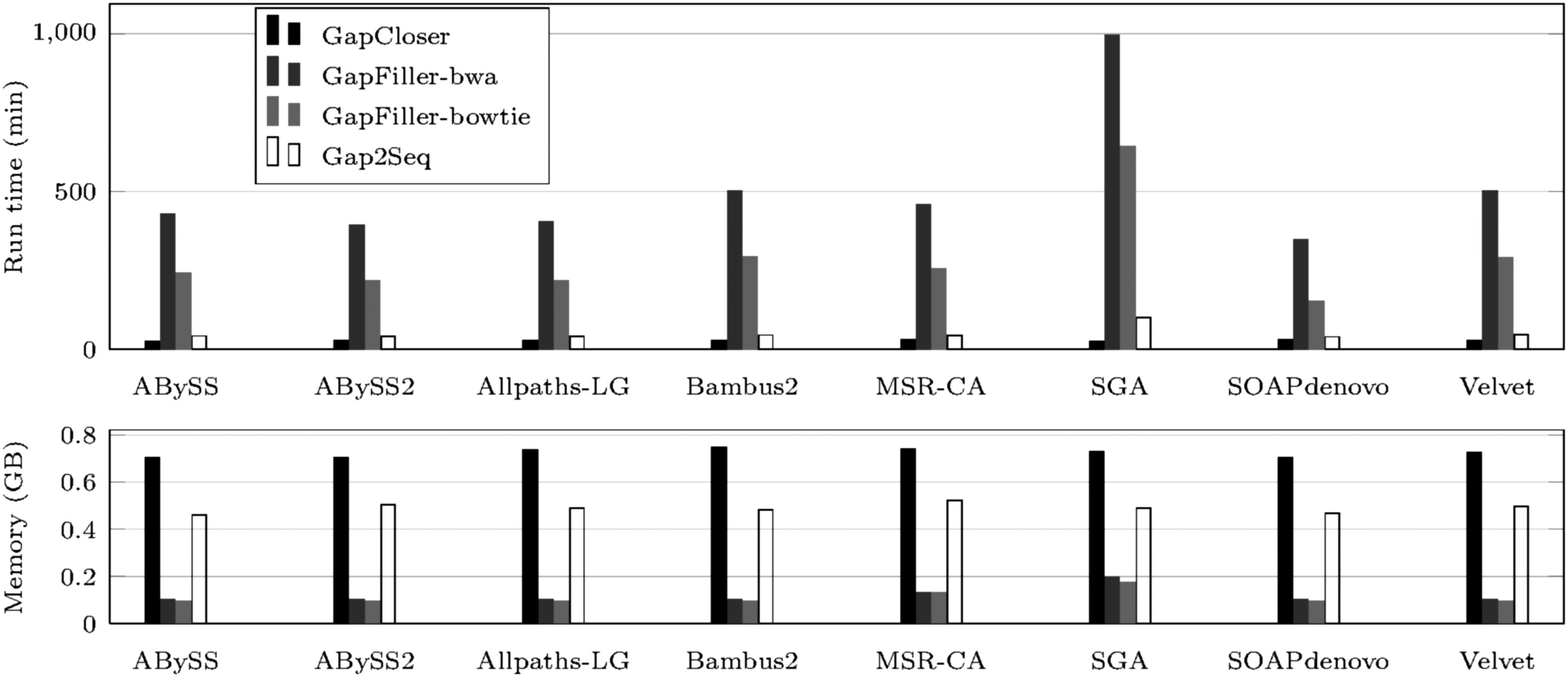
Staph: run time in minutes (above), and peak memory usage in GB (below).

FIG. 4.

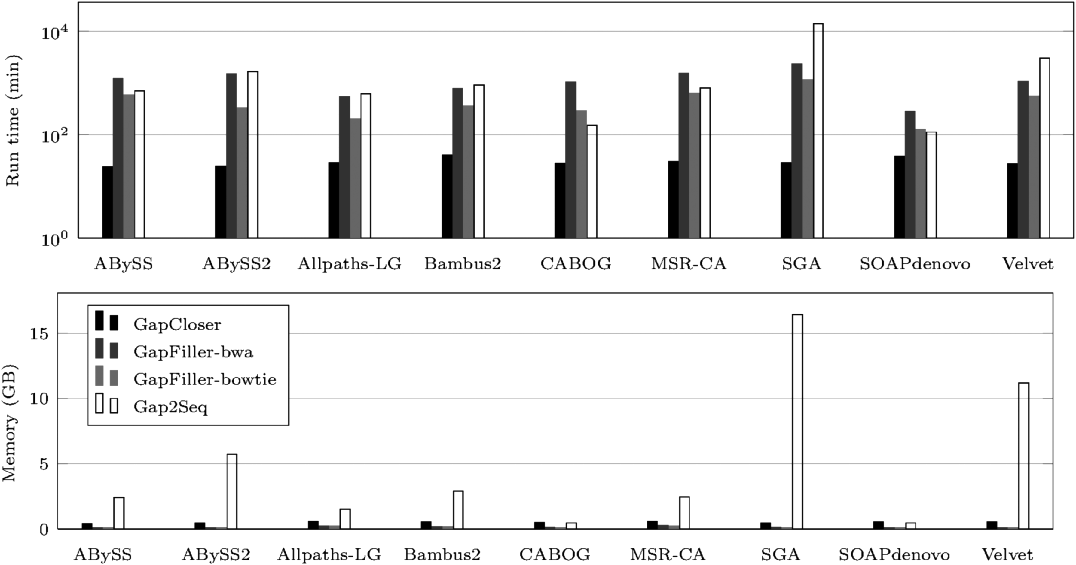
Rhodo: run time in minutes (above, logarithmic scale), and peak memory usage in GB (below).

5.2. Human chromosome 14 data set

The performance of any gap filler depends on the quality of the previous contig assembly and scaffolding phases. Accordingly, we categorized the different assemblies in the human14 GAGE data sets according to their number of misassemblies: conservative assemblies are those with at most 10 misassemblies (and NGA50 at most 10000); moderate assemblies are those with at most 100 misassemblies (and NGA50 at most 100000); and aggressive assemblies are those with more than 1000 misassemblies.

Tables 5 –7 present the performance of the gap fillers on the GAGE human14 data sets. As a general comment, we observe that the resulting erroneous sequence after filling the gaps with Gap2Seq is always the smallest, or close to the smallest, independent of the quality of the original assembly. This is most clearly seen on the conservative and moderate assemblies, where Gap2Seq exhibits the best trade-off between resulting erroneous length and filled gap length. While on the aggressive assemblies GapCloser performs the best with respect to most of the metrics, there is no clear best tool in the other two assembly categories. For example, GapFiller-bwa appears to be the best on the CABOG assembly, and GapFiller-bwa and Gap2Seq appear to be the best on the ABySS assembly.

Table 5.

Human14, Conservative Assemblies

Tool	Original	GapCloser	GapFiller-bowtie	GapFiller-bwa	Gap2Seq
ABySS
Misassemblies	3	+133.3%	+33.3%	+0%	+100%
Erroneous length	190458	+18.2%	+7.6%	+6.1%	−9.4%
Unaligned length	262068	−16.6%	−28.9%	−34.2%	−8.4%
NGA50	1320	+1.0%	+0.5%	+0.7%	+1.3%
Number of gaps	1061	−5.9%	−28.9%	−32.5%	−33.4%
Total gap length	585628	−24.5%	−23.4%	−27.6%	−25.5%
SGA
Misassemblies	8	+375%	+37.5%	+112.5%	+287.5%
Erroneous length	1580489	+21.1%	−18.4%	−14.6%	−24.6%
Unaligned length	1160159	−83.9%	−82.8%	−86.5%	−38.6%
NGA50	2644	+244.2%	+206.6%	+238.0%	+149.1%
Number of gaps	21459	−56.7%	−46.3%	−49.9%	−51.5%
Total gap length	12840408	−53.5%	−50.0%	−55.4%	−30.2%
TOTAL
Misassemblies	11	+309.1%	+36.4%	+81.8%	+236.4%
Erroneous length	1770947	+20.8%	−15.6%	−12.3%	−23.0%
Unaligned length	1422227	−71.5%	−72.8%	−76.9%	−33.0%
NGA50	3964	+163.2%	+138.0%	+159.0%	+99.9%
Number of gaps	22520	−54.3%	−45.5%	−49.1%	−50.7%
Total gap length	13426036	−52.2%	−48.8%	−54.2%	−30.0%

The formatting is the same as in Table 3.

Table 6.

Human14, Moderate Assemblies

Tool	Original	GapCloser	GapFiller-bowtie	GapFiller-bwa	Gap2Seq
ABySS2
Misassemblies	99	+18.2%	+2.0%	+3.0%	+5.1%
Erroneous length	555099	+15.9%	+1.5%	+3.3%	+3.5%
Unaligned length	157759	−21.4%	−28.8%	−36.4%	−15.4%
NGA50	11869	+4.1%	+1.5%	+3.1%	+2.4%
Number of gaps	2820	−14.5%	−29.5%	−38.5%	−23.9%
Total gap length	949137	−34.9%	−10.6%	−25.3%	−36.8%
Allpaths-LG
Misassemblies	95	−6.3%	+5.3%	+10.5%	+14.7%
Erroneous length	667229	+34.5%	−0.6%	+6.6%	−3.0%
Unaligned length	36941	−14.3%	−11.1%	−11.5%	+26.8%
NGA50	34534	+48.3%	+20.7%	+22.5%	+23.3%
Number of gaps	4307	−35.1%	−19.3%	−20.6%	−29.8%
Total gap length	3227193	−37.9%	−16.0%	−17.3%	−16.0%
CABOG
Misassemblies	91	+16.5%	+7.7%	+5.5%	+7.7%
Erroneous length	615239	+19.0%	−2.2%	−0.2%	−3.5%
Unaligned length	2506	+0%	+0%	+0%	+0%
NGA50	46665	+16.2%	+58.8%	+64.7%	+8.9%
Number of gaps	3043	−18.9%	−46.5%	−51.9%	−13.8%
Total gap length	231078	−50.3%	−34.9%	−42.0%	−22.6%
TOTAL
Misassemblies	285	+9.5%	+4.9%	+6.3%	+9.1%
Erroneous length	1837567	+23.7%	−0.5%	+3.4%	−1.2%
Unaligned length	197206	−19.8%	−25.1%	−31.3%	−7.3%
NGA50	93068	+26.6%	+37.3%	+41.2%	+13.4%
Number of gaps	10170	−24.6%	−30.3%	−34.9%	−23.4%
Total gap length	4407408	−37.9%	−15.9%	−20.3%	−20.9%

The formatting is the same as in Table 3.

Table 7.

Human14, Aggressive Assemblies

Tool	Original	GapCloser	GapFiller-bowtie	GapFiller-bwa	Gap2Seq
Bambus2
Misassemblies	1584	+3.1%	+2.3%	+4.4%	+2.1%
Erroneous length	11114542	−9.6%	−0.2%	+0.6%	−0.6%
Unaligned length	161358	−42.7%	−35.8%	−37.8%	+2.5%
NGA50	3045	+34.8%	+12.0%	+16.8%	+1.8%
Number of gaps	11809	−16.4%	−2.3%	−2.4%	−6.6%
Total gap length	10370362	−45.6%	−18.9%	−27.1%	−4.6%
MSR-CA
Misassemblies	1110	+14.5%	+9.9%	+17.6%	+6.8%
Erroneous length	5412965	+2.8%	+3.9%	+9.6%	−6.1%
Unaligned length	318421	−30.5%	−28.8%	−30.6%	−13.1%
NGA50	5704	+73.3%	+65.9%	+78.2%	+32.9%
Number of gaps	30622	−34.9%	−42.4%	−47.8%	−27.8%
Total gap length	6097928	−49.3%	−37.8%	−45.4%	−18.1%
SOAPdenovo
Misassemblies	1250	+17.1%	+3.5%	+6.1%	+11.7%
Erroneous length	8449941	−1.3%	+1.1%	+3.1%	−0.5%
Unaligned length	1306173	−28.8%	−24.4%	−27.2%	−14.1%
NGA50	6592	+17.4%	+3.6%	+4.1%	+4.0%
Number of gaps	8544	−25.2%	−4.5%	−5.2%	−18.8%
Total gap length	10255930	−21.3%	−11.3%	−15.9%	−6.3%
Velvet
Misassemblies	9308	+26.3%	+24.8%	+31.1%	+13.3%
Erroneous length	12531431	−10.4%	+32.3%	+41.1%	−0.5%
Unaligned length	23484076	−58.4%	−54.9%	−64.5%	−20.7%
NGA50	1793	+104.4%	+49.6%	+62.2%	+27.0%
Number of gaps	51567	−43.4%	−24.1%	−26.0%	−26.6%
Total gap length	63559964	−22.8%	−14.7%	−19.2%	−4.2%
TOTAL
Misassemblies	13252	+21.7%	+18.9%	+24.4%	+11.3%
Erroneous length	37508879	−6.2%	+11.6%	+16.0%	−1.3%
Unaligned length	25270028	−56.4%	−52.9%	−62.0%	−20.1%
NGA50	17134	+48.2%	+30.6%	+37.1%	+15.6%
Number of gaps	102542	−36.2%	−25.4%	−28.1%	−24.0%
Total gap length	90284184	−27.1%	−16.4%	−21.5%	−5.5%

The formatting is the same as in Table 3.

We also investigated how the length of the gap influences Gap2Seq's performance. We chose the assembly where it performs best as compared to the other gap fillers, ABySS (a conservative assembly), and an assembly where it performs worst as compared to the other gap fillers, SOAPdenovo (an aggressive assembly). We then computed the number of gaps that are filled, where there was no path whose length would fall in the required interval, and where Gap2Seq abandoned the search because it exceeded the memory limit. We plot these numbers in Figure 5. In the ABySS assembly, Gap2Seq generally fills the gaps or reports that no path exists. This is contrary to the SOAPdenovo assembly, where Gap2Seq abandons many longer gaps because it exceeds the memory limit. On the one hand, this implies that aggressive assemblies exhibit a too complex behavior to be handled by an exact algorithm running on the graph of all available reads. On the other hand, when the graph between the two flanking contigs does have a manageable size, then such an exact algorithm seems to produce indeed better results than the competing strategies.

FIG. 5.

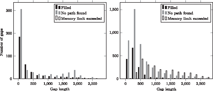
Classification of gaps as reported by Gap2Seq: filled, no path found, or memory limit exceeded. Left: human14 ABySS assembly. Right: human14 SOAPdenovo assembly. Bins of size 200 bp have been used in generating the histograms. The longest gap in the human14 SOAPdenovo assembly is 34,745 bp but the x axis has been cut at 2900 bp for easier comparison with the human14 ABySS assembly where the longest gap is 2758 bp.

Figure 6 shows the runtime and peak memory usage of the gap fillers on the human14 assemblies. GapCloser is the fastest of the methods, while GapFiller-bwa and GapFiller-bowtie are the most memory efficient ones. For Gap2Seq we see that the memory limit of 20 GB excluding the DBG is indeed reached in most cases, and except for the ABySS assembly this also translates to a long runtime.

FIG. 6.

Human14: run time in minutes (above, logarithmic scale), and peak memory usage in GB (below).

6. Conclusion

In this work we have shown that Gap2Seq has a good performance on bacterial data sets in terms of the quality of the results, with moderate computational requirements. However, such performance does not seem to scale easily to eukaryotic genomes. In fact, our experiments on moderate and aggressive assemblies of human chromosome 14 indicate that many gaps are left unfilled because of running out of resources (Fig. 5). Gap2Seq does generally have the smallest erroneous length of the resulting sequence, but since many gaps are left unfilled we cannot draw a general conclusion about the robustness of our problem formulation. Moreover, all tools exhibit varying behaviors with respect to the number of misassemblies and the number or length of the gaps closed, highlighting the difficulty of the problem in larger genomes.

For cases with many solutions to the gap-filling problem, our current traceback routine could be improved as follows. Using forward and backward computation as in hidden Markov models, one can compute for each vertex v and gap length d, the number of s-t paths of length d passing through that vertex. With one more forward sweep of the algorithm, taking the maximum of these counts, one can traceback a most robust path (see Durbin et al., 1998, Chapter 4, for an analogous computation) that involves vertices most often seen in paths of the correct length.

We note that our definition of gap filling, and hence also the algorithms presented here, are directly applicable to other related problems. For example, the method applies to finding a sequence to span the gap between the two ends of paired-end reads (Nadalin et al., 2012). However, the practical instances for this problem tend to be easier, since paired-end reads are randomly sampled from the genome, whereas in gap filling the easy regions of the genome have already been reconstructed by the contig assembler, and thus only the hard regions are left. Nevertheless, one should be more conservative in filling such gaps, as errors in this phase will be cumulated to later phases of the assembly.

Another example is in variant analysis (Pabinger et al., 2014). In projects with known reference genome, one can sequence the donor and map the reads to the reference. If there is a long insertion in the donor, paired-end read-mapping anomalies and drops in read coverage can predict where an insertion is located in the reference and how long that is. Running gap filling on the unmapped reads can be used to discover this inserted sequence.

Footnotes

Acknowledgments

This work was supported by the Academy of Finland (grants 284598 [CoECGR], 267591 to L.S., and 274977 to A.I.T.), by KTH opportunities fund (grant V-2013-019 to K.S.) and in part by the Swedish Research Council (grant 2010-4634).

Author Disclosure Statement

No competing financial interests exist.

References

Bellman

1958. On a routing problem. Q. Appl. Math., 16, 87–90.

Boetzer

, and Pirovano

2012. Toward almost closed genomes with GapFiller. Genome Biol. 13, R56.

Drezen

, Rizk

, Chikhi

, et al. 2014. GATB: Genome assembly & analysis tool box. Bioinformatics, 30, 2959–2961.

Durbin

, Eddy

S.R.

, Krogh

, et al. 1998. Biological Sequence Analysis: Probabilistic Models of Proteins and Nucleic Acids. Cambridge University Press, Cambridge, UK.

Dyer

M.E.

, Frieze

, Kannan

, et al. 1993. A mildly exponential time algorithm for approximating the number of solutions to a multidimensional knapsack problem. Combinatorics Probability Comput. 2, 271–284.

Garey

M.R.

, and Johnson

D.S.

1979. Computers and Intractability: A Guide to the Theory of NP-Completeness. W. H. Freeman & Co., New York.

Gnerre

, MacCallum

, Przybylski

, et al. 2011. High-quality draft assemblies of mammalian genomes from massively parallel sequence data. Proc. Natl. Acad. Sci. USA, 108, 1513–1518.

Gurevich

, Saveliev

, Vyahhi

, et al. 2013. QUAST: Quality assessment tool for genome assemblies. Bioinformatics, 29, 1072–1075.

Jackman

S.D.

, Raghavan

, Vandervalk

B.P.

, et al. 2015. Scaling ABySS to longer reads using spaced k-mers and Bloom filters. Poster presented at RECOMB 2015.

10.

Karp

R.M.

1972. Reducibility among combinatorial problems, 85–103. In Miller

R.E.

, and Thatcher

J.W.

, eds. Complexity of Computer Computations. Plenum Press, New York.

11.

Kurtz

, Phillippy

, Delcher

A.L.

, et al. 2004. Versatile and open software for comparing large genomes. Genome Biol. 5, R12.

12.

Langmead

, Trapnell

, Pop

, et al. 2009. Ultrafast and memory-efficient alignment of short DNA sequences to the human genome. Genome Biol. 10, R25.

13.

, and Durbin

2009. Fast and accurate short read alignment with Burrows-Wheeler transform. Bioinformatics, 25, 1754–1760.

14.

Luo

, Liu

, Xie

, et al. 2012. SOAPdenovo2: An empirically improved memory-efficient short-read de novo assembler. GigaScience, 1, 18.

15.

Nadalin

, Vezzi

, and Policriti

2012. GapFiller: A de novo assembly approach to fill the gap within paired reads. BMC Bioinform. 13, S8.

16.

Nykänen

, and Ukkonen

2002. The exact path length problem. J. Algorithms, 42, 41–53.

17.

Pabinger

, Dander

, Fischer

, et al. 2014. A survey of tools for variant analysis of next-generation genome sequencing data. Brief. Bioinform., 15, 256–278.

18.

Pevzner

P.A.

, and Tang

2001. Fragment assembly with double-barreled data. Bioinformatics, 17, S225–S233.

19.

Salmela

, Sahlin

, MäKinen

, and Tomescu

A.I.

2015. Gap2Seq. Available at www.cs.helsinki.fi/u/LmsaLmeL/Gap2Seq/. Accessed Feb. 19, 2016.

20.

Salzberg

S.L.

, Phillippy

A.M.

, Zimin

, et al. 2012. GAGE: A critical evaluation of genome assemblies and assembly algorithms. Genome Res. 22, 557–567.

21.

Simpson

J.T.

, and Durbin

2012. Efficient de novo assembly of large genomes using compressed data structures. Genome Res. 22, 549–556.

22.

Simpson

J.T.

, Wong

, Jackman

S.D.

, et al. 2009. ABySS: A parallel assembler for short read sequence data. Genome Res. 19, 1117–1123.

23.

Wetzel

, Kingsford

, and Pop

2011. Assessing the benefits of using mate-pairs to resolve repeats in de novo short-read prokaryotic assemblies. BMC Bioinform. 12, 95.