Computational Protein Design Using AND/OR Branch-and-Bound Search

Abstract

The computation of the global minimum energy conformation (GMEC) is an important and challenging topic in structure-based computational protein design. In this article, we propose a new protein design algorithm based on the AND/OR branch-and-bound (AOBB) search, a variant of the traditional branch-and-bound search algorithm, to solve this combinatorial optimization problem. By integrating with a powerful heuristic function, AOBB is able to fully exploit the graph structure of the underlying residue interaction network of a backbone template to significantly accelerate the design process. Tests on real protein data show that our new protein design algorithm is able to solve many problems that were previously unsolvable by the traditional exact search algorithms, and for the problems that can be solved with traditional provable algorithms, our new method can provide a large speedup by several orders of magnitude while still guaranteeing to find the global minimum energy conformation (GMEC) solution.

1. Introduction

In a structure-based computational protein design (SCPD) problem, we aim to find a new amino acid sequence that accommodates certain structural requirements and thus can perform desired functions by replacing several residues from a wild-type protein template. The SCPD has exhibited promising applications in numerous biological engineering situations, such as enzyme synthesis (Chen et al., 2009), drug resistance prediction (Frey et al., 2010), drug design (Gorczynski et al., 2007), and design of protein–protein interactions (Roberts et al., 2012).

The aim of SCPD is to find the global minimum energy conformation (GMEC), that is, the global optimal solution of an amino acid sequence that minimizes a defined energy function. In practice, the rigid body assumption, which anchors the backbone template, is usually applied to reduce computational complexity. In addition, possible side-chain assignments for a residue are further discretized into several known conformations, called the rotamer library. It has been proved that SCPD is NP-hard (Pierce and Winfree, 2002) even with the two aforementioned prerequisites. A number of heuristic methods have been proposed to approximate the GMEC (Street and Mayo, 1999; Kuhlman and Baker, 2000; Marvin and Hellinga, 2001). Unfortunately, these heuristic methods can be trapped into local minima and may lead to poor quality of the final solution. On the other hand, several exact and provable search algorithms that guarantee to find the GMEC solution have been proposed, such as dead-end elimination (DEE) (Desmet et al., 1992), A* search (Leach et al., 1998; Lippow and Tidor, 2007; Donald, 2011; Zhou and Zeng, 2015), tree decomposition (Xu and Berger, 2006), branch-and-bound (BnB) search (Hong and Lozano-Pérez, 2006; Traoré et al., 2013; Allouche et al., 2014), and BnB-based linear integer programming (Althaus et al., 2002; Kingsford et al., 2005).

In our protein design scheme, a set of DEE criteria (Goldstein, 1994; Gainza et al., 2012) are first applied to prune the infeasible rotamers that are provably not in the GMEC solution. After that, the AND/OR branch-and-bound (AOBB) search (Marinescu and Dechter, 2009) is used to traverse over the remaining conformational space to find the GMEC solution. Based on an advanced heuristic function, our new design algorithm can fully exploit the graph structure of the underlying residue interaction network and efficiently prune a large number of infeasible branches during the search. In addition, we propose an elegant extension of this AND/OR branch-and-bound algorithm to compute the top k solutions within a user-defined energy cutoff from the GMEC. Our tests on real protein data show that our new protein design algorithm can address many design problems that cannot be solved precisely, and for the problems that were solvable formerly, our new method can achieve a significant speedup by several orders of magnitude compared to the traditional exact search algorithms.

1.1. Related work

The A* algorithm (Leach et al., 1998; Keedy et al., 2013) was proposed to combine with DEE pruning to compute the GMEC solution. It uses a priority queue to store all the expanded states, which unfortunately may exceed the hardware memory limitation for large problems. AOBB, on the contrary, uses depth-first-search strategy that only requires linear space complexity with respect to the number of mutable residues.

The traditional BnB search algorithm (Hong and Lozano-Pérez, 2006) usually ignores the underlying topological information of the residue interaction network constructed based on the backbone template, while AOBB is designed to exploit this property.

Although the tree decomposition method (Xu and Berger, 2006) utilizes the residue interaction network, it lacks an efficient method to traverse the whole conformational space when the tree width is large and the table allocated by its dynamic programming routine may be too large to fit in memory. To fix this problem, AOBB adopts the mini-bucket heuristic to prune a large number of states to speed up the search process.

2. Methods

2.1. Overview

Under the assumptions of rigid backbone structures and discrete side-chain conformations, the structure-based computational protein design (SCPD) can be formulated as a combinatorial optimization problem that aims to find the best rotamer sequence r = (r₁, …, r_n) that minimizes the following objective function: \documentclass{aastex}\usepackage{amsbsy}\usepackage{amsfonts}\usepackage{amssymb}\usepackage{bm}\usepackage{mathrsfs}\usepackage{pifont}\usepackage{stmaryrd}\usepackage{textcomp}\usepackage{portland, xspace}\usepackage{amsmath, amsxtra}\pagestyle{empty}\DeclareMathSizes{10}{9}{7}{6}\begin{document} \begin{align*}{E_T} ( r ) = {E_0} + \mathop \sum \limits_{i = 1}^n {E_1} ( {r_i} ) + \mathop \sum \limits_{i = 1}^n \mathop \sum \limits_{j = i + 1}^n {E_2} ( {r_i} , {r_j} ) {} , \tag{1}\end{align*} \end{document}

where n stands for the number of mutable residues, E_T (r) represents the total energy of the system in which the rotamer assignment of the mutable residues is r, E₀ represents the template energy (i.e., the sum of the backbone energy and the energy among nonmutable residues), E₁(r_i) represents the self energy of rotamer r_i (i.e., the sum of intra-residue energy and the energy between r_i and nonmutable residues), and E₂(r_i, r_j) is the pairwise energy between rotamers r_i and r_j.

To find the global minimum energy conformation (GMEC), we often need to search over a huge conformational space. Our search scheme followed the popular protein design pipeline in the literature (Leach et al., 1998; Keedy et al., 2013): First, a combination of several dead-end elimination criteria (Goldstein, 1994; Gainza et al., 2012) was applied to prune the rotamers that are provably not in the optimal solution and thus reduce the magnitude of the search space. Then, a combinatorial optimization algorithm, namely the AND/OR branch-and-bound search, is used to traverse the remaining conformational space and guarantees finding the GMEC solution.

2.2. AND/OR branch-and-bound search

2.2.1. Branch-and-bound search

Suppose we try to find the global minimum value of the energy function E(r), in which r∈R and R is the conformational space of the rotamers. The BnB algorithm executes two steps recursively. The first step is called branching, in which we split the conformational space R into two or more smaller spaces, that is, R₁, R₂, …, R_m, where \documentclass{aastex}\usepackage{amsbsy}\usepackage{amsfonts}\usepackage{amssymb}\usepackage{bm}\usepackage{mathrsfs}\usepackage{pifont}\usepackage{stmaryrd}\usepackage{textcomp}\usepackage{portland, xspace}\usepackage{amsmath, amsxtra}\pagestyle{empty}\DeclareMathSizes{10}{9}{7}{6}\begin{document} $${R_1} \cup {R_2} \cup \ldots \cup {R_m} = R$$ \end{document} . If we are able to find \documentclass{aastex}\usepackage{amsbsy}\usepackage{amsfonts}\usepackage{amssymb}\usepackage{bm}\usepackage{mathrsfs}\usepackage{pifont}\usepackage{stmaryrd}\usepackage{textcomp}\usepackage{portland, xspace}\usepackage{amsmath, amsxtra}\pagestyle{empty}\DeclareMathSizes{10}{9}{7}{6}\begin{document} $${ \hat r_i} = \arg \mathop { \min } \nolimits_{r \in {R_i}} E ( r )$$ \end{document} for all \documentclass{aastex}\usepackage{amsbsy}\usepackage{amsfonts}\usepackage{amssymb}\usepackage{bm}\usepackage{mathrsfs}\usepackage{pifont}\usepackage{stmaryrd}\usepackage{textcomp}\usepackage{portland, xspace}\usepackage{amsmath, amsxtra}\pagestyle{empty}\DeclareMathSizes{10}{9}{7}{6}\begin{document} $$i \in \{ 1 , 2 , \ldots , m \} $$ \end{document} , we can compute the minimum energy conformation in the conformational space R by identifying one of \documentclass{aastex}\usepackage{amsbsy}\usepackage{amsfonts}\usepackage{amssymb}\usepackage{bm}\usepackage{mathrsfs}\usepackage{pifont}\usepackage{stmaryrd}\usepackage{textcomp}\usepackage{portland, xspace}\usepackage{amsmath, amsxtra}\pagestyle{empty}\DeclareMathSizes{10}{9}{7}{6}\begin{document} $${ \hat r_i}$$ \end{document} that has the lowest energy.

The second step of BnB is called bounding. Suppose the current lowest energy conformation is \documentclass{aastex}\usepackage{amsbsy}\usepackage{amsfonts}\usepackage{amssymb}\usepackage{bm}\usepackage{mathrsfs}\usepackage{pifont}\usepackage{stmaryrd}\usepackage{textcomp}\usepackage{portland, xspace}\usepackage{amsmath, amsxtra}\pagestyle{empty}\DeclareMathSizes{10}{9}{7}{6}\begin{document} $$\overline {r_i}$$ \end{document} . For any subspace R_j, if we can ensure that the lower bound of the energy of all conformations in R_j is greater than \documentclass{aastex}\usepackage{amsbsy}\usepackage{amsfonts}\usepackage{amssymb}\usepackage{bm}\usepackage{mathrsfs}\usepackage{pifont}\usepackage{stmaryrd}\usepackage{textcomp}\usepackage{portland, xspace}\usepackage{amsmath, amsxtra}\pagestyle{empty}\DeclareMathSizes{10}{9}{7}{6}\begin{document} $$E ( \overline {r_i} )$$ \end{document} , we can prune the whole subspace R_j safely. The lower bound of the energy of the conformations in a given space usually can be computed based on some heuristic functions. The BnB algorithm performs the branching and bounding steps recursively until the current conformational space contains only one single conformation. A more detailed introduction to branch-and-bound search can be found in appendix section 5.1.

2.2.2. Residue interaction network

Traditional BnB algorithm can hardly exploit the underlying graph structure of the residue–residue interactions. In a real design problem, some mutable residues can be relatively distant and thus the pairwise energy terms in Equation (1) between these residues are usually negligible. Based on this observation, we can construct a residue interaction network, in which each node represents a residue, and two nodes are connected by an undirected edge if and only if the distance between them is less than a threshold. Figure 1a gives an example of such a residue interaction network.

FIG. 1.

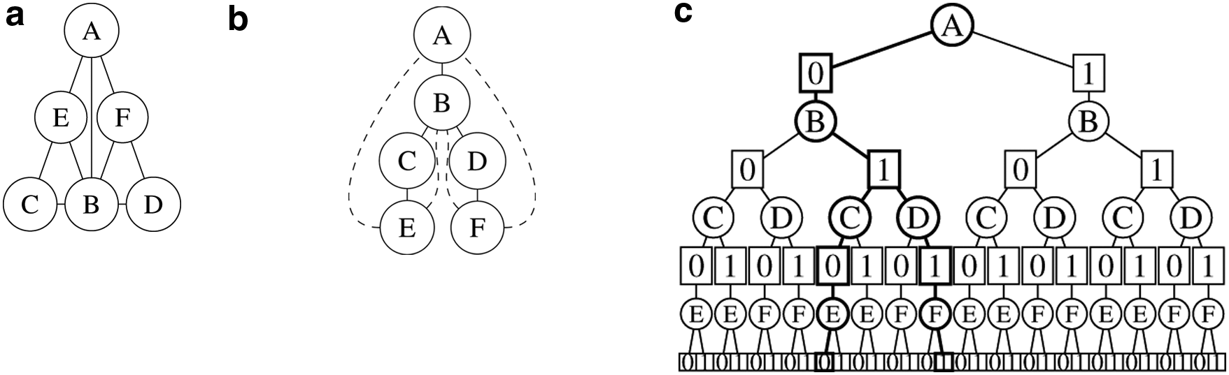
An example of constructing an AND/OR search tree. (a) An example of a residue interaction network. (b) The corresponding pseudo-tree of the residue interaction network in (a), in which dashed lines are non-tree edges. (c) The full AND/OR search tree constructed from the pseudo-tree in (b), in which circle nodes represent OR nodes and rectangle nodes represent AND nodes. An example of a solution tree for the AND/OR search tree in (c) is marked in bold.

Consider a residue interaction network that contains two connected components (i.e., two clusters of mutable residues at two distant positions). Suppose each residue has at most p rotamers and the size of each connected component is q. Then the traditional BnB search needs to visit O(p^2q) nodes in the worst case. However, from the residue interaction network, we know that two connected components are independent, which means that altering the rotamers in one connected component does not affect the pairwise energy terms in the other connected component. So we can run the BnB search for each connected component independently and then put the resulting minimum energy conformations together to form the GMEC solution, which only needs to visit O(p^q) nodes in the worst case.

The independence requirement of connected components in a residue interaction network is too strict in practice. In fact, we can partition the whole network into several independent connected components after choosing particular rotamers for some residues. For example, after fixing the rotamers for residues A and B in the example shown in Figure 1a, we can obtain two independent components CE and DF. Then we can use the aforementioned method to reduce the size of search space and then search it using branch-and-bound algorithm. This is the major motivation of AND/OR branch-and-bound (AOBB) search (Marinescu and Dechter, 2009).

2.2.3. AND/OR search space

A pseudo-tree (Freuder and Quinn, 1985) of a graph (network) is a rooted spanning tree on that graph in which every nontree edge in the graph is connected from a node to its offspring in the spanning tree. In other words, nontree edges are not allowed to connect two nodes that are located in different branches of the spanning tree. Figure 1b shows an example of a pseudo-tree constructed based on the residue interaction network in Figure 1a.

The pseudo-tree is a useful representation because for any node x in the tree, once all the side-chains of x and its ancestors are fixed, all the subtrees rooted at the children of node x are independent. In other words, altering the rotamers for the subtree rooted at a child of x does not affect the total energy of the another subtree. Thus, the size of the search space for all subtrees rooted at children of node x is proportional to the sum of the sizes of these subtrees rather than the product of their sizes as in the traditional BnB algorithm. Therefore, AOBB often has a much smaller search space compared to the traditional BnB search.

The structure of an AOBB search tree is determined by its pseudo-tree. To represent the dependency between nodes, an AOBB search tree contains two types of nodes. The first type of nodes is called OR nodes, which splits the space into several parts that cover the original space by assigning a particular rotamer to a residue. The second type of nodes is called AND nodes, which decomposes the space into several smaller spaces where the computations of total energy of residues in different branches are independent of each other. The root of an AOBB search tree is an OR node, and all the leaves are AND nodes. For each node in an AOBB search tree, its type is different from that of its parent. An example of an AOBB search tree is given in Figure 1c.

Unlike the traditional BnB search, in which a solution is represented by a single leaf node, in an AOBB search tree, a valid conformation is represented by a tree, called the solution tree. A solution tree shares the same root with the AOBB search tree. If an AND node is in the solution tree, all its OR children are also in the tree. If an OR node is in the solution tree, exactly one of its AND children is in the tree. The tree with bold lines in Figure 1c shows an example of a solution tree. To compute the best solution tree with the minimum energy when traversing the search space, we can maintain a node value v(x) to store the total energy involving the residues in the subtree rooted at x. In an AOBB search tree, v(x) can be computed as follows: \documentclass{aastex}\usepackage{amsbsy}\usepackage{amsfonts}\usepackage{amssymb}\usepackage{bm}\usepackage{mathrsfs}\usepackage{pifont}\usepackage{stmaryrd}\usepackage{textcomp}\usepackage{portland, xspace}\usepackage{amsmath, amsxtra}\pagestyle{empty}\DeclareMathSizes{10}{9}{7}{6}\begin{document} \begin{align*}v ( x ) = \begin{cases}0 , \quad \quad \quad \quad \quad \quad \quad \quad \ \ \ \ { \rm if} \ x \ { \rm is \ a \ leaf \ node}; \\ \sum_{y \in { \rm child} ( x ) } v ( y ) , \quad \quad \quad \ { \rm if} \ x \ { \rm is \ an \ internal \ AND \ node}; \\ \min_{y \in { \rm child} ( x ) } e ( y ) + v ( y ) , \ { \rm if} \ x \ { \rm is \ an \ internal \ OR \ node , }\end{cases} \tag{2}\end{align*} \end{document}

where child(x) stands for the set of children of node x and e(y) is the sum of the self energy of the rotamer represented by y and the pairwise energy between the rotamer represented by y and other rotamers represented by the ancestors of y. Then the v(·) value of the root of the whole search tree is equal to the energy of the GMEC solution. The corresponding best solution tree can be constructed using a similar method.

Algorithm 1 provides the pseudocode of the AOBB search algorithm. For simplicity, we leave out the code of constructing solution trees and only describe the procedure of computing v(·) values. For each OR node x, we use c(x) to store the pointer to the child with the best v(·) value if the subtree rooted at x has been fully explored (line 13), or the pointer to the child whose subtree is currently being visited (line 6), or a null pointer if x has not been visited (line 1).

Algorithm 1

An implementation of AND/OR branch-and-bound search

1: Initialize c(x) to null for all x	22: for all y ∈child(x) do
2: function AOBB(x)	23: v(x)←v(x) + AOBB(y)
3: if x is an OR node then	24: end for
4: v(x) ←+∞	25: end if
5: for all y ∈child(x) do	26: return v(x)
6: c(x)←y	27: end function
7: call AOBB(y)	28: function Tree-Heuristic(x)
8: if e(y) + v(y) < v(x) then	29: if x is an AND node then
9: c ₀←y	30: s ← 0
10: v(x)←e(y) + v(y)	31: for all y ∈child(x) do
11: end if	32: s ←s+ Tree-Heuristic(y)
12: end for	33: end for
13: c(x)←c ₀	34: return s
14: else if x is an AND node then	35: else
15: v(x)←0	36: if c(x) = null then
16: for all y that are x's ancestors do	37: return h(x)
17: if Tree-Heuristic(y) > v(y) then	38: end if
18: mark x as pruned	39: t ←Tree-Heuristic(c(x))
19: return +∞	40: return e(c(x))+t
20: end if	41: end if
21: end for	42: end function

The bounding step can also be performed in AOBB to prune unpromising branches. The heuristic function h(x) returns a lower bound of v(x), which is used to compute the heuristic value of an incomplete solution tree. When performing the bounding step for an AND node x, we examine all the OR ancestors' nodes of x. For any OR ancestor y, if the heuristic value for the current incomplete solution tree rooted at y (computed by Tree-Heuristic(y)) is worse than v(y) computed from another explored branch y, we can safely prune the current subtree rooted at x (lines 16–21 of Alg. 1). The function Tree-Heuristic(x) computes the heuristic value for the current incomplete solution tree rooted at x using a method similar to that of Equation (2), except that when it meets an unexplored node, it returns h(x) as a lower bound.

2.2.4. Heuristic function

The choice of the heuristic function h(x), which is a lower bound of v(x), heavily affects the performance of the AOBB algorithm. A popular heuristic function used with AOBB is called mini-bucket heuristic (Kask and Dechter, 2001), which is computed by the mini-bucket elimination algorithm (Dechter and Rish, 2003). The computation of mini-bucket heuristic can be accelerated through precomputation, so that h(x) can be computed efficiently by looking up of precomputed tables. The bound given by the mini-bucket heuristic can be further tighten by max-product linear programming (Globerson and Jaakkola, 2008) and join graph linear programming (Ihler et al., 2012).

The mini-bucket elimination is an approximation of the bucket elimination algorithm (Dechter, 1998), which is an another exact algorithm for solving the combinatorial problem with an underlying graph structure, such as protein design, based on a pseudo-tree. More specifically, the bucket elimination algorithm maintains an energy table h_x(·) for each tree node x, which stores the exact lower bound on the sum of energy involving the residues in the subtree rooted at x given the rotamer assignments of x's ancestors. For instance, h_D(r_A, r_B, r_C) in Figure 2a stores the exact lower bound of node D given the rotamer assignments of its ancestors r_A, r_B, and r_C. These energy tables can be computed in a bottom-up manner. As an example, Figure 2a shows the energy tables of the bucket elimination on a pseudo-tree of a residue interaction network, and we can compute h_C(r_A,r_B) = min_rC(E(r_B,r_C)+h_D(r_A,r_B,r_C)+h_E(r_B,r_C)), where E(r_B,r_C) represents the pairwise energy term between rotamers r_B and r_C. The h value of the tree root, h_A(), in this example, is the total energy of the GMEC. The time complexity of bucket elimination is O(n*exp(w)) (Dechter, 1998), where n is the number of the nodes and w is the tree width (Robertson and Seymour, 1986) of the graph.

FIG. 2.

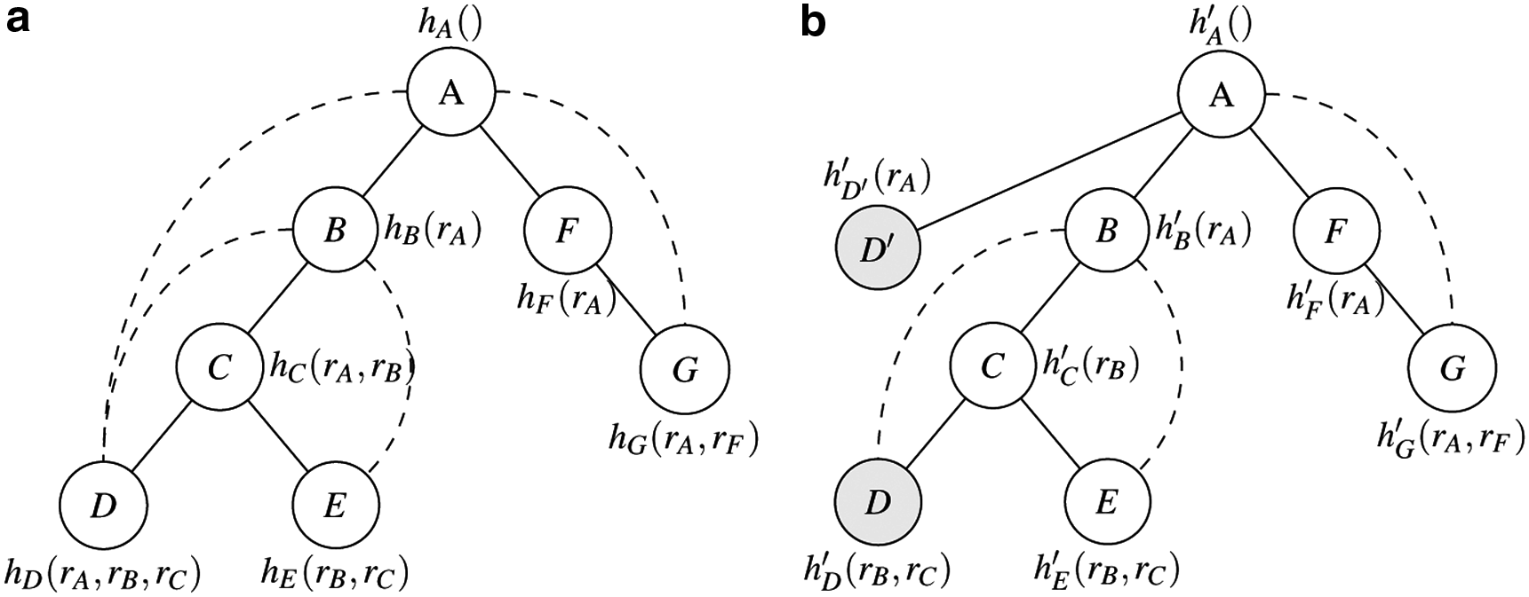
An example of mini-bucket elimination. (a) The pseudo-tree of a graph along with the resulting energy tables computed by the bucket elimination algorithm. The dashed lines represent the nontree edges in the original graph. (b) The tree generated by the mini-bucket elimination algorithm for the pseudo-tree in (a), in which the original energy table h_D(r_A, r_B, r_C) is split into two smaller tables h′_D(r_B, r_C) and h′_D′(r_A).

If the tree width of a graph is large, the energy tables may be high-dimensional and thus can be too large to compute. The mini-bucket elimination is proposed to address this problem. In particular, it splits a node with a large energy table into multiple nodes with smaller energy tables, called mini-buckets, along with the pairwise energy term represented by the new added edges to decrease the dimension of its original energy table. We use h′_x(·) to represent the new energy table for each node x computed by the mini-bucket algorithm. Figure 2b gives an example, in which h_D(r_A,r_B,r_C) is split into two smaller tables h′_D(r_B,r_C) = min _rD (E(r_D,r_B)+E(r_D,r_C)) and h′_D′(r_A) = min_rDE(r_D,r_A). Because now D and D′ can be assigned with different rotamers, the new energy tables computed by the bucket elimination on the new graph is a lower bound of the original problem. Therefore, we can use the sum of h′_x(·) on all mini-buckets of a node as the heuristic function for AOBB.

The size of an AOBB search tree is determined by the depth of its pseudo-tree, and usually the mini-bucket heuristic prefers a small tree width to generate a tight lower bound. The min-fill heuristic (Kjerulff, 1990) is often used with the mini-bucket heuristic to generate such a high-quality pseudo-tree.

2.3. Finding sub-optimal conformations

In practice, we often require the design algorithm to output at most k best conformations within a given energy cutoff Δ (Donald, 2011). In the BnB framework, this can be done easily by running the BnB search k times and removing the optimal conformations found in the preceding rounds from the search space. The task is more complicated to tackle in the AOBB because a conformation is represented by a solution tree rather than a tree node. Our solution consists of two parts:

1. In bounding steps, do not prune nodes in which the heuristic function values of the corresponding solution trees do not exceed the critical value by Δ, that is, line 17 in Algorithm 1 is changed to Tree- Heuristic(y) + Δ > v(y);

2. Keep track of the k best solution trees and their v(·) values rather than only a single solution.

For the second part, we need to extend the procedure of computing v(x), originally described in Equation (2). For each node x, we now store the k node values. Let v₁(x) be the best node value, v₂(x) be the second one, and so on. For each leaf node x, v₁(x) = 0 and \documentclass{aastex}\usepackage{amsbsy}\usepackage{amsfonts}\usepackage{amssymb}\usepackage{bm}\usepackage{mathrsfs}\usepackage{pifont}\usepackage{stmaryrd}\usepackage{textcomp}\usepackage{portland, xspace}\usepackage{amsmath, amsxtra}\pagestyle{empty}\DeclareMathSizes{10}{9}{7}{6}\begin{document} $$v_2 ( x ) = v_3 ( x ) = \cdots = v_k ( x ) = \infty$$ \end{document} . For each OR node x, we can compute \documentclass{aastex}\usepackage{amsbsy}\usepackage{amsfonts}\usepackage{amssymb}\usepackage{bm}\usepackage{mathrsfs}\usepackage{pifont}\usepackage{stmaryrd}\usepackage{textcomp}\usepackage{portland, xspace}\usepackage{amsmath, amsxtra}\pagestyle{empty}\DeclareMathSizes{10}{9}{7}{6}\begin{document} $$v_1 ( x ) \le v_2 ( x ) \le \cdots \le v_k ( x )$$ \end{document} by merging v_i(·) values of x's children using a sort routine and retaining the k smallest values.

The merge operation for AND nodes is challenging. For each AND node x, let its children be y₁, y₂, …, y_t. Our task is to find k different sequences (a₁,…,a_j,…,a_k), where a_j = (a_j₁,a_j₂,…,a_jt) and a_ji ∈{1,2,…,k}, so that \documentclass{aastex}\usepackage{amsbsy}\usepackage{amsfonts}\usepackage{amssymb}\usepackage{bm}\usepackage{mathrsfs}\usepackage{pifont}\usepackage{stmaryrd}\usepackage{textcomp}\usepackage{portland, xspace}\usepackage{amsmath, amsxtra}\pagestyle{empty}\DeclareMathSizes{10}{9}{7}{6}\begin{document} $$v_j ( x ) = \sum \nolimits_{i = 1}^{t} v_{aji} ( y_i )$$ \end{document} and \documentclass{aastex}\usepackage{amsbsy}\usepackage{amsfonts}\usepackage{amssymb}\usepackage{bm}\usepackage{mathrsfs}\usepackage{pifont}\usepackage{stmaryrd}\usepackage{textcomp}\usepackage{portland, xspace}\usepackage{amsmath, amsxtra}\pagestyle{empty}\DeclareMathSizes{10}{9}{7}{6}\begin{document} $$v_1 ( x ) \le v_2 ( x ) \le \cdots \le v_k ( x )$$ \end{document} . A brute-force method for solving this problem requires O(k^t) time complexity as it needs to enumerate all possible sequences for a₁,a₂,…,a_k, which is unacceptable because both k and t may be large in a real problem.

1: procedure Merge-And(x, y)

2: b ← (1,1,…,1)

3: Let Q be a priority queue

4: Push

\documentclass{aastex}\usepackage{amsbsy}\usepackage{amsfonts}\usepackage{amssymb}\usepackage{bm}\usepackage{mathrsfs}\usepackage{pifont}\usepackage{stmaryrd}\usepackage{textcomp}\usepackage{portland, xspace}\usepackage{amsmath, amsxtra}\pagestyle{empty}\DeclareMathSizes{10}{9}{7}{6}\begin{document} $$( Q , \left( \sum \nolimits_{i = 1}^t v_{b_j} ( y_i ) , b \right) )$$ \end{document}

5: for i ← 1 to k do

6: (s,b) ←Pop-Minimum(Q)

7: a _i ← b

\documentclass{aastex}\usepackage{amsbsy}\usepackage{amsfonts}\usepackage{amssymb}\usepackage{bm}\usepackage{mathrsfs}\usepackage{pifont}\usepackage{stmaryrd}\usepackage{textcomp}\usepackage{portland, xspace}\usepackage{amsmath, amsxtra}\pagestyle{empty}\DeclareMathSizes{10}{9}{7}{6}\begin{document} $$v_i ( x ) \rightarrow \sum \nolimits_{j = 1}^t v_{b_j} ( y_j )$$ \end{document}

9: for j ← 1 to t do

10: b′← b

11:

\documentclass{aastex}\usepackage{amsbsy}\usepackage{amsfonts}\usepackage{amssymb}\usepackage{bm}\usepackage{mathrsfs}\usepackage{pifont}\usepackage{stmaryrd}\usepackage{textcomp}\usepackage{portland, xspace}\usepackage{amsmath, amsxtra}\pagestyle{empty}\DeclareMathSizes{10}{9}{7}{6}\begin{document} $$b^{ \prime}_j \leftarrow b^{ \prime}_j + 1$$ \end{document}

12:

\documentclass{aastex}\usepackage{amsbsy}\usepackage{amsfonts}\usepackage{amssymb}\usepackage{bm}\usepackage{mathrsfs}\usepackage{pifont}\usepackage{stmaryrd}\usepackage{textcomp}\usepackage{portland, xspace}\usepackage{amsmath, amsxtra}\pagestyle{empty}\DeclareMathSizes{10}{9}{7}{6}\begin{document} $$v^{ \prime} \rightarrow \sum \nolimits_{p = 1}^t v_{b^{ \prime}_p} ( y_p )$$ \end{document}

13: Push(Q, (v′,b′))

14: end for

15: end for

16: return a

17: end procedure

A simple example and the pseudocode of our merge algorithm for an AND node are shown in Figure 3. This algorithm uses a priority queue Q, which is a data structure that supports the operations of inserting a key/value pair (i.e., element) and extracting the element with the minimum value. We first define an index sequence b = (b₁,…,b_t), where entry b_i represents the index of the chosen v(·) value in child y_i. Initially, b = (1,1,…,1) is pushed to Q. In this problem, the value of an element is the sum of v(·) values of the AND nodes' children computed using the index sequence b as the key (line 4). The initial index sequence b = (1,1,…,1) corresponds to the first sequence a₁ because we choose the best v value for each child and thus we can get the best v(·) value for their parent. Each time we extract the element with the minimum value from Q as the next best sequence (line 6). Then we push all the successors of the extracted sequence, computed by increasing only one index for each element in the sequence, into the priority queue (lines 9 to 14). We repeat these steps until all the a_i values are generated. The time complexity of this process is O(kt log(kt)), where k is the number of required suboptimal solutions and t is the number of children of an AND node. The proof of the correctness about our merge algorithm is provided in appendix section 5.2.

FIG. 3.

The merge operation for AND nodes. (a) An example where the upper part describes the problem and the lower part shows how to solve this problem using a priority queue. The numbers in small squares show the corresponding v(·) values of individual tree nodes. The shaded boxes show the element with the smallest value in each priority queue. (b) The pseudocode of the merge operation for AND nodes.

2.4. Complexity analysis

In this section, we analyze the complexity of the AOBB search algorithm and compare it with other algorithms in the literature. Because AOBB uses the depth-first-search strategy, its space complexity is O(n), where n is the total number of mutable residues. The time complexity of the AOBB algorithm is determined by the depth of its pseudo-tree, which is O(n*p^d) in the worst case, where p is the number of rotamers per residue and d is the depth of the pseudo-tree, as the size of the AOBB search tree is O(p^d), and for each tree node we need to compute Tree-Heuristic(x), whose time complexity is O(n) assuming the heuristic function h(x) can be computed in O(1) time. The following theorem gives a theoretical bound on the depth of the pseudo-tree and establishes a connection between the AOBB and tree-decomposition methods:

Theorem 2.1 (Bayardo and Miranker, 1996; Dechter and Mateescu, 2007). For any graph G = (V,E) that has a tree decomposition with tree-width ω, there exists a pseudo-tree T for G whose depth is less or equal than ω · log₂|V|.

Therefore, the worst-case complexity of AOBB is \documentclass{aastex}\usepackage{amsbsy}\usepackage{amsfonts}\usepackage{amssymb}\usepackage{bm}\usepackage{mathrsfs}\usepackage{pifont}\usepackage{stmaryrd}\usepackage{textcomp}\usepackage{portland, xspace}\usepackage{amsmath, amsxtra}\pagestyle{empty}\DeclareMathSizes{10}{9}{7}{6}\begin{document} $$O ( n*p^{ \omega \cdot \log_2n} )$$ \end{document} given the pseudo-tree with the minimum depth, where ω is the tree-width of the residue interaction network. However, this is only a theoretical bound. The problems of finding the exact tree-width and the minimum-depth pseudo-tree has both been proven to be NP-complete (Arnborg et al., 1987; Bayardo and Miranker, 1996). On the other hand, we can argue that provided the optimal tree decomposition and pseudo-tree, the time complexity of AOBB search and dynamic programming by tree decomposition is similar (the complexity of the latter is O(n*p^ω)). The superiority of AOBB search over tree decomposition is that AOBB can take advantage of a fine-tuned heuristic to prune a significant fraction of search space, and it runs in bounded memory while dynamic programming by tree decomposition can consume exponential memory space.

When computing the suboptimal solutions, AOBB applies a more complicated algorithm (section 2.3) than traditional A* search (Donald, 2011). The time complexity for AOBB to compute the suboptimal solution is O(np^dklog(kn)), where k is the number of required suboptimal solutions, p is the number of rotamers per mutable residue, d is the depth of the pseudo-tree of the residue interaction network, and n is the total number of mutable residues. Thus, for large k, computing the sub-optimal solutions in AOBB may require a longer time compared than in traditional A* search.

3. Results

We conducted two computational experiments to evaluate the performance of our new AOBB-based protein design algorithm. In the first experiment, we compared our new AOBB-based algorithm with the traditional A*-based algorithm in a core redesign problem. To make a fair comparison, in this test we did not not make any approximation in the energy matrix (i.e., the residue interaction network is fully connected) because the A*-based algorithm cannot benefit much from such approximation. In the second computational experiment, we performed the full protein design to examine the performance of our algorithm on a larger residue interaction network.

Our AOBB-based protein design algorithm was implemented based on the protein design package OSPREY (Keedy et al., 2013) and the UAI branch of the AOBB search framework daoopt (Otten and Dechter, 2012; Otten et al., 2012). For comparison, we used the DEE/A* solver provided by the OSPREY package. In addition, we included the sequential A* solver with the improved computation of heuristic functions (Zhou et al., 2014). We used an Intel Xeon E5-1620 3.6 GHz CPU in all evaluation tests.

3.1. Core redesign

Core redesign can replace the amino acids in the core of a wild-type protein to increase its thermostability (Korkegian et al., 2005). In this experiment, we tested all the 23 protein core redesign cases that failed to be solved in using the expanded rotamer library with the rigid DEE/A* in 4G memory from Gainza et al. (2012). In addition, we picked another five design problems from Gainza et al. (2012) that were solvable within the given memory using the traditional DEE/A* algorithm. To make a fair comparison between A* and AOBB search algorithm, we did not remove any edge from the fully connected residue interaction network during the AOBB search in this test.

Table 1 summarizes the comparison results between A*-based and our AOBB-based algorithms, in which OOM and OOT represents “out of memory” and “out of time,” respectively. The memory was limited to 4G, which was the same as that in (Gainza et al., 2012), and the running time was limited to 8 hours. The first 23 rows show all the cases in Gainza et al., (2012), which were formerly unsolvable by the original A* algorithm. The column labeled as “Space size” shows the size of the conformational space after DEE pruning. The columns labeled as “A* time” and “cA* time” show the running time of the A* solvers from OSPREY and Zhou et al., (2014), respectively. The running time was measured in milliseconds and did not include the initialization steps of each algorithm. The initialization time of AOBB was relatively stable for all cases and typically took 90s to compute the mini-bucket heuristic tables and an initial bound for AOBB search.

Table 1.

The Comparison Between A ^* -based and AOBB-based Algorithms on the Core Redesign Problems

PDB	Space size	No. of A^ states*	No. of AOBB states	A^ time*	cA^ time*	AOBB time
1I27	2.03e+20	OOM	29	OOM	OOM	<1
1L9L	2.37e+19	OOM	1,599,481	OOM	OOM	2,885
1LNI	2.98e+13	OOM	3	OOM	OOM	<1
1MWQ	9.28e+17	OOM	3	OOM	OOM	<1
1OAI	3.27e+21	OOM	31	OOM	OOM	<1
1PSR	1.94e+22	OOM	20,310	OOM	OOM	29
1R6J	3.45e+25	OOM	3,296,587	OOM	OOM	9,875
1T8K	6.32e+20	OOM	581,917	OOM	OOM	1,888
1TUK	1.73e+19	OOM	188,042	OOM	OOM	723
1UCR	6.69e+19	OOM	25	OOM	OOM	<1
1UCS	1.09e+20	OOM	1,118	OOM	OOM	3
1ZZK	3.44e+15	OOM	255	OOM	OOM	<1
2BT9	5.40e+21	OOM	3,643,732	OOM	OOM	9,592
2BWF	5.54e+22	OOM	517,258,245	OOM	OOM	1,467,951
2HS1	6.35e+16	OOM	100,117	OOM	OOM	161
2O9S	3.53e+17	OOM	3	OOM	OOM	<1
2R2Z	7.47e+20	OOM	3	OOM	OOM	<1
2WJ5	1.47e+20	OOM	140,412,110	OOM	OOM	728,506
3FIL	2.62e+21	OOM	3	OOM	OOM	<1
3G21	4.59e+21	OOM	197,869	OOM	OOM	441
3JTZ	6.61e+22	OOM	5,074	OOM	OOM	8
3I2Z	4.61e+20	OOM	OOT	OOM	OOM	OOT
2RH2	1.29e+22	OOM	OOT	OOM	OOM	OOT
1IQZ	7.11e+17	18,337,117	90,195	1,824,235	40,217	117
2COV	1.14e+10	43,306	3	317	21	1
3FGV	6.44e+12	3,073,965	3	59,589	5,091	0
3DNJ	5.11e+12	569,597	4,984	7,469	570	3
2FHZ	1.83e+18	14,732,913	3,972	3,475,716	70,783	13

As shown in Table 1, the AOBB algorithm can successfully find the GMEC solutions for 21 out of the 23 problems from Gainza et al.'s, (2012) data, which were formerly unsolvable by the original A* algorithm with 4G memory. Also, we find that the number of states expanded in the AOBB search was much less than that in the traditional A* search. Accordingly, for those cases solvable by both algorithms, the AOBB search consumed less time than the traditional A* search. Probably this improvement was due to the fact that the mini-bucket heuristic with MPLP and JGLP is tighter than the heuristic function used in OSPREY.

3.2. Full protein design

In the second computational experiment, we ran the full protein design to evaluate the performance of our AOBB-based protein design algorithm. In the full protein design problem, all residues of a protein are mutable, which leads to a much larger conformational space. For each residue, we picked 1-4 the most similar amino acids, according to the BLOSUM62 matrix, as the mutation candidates. For each pair of residues A and B, we added an edge (A,B) to the residue interaction network if and only if for all rotamer assignments r_A and r_B, (max_rA,rBE(r_A,r_B)-min_rA,rBE(r_A,r_B)) > λ, where threshold parameter λ was used to trade the precision of the energy with the ease of the problem. We used λ = 0.04 for all the test cases.

Table 2 shows the test results of this computational experiment. The running time was measured in milliseconds. Here we did not list the results of the traditional A*-based algorithm because we found that A*-based algorithms were unable to find the GMEC solutions for all these test cases within 4G memory. The AOBB-based search algorithm can find the GMEC solutions for all the test cases. This demonstrates the power of the AOBB search algorithm with the state-of-the-art heuristic function, which can effectively address full protein design problems.

Table 2.

The Test Results on the Full Protein Design Problem

PDB	Space size	No. of residues	No. of edges	Tree depth	No. of AOBB states	AOBB time
1I27	6.69e+45	69	968	40	3,149	11
1M1Q	2.33e+19	71	390	17	3	<1
1T8K	2.83e+43	75	1031	42	3	<1
1XMK	2.66e+48	74	1108	40	864	2
3G36	4.28e+20	47	396	22	159	<1
3JTZ	1.96e+45	71	961	44	4,354,110	17,965

4. Conclusion and Future Work

In this article, we developed a new protein design algorithm based on the new branch-and-bound search technique (i.e., AOBB) to find the global minimum energy conformation, which speeds up the search process by several orders of magnitude compared to the traditional provable algorithms. The AOBB-based algorithm accelerates the search process by using an advanced heuristic function and can fully exploit the topology of the residue interaction network while it only has linear memory consumption. The algorithm can also output suboptimal solutions by employing an elegant modification of the original search algorithm.

Currently, our algorithm is only implemented on a single machine. It is possible to further accelerate the design process by parallelizing the AOBB search on a GPU processor or a CPU cluster on a supercomputer, which will enable us to deal with large protein design problems.

5. Appendices

5.1. Introduction to traditional branch-and-bound search

Suppose we try to find the global minimum value of the energy function E(r), in which \documentclass{aastex}\usepackage{amsbsy}\usepackage{amsfonts}\usepackage{amssymb}\usepackage{bm}\usepackage{mathrsfs}\usepackage{pifont}\usepackage{stmaryrd}\usepackage{textcomp}\usepackage{portland, xspace}\usepackage{amsmath, amsxtra}\pagestyle{empty}\DeclareMathSizes{10}{9}{7}{6}\begin{document} $$r \in R$$ \end{document} and R is the conformational space of the rotamers. The BnB algorithm executes two steps recursively. The first step is called branching, in which we split the conformational space R into two or more smaller spaces, that is R₁, R₂, …, R_m, where \documentclass{aastex}\usepackage{amsbsy}\usepackage{amsfonts}\usepackage{amssymb}\usepackage{bm}\usepackage{mathrsfs}\usepackage{pifont}\usepackage{stmaryrd}\usepackage{textcomp}\usepackage{portland, xspace}\usepackage{amsmath, amsxtra}\pagestyle{empty}\DeclareMathSizes{10}{9}{7}{6}\begin{document} $${R_1} \cup {R_2} \cup \ldots \cup {R_m} = R$$ \end{document} . If we are able to find \documentclass{aastex}\usepackage{amsbsy}\usepackage{amsfonts}\usepackage{amssymb}\usepackage{bm}\usepackage{mathrsfs}\usepackage{pifont}\usepackage{stmaryrd}\usepackage{textcomp}\usepackage{portland, xspace}\usepackage{amsmath, amsxtra}\pagestyle{empty}\DeclareMathSizes{10}{9}{7}{6}\begin{document} $${ \hat r_i} = \arg \mathop { \min } \nolimits_{r \in {R_i}} E ( r )$$ \end{document} for all \documentclass{aastex}\usepackage{amsbsy}\usepackage{amsfonts}\usepackage{amssymb}\usepackage{bm}\usepackage{mathrsfs}\usepackage{pifont}\usepackage{stmaryrd}\usepackage{textcomp}\usepackage{portland, xspace}\usepackage{amsmath, amsxtra}\pagestyle{empty}\DeclareMathSizes{10}{9}{7}{6}\begin{document} $$i \in \{ 1 , 2 , \ldots , m \} $$ \end{document} , we can compute the minimum energy conformation in the conformational space R by identifying one of \documentclass{aastex}\usepackage{amsbsy}\usepackage{amsfonts}\usepackage{amssymb}\usepackage{bm}\usepackage{mathrsfs}\usepackage{pifont}\usepackage{stmaryrd}\usepackage{textcomp}\usepackage{portland, xspace}\usepackage{amsmath, amsxtra}\pagestyle{empty}\DeclareMathSizes{10}{9}{7}{6}\begin{document} $${ \hat r_i}$$ \end{document} that has the lowest energy.

The second step of BnB is called bounding. Suppose the current lowest energy conformation is \documentclass{aastex}\usepackage{amsbsy}\usepackage{amsfonts}\usepackage{amssymb}\usepackage{bm}\usepackage{mathrsfs}\usepackage{pifont}\usepackage{stmaryrd}\usepackage{textcomp}\usepackage{portland, xspace}\usepackage{amsmath, amsxtra}\pagestyle{empty}\DeclareMathSizes{10}{9}{7}{6}\begin{document} $$\overline {r_i}$$ \end{document} . For any sub-space R_j, if we can ensure that the lower bound of the energy of all conformations in R_j is greater than \documentclass{aastex}\usepackage{amsbsy}\usepackage{amsfonts}\usepackage{amssymb}\usepackage{bm}\usepackage{mathrsfs}\usepackage{pifont}\usepackage{stmaryrd}\usepackage{textcomp}\usepackage{portland, xspace}\usepackage{amsmath, amsxtra}\pagestyle{empty}\DeclareMathSizes{10}{9}{7}{6}\begin{document} $$E ( \overline {r_i} )$$ \end{document} , we do not need to further search this subspace; that is, we can prune the whole subspace R_j safely. The lower bound of the energy of the conformations in a given space usually can be computed based on some heuristic functions.

The BnB algorithm generally performs the branching step recursively until the current conformational space contains only one single conformation. The space generated from the branching step can form a BnB search tree, in which the union of subspaces represented by the children of a node covers the whole conformational space of this node. In the protein design problem, we can split a conformational space by assigning a particular rotamer in a residue. For each node in the search tree, the bounding step is applied to prune some branches and thus shorten the search time. Figure 4 shows an example of the traditional branch-and-bound (BnB) search tree.

FIG. 4.

An example of a branch-and-bound search tree, which contains three mutable residues. The first residue has three allowed rotamers while the other two only have two allowed rotamers. The coding of a conformation is given by three integers, each of which is the index of the rotamer in the corresponding residue. Each tree node represents a conformational space. For each tree node, we split its conformational space by determining a particular rotamer in a residue. The shaded nodes are pruned in the bounding steps because the lower bound of the energy values in these nodes given by the heuristic function is greater than one of the optimal conformations in its siblings. A brute-force search for the full conformational space requires the computation of twelve conformations to guarantee the GMEC solution, while BnB only needs to compute five of them.

To traverse the BnB search tree, a queue Q is often used to store the nodes to be expanded. Initially, Q only contains the node representing the whole conformational space. Also, we maintain a global variable u to store the current lowest energy value. Initially, u can be initialized to the energy of any conformation. In practice, we often use a stochastic local search algorithm to generate a local optimal conformation so that it can be used to prune more nodes at the beginning of the search process. BnB can be executed by looping the following steps until Q becomes empty:

1. Extract the conformational space R from Q;

2. If R only contains a single conformation, update u using the energy of this conformation and then restart the loop;

3. Otherwise, split R into R₁, R₂, …, R_m by fixing a particular rotamer of a residue;

4. For each i ∈{1,2,…,m}, compute the lower bound of the energy for all nodes in space R_i. If it is smaller than u, push R_i to Q.

Usually Q is implemented by a LIFO queue (i.e., stack), so that the energy of current best conformation u can be updated as early as possible to prune more branches. In this case, the BnB algorithm runs in a depth-first-search mode. Another benefit of this mode is that memory used by the BnB algorithm is only proportional to the depth of the search tree, namely the number of mutable residues in the protein design problem. On the other hand, other search strategies, such as A* search, can store an exponential number of nodes in memory in the worst case. Algorithm 2 gives the pseudocode of an implementation of the BnB search algorithm.

Algorithm 2

Traditional branch-and-bound search

1: u ←∞	▹ Initialize u to infinity.
2: procedure Branch-And-Bound(R)
3: if \|R\| = 1 then	▹ Termination condition
4: Let r be the conformation in R
5: u ←min(u,E(r))
6: return r
7: end if
8: if h(R) > u then	▹ h(·) is a heuristic function
9: return null	▹ Bounding step
10: end if
11: Split R to R₁, R₂, …, R_m by fixing a rotamer of a particular residue
12: for i ← 1,t do
13: r_i ←Branch-and-Bound(R_i)
14: end for
15: return argmin_riE(r_i)
16: end procedure

5.2. Correctness for finding suboptimal solutions

In this section, we provide the proof of Theorem 1 in the article, which states the correctness of our merge algorithm for AND nodes. We restate that theorem in Theorem B.1.

Theorem B.1. Algorithm 3 (b) guarantees the correctness of finding the k best solutions.

Proof. It is sufficient to prove that in the i-th iteration, the element with the i-th smallest value is in the priority queue. This can be proven by contradiction.

Let i be the first round that the element with the i-th value is not in the priority queue. Suppose a_i = (a_i₁,a_i₂,…,a_it). Because i≠1, there exists j ∈{1,2,…,t} such that a_ij > 1. Sequence s = (a_i₁,…,a_i,j₋₁,a_ij − 1, a_i,j₊₁,…,a_it) must have not been expended. Otherwise, according to line 13, sequence a_i will be pushed to the priority queue, which contradicts the assumption. On the other hand, because v_j(y) is monotone with respect to j, the value of sequence s is smaller than the value of sequence a_i. This means that sequence s should be expanded before sequence a_i and thus must have already been expanded, which gives the contradiction. ■

Also, we provide the implementation of the merge operation for OR nodes in Algorithm 3. The correctness of this algorithm is self-evident, so we omit its proof here.

Algorithm 3

Merge operation for OR nodes

1: procedure Merge-Or(x , y)

2: w ← (v₁(y₁) + e(y₁),…,v_k(y₁) + e(y₁),…,v_k(y_t) + e(y_t))

▹ concatenate v_i(y_j) + e(y_j) for all i and j

3: Sort(w)

4: for i ← 1 to k do

5: v_i(x) ←w_i

6: end for

7: end procedure

Footnotes

Acknowledgments

We thank Dr. Lars Otten and Prof. Alex Ihler for their support in providing their code of the daoopt AOBB solver. Funding: This work was supported in part by the National Basic Research Program of China Grant 2011CBA00300 and 2011CBA00301; the National Natural Science Foundation of China Grant 61033001, 61361136003, and 61472205; and China's Youth 1000-Talent Program.

Author Disclosure Statement

The authors declare that no competing financial interests exist.

References

Allouche

J.D.D.

, de Givry

G.K.S.

, Schiex

I.A.T.

, et al. 2014. Computational protein design as an optimization problem. Artif. Intell., 212, 59–79.

Althaus

, Kohlbacher

, Lenhof

H.-P.

, and Müller

2002. A combinatorial approach to protein docking with flexible side chains. J. Comput. Biol., 9, 597–612.

Arnborg

, Corneil

D.G.

, and Proskurowski

1987. Complexity of finding embeddings in ak-tree. SIAM J. Algebraic Discrete Methods, 8, 277–284.

Bayardo

, and Miranker

1996. A complexity analysis of space-bound learning algorithms for the constraint satisfaction problem, 298–304. In Proceedings of the National Conference on Artificial Intelligence.

Chen

C.-Y.

, Georgiev

, Anderson

A.C.

, and Donald

B.R.

2009. Computational structure-based redesign of enzyme activity. Proc. Natl. Acad. Sci. U. S. A., 106, 3764–3769.

Dechter

1998. Bucket elimination: A unifying framework for probabilistic inference, 75–104. In Learning in Graphical Models. Springer, New York.

Dechter

, and Mateescu

2007. And/or search spaces for graphical models. Artif. Intell., 171, 73–106.

Dechter

, and Rish

2003. Mini-buckets: A general scheme for bounded inference. JACM, 50, 107–153.

Desmet

, Maeyer

M.D.

, Hazes

, and Lasters

1992. The dead-end elimination theorem and its use in protein side-chain positioning. Nature, 356, 539–542.

10.

Donald

B.R.

2011. Algorithms in Structural Molecular Biology. The MIT Press, New York.

11.

Freuder

E.C.

, and Quinn

M.J.

1985. Taking advantage of stable sets of variables in constraint satisfaction problems, 1076–1078. In International Joint Conference on Artificial Intelligence, volume 85.

12.

Frey

K.M.

, Georgiev

, Donald

B.R.

, and Anderson

A.C.

2010. Predicting resistance mutations using protein design algorithms. Proc. Natl. Acad. Sci. U. S. A., 107, 13707–13712.

13.

Gainza

, Roberts

K.E.

, and Donald

B.R.

2012. Protein design using continuous rotamers. PLoS Comput. Biol., 8, e1002335.

14.

Globerson

, and Jaakkola

T.S.

2008. Fixing max-product: Convergent message passing algorithms for MAP LP-relaxations, 553–560. In Advances in Neural Information Processing Systems.

15.

Goldstein

R.F.

1994. Efficient rotamer elimination applied to protein side-chains and related spin glasses. Biophys. J., 66, 1335–1340.

16.

Gorczynski

M.J.

, Grembecka

, Zhou

, et al., 2007. Allosteric inhibition of the protein-protein interaction between the leukemia-associated proteins Runx1 and CBFb. Chem. Biol. 14, 1186–1197.

17.

Hong

E.-J.

, and Lozano-Pérez

2006. Protein side-chain placement through MAP estimation and problem-size reduction, 219–230. In Algorithms in Bioinformatics. Springer, New York.

18.

Ihler

A.T.

, Flerova

, Dechter

, and Otten

2012. Join-graph based cost-shifting schemes. arXiv preprint arXiv:1210.4878.

19.

Kask

, and Dechter

2001. A general scheme for automatic generation of search heuristics from specification dependencies. Artif. Intell., 129, 91–131.

20.

Keedy

D.A.

, Chen

C.-Y.

, Rezam

, and Andersonl

A.C.

2013. OSPREY: Protein design with ensembles, flexibility, and provable algorithms. Methods Protein Des. 523, 87–107.

21.

Kingsford

C.L.

, Chazelle

, and Singh

2005. Solving and analyzing side-chain positioning problems using linear and integer programming. Bioinformatics, 21, 1028–1039.

22.

Kjerulff

1990. Triangulation of graphs—algorithms giving small total state space. Technical report.

23.

Korkegian

, Black

M.E.

, Baker

, and Stoddard

B.L.

2005. Computational thermostabilization of an enzyme. Science, 308, 857–860.

24.

Kuhlman

, and Baker

2000. Native protein sequences are close to optimal for their structures. Proc. Natl. Acad. Sci. U. S. A., 97, 10383–10388.

25.

Leach

A.R.

, Lemon

A.P.

, et al. 1998. Exploring the conformational space of protein side chains using dead-end elimination and the A* algorithm. Proteins Struct. Funct. Genet., 33, 227–239.

26.

Lippow

S.M.

, and Tidor

2007. Progress in computational protein design. Curr. Opin. Biotechnol., 18, 305–311.

27.

Marinescu

, and Dechter

2009. AND/OR branch-and-bound search for combinatorial optimization in graphical models. Artif. Intell., 173, 1457–1491.

28.

Marvin

J.S.

, and Hellinga

H.W.

2001. Conversion of a maltose receptor into a zinc biosensor by computational design. Proc. Natl. Acad. Sci. U. S. A., 98, 4955–4960.

29.

Otten

, and Dechter

2012. Anytime and/or depth-first search for combinatorial optimization. AI Commun., 25, 211–227.

30.

Otten

, Ihler

, Kask

, and Dechter

2012. Winning the PASCAL 2011 MAP challenge with enhanced AND/OR branch-and-bound. In DISCML.

31.

Pierce

N.A.

, and Winfree

2002. Protein design is NP-hard. Protein Eng., 15, 779–782.

32.

Roberts

K.E.

, Cushing

P.R.

, Boisguerin

, et al. 2012. Computational design of a PDZ domain peptide inhibitor that rescues CFTR activity. PLoS Comput. Biol., 8, e1002477.

33.

Robertson

, and Seymour

P.D.

1986. Algorithmic aspects of tree-width. J. Algorithms, 7, 309–322.

34.

Street

A.G.

, and Mayo

S.L.

1999. Computational protein design. Structure, 7, R105–R109.

35.

Traoré

, Allouche

, André

, et al. 2013. A new framework for computational protein design through cost function network optimization. Bioinformatics, 29, 2129–2136.

36.

, and Berger

2006. Fast and accurate algorithms for protein side-chain packing. JACM, 53, 533–557.

37.

Zhou

, and Zeng

2015. Massively parallel A* search on a GPU. In Proceedings of the National Conference on Artificial Intelligence.

38.

Zhou

, Xu

, Donald

B.R.

, and Zeng

2014. An efficient parallel algorithm for accelerating computational protein design. Bioinformatics, 30, i255–i263.