Statistically Consistent k -mer Methods for Phylogenetic Tree Reconstruction

1. Introduction

The first step in most approaches for inference of a phylogenetic tree from sequence data is to construct an alignment of the sequences intended to identify orthologous sites. When many sequences are considered at once, a full search over all possible sequence alignments is infeasible, so most algorithms reduce the range of possible alignments considered by constructing multiple alignments on subcollections of the sequences and then merging these together, using heuristic, rather than model-based, schemes. Deciding which subcollections of the sequences to align follows a guide tree, a rough tree approximating the evolutionary histories of all the sequences. This means that sequence alignment and phylogenetic tree construction are circularly entangled: finding a tree depends on knowing a multiple sequence alignment and obtaining a sequence alignment requires knowing a tree.

To get around this chicken-and-egg problem of alignment and phylogeny, several methods have been proposed. The most theoretically appealing methods are simultaneous alignment and phylogeny algorithms built upon statistical models of insertion and deletions (indels) of bases, as well as base substitutions (Thorne et al., 1991, 1992). Unfortunately, such methods are computationally intensive and do not scale well for large phylogenies. Alternatively, methods have been developed that iteratively compute alignments and phylogenies many times, using the output from one procedure as the input to the next (Liu et al., 2009, 2012). These last investigations underscored that poor alignments can be a significant source of error in trees and that better guide trees can lead to better tree inference.

If one is interested primarily in the phylogeny, an alternate strategy is to develop methods for inferring trees that do not require having a sequence alignment in hand. Current fully alignment-free phylogenetic methods were not developed with stochastic models of sequence evolution in mind and are not widely accepted in the phylogenetics community. However, the construction of initial guide trees for producing alignments generally follows an alignment-free approach. For example, MUSCLE (Edgar, 2004a,b) uses k-mer distances with unweighted pair group method with arithmetic mean (UPGMA) or Neighbor Joining to produce guide trees, whereas Clustal Omega (Sievers et al., 2011) uses a low-dimensional geometric embedding based on k-mers (Blackshields et al., 2010) and k-means or UPGMA as a clustering algorithm. Thus, even though tree inference is typically performed with model-based statistical methods, the initial step is built on heuristic ideas, with no evolutionary model in use.

As exemplified by these alignment algorithms, most common alignment-free methods are based on \documentclass{aastex}\usepackage{amsbsy}\usepackage{amsfonts}\usepackage{amssymb}\usepackage{bm}\usepackage{mathrsfs}\usepackage{pifont}\usepackage{stmaryrd}\usepackage{textcomp}\usepackage{portland, xspace}\usepackage{amsmath, amsxtra}\pagestyle{empty}\DeclareMathSizes{10}{9}{7}{6}\begin{document} $$k$$ \end{document} -mers, contiguous subsequences of length \documentclass{aastex}\usepackage{amsbsy}\usepackage{amsfonts}\usepackage{amssymb}\usepackage{bm}\usepackage{mathrsfs}\usepackage{pifont}\usepackage{stmaryrd}\usepackage{textcomp}\usepackage{portland, xspace}\usepackage{amsmath, amsxtra}\pagestyle{empty}\DeclareMathSizes{10}{9}{7}{6}\begin{document} $$k$$ \end{document} . To a sequence of length \documentclass{aastex}\usepackage{amsbsy}\usepackage{amsfonts}\usepackage{amssymb}\usepackage{bm}\usepackage{mathrsfs}\usepackage{pifont}\usepackage{stmaryrd}\usepackage{textcomp}\usepackage{portland, xspace}\usepackage{amsmath, amsxtra}\pagestyle{empty}\DeclareMathSizes{10}{9}{7}{6}\begin{document} $$n$$ \end{document} for any natural number \documentclass{aastex}\usepackage{amsbsy}\usepackage{amsfonts}\usepackage{amssymb}\usepackage{bm}\usepackage{mathrsfs}\usepackage{pifont}\usepackage{stmaryrd}\usepackage{textcomp}\usepackage{portland, xspace}\usepackage{amsmath, amsxtra}\pagestyle{empty}\DeclareMathSizes{10}{9}{7}{6}\begin{document} $$k \le n$$ \end{document} , we associate the vector of counts of its distinct \documentclass{aastex}\usepackage{amsbsy}\usepackage{amsfonts}\usepackage{amssymb}\usepackage{bm}\usepackage{mathrsfs}\usepackage{pifont}\usepackage{stmaryrd}\usepackage{textcomp}\usepackage{portland, xspace}\usepackage{amsmath, amsxtra}\pagestyle{empty}\DeclareMathSizes{10}{9}{7}{6}\begin{document} $$k$$ \end{document} -mers. For a DNA sequence, the \documentclass{aastex}\usepackage{amsbsy}\usepackage{amsfonts}\usepackage{amssymb}\usepackage{bm}\usepackage{mathrsfs}\usepackage{pifont}\usepackage{stmaryrd}\usepackage{textcomp}\usepackage{portland, xspace}\usepackage{amsmath, amsxtra}\pagestyle{empty}\DeclareMathSizes{10}{9}{7}{6}\begin{document} $$k$$ \end{document} -mer count vector has \documentclass{aastex}\usepackage{amsbsy}\usepackage{amsfonts}\usepackage{amssymb}\usepackage{bm}\usepackage{mathrsfs}\usepackage{pifont}\usepackage{stmaryrd}\usepackage{textcomp}\usepackage{portland, xspace}\usepackage{amsmath, amsxtra}\pagestyle{empty}\DeclareMathSizes{10}{9}{7}{6}\begin{document} $${4^k}$$ \end{document} entries and sums to \documentclass{aastex}\usepackage{amsbsy}\usepackage{amsfonts}\usepackage{amssymb}\usepackage{bm}\usepackage{mathrsfs}\usepackage{pifont}\usepackage{stmaryrd}\usepackage{textcomp}\usepackage{portland, xspace}\usepackage{amsmath, amsxtra}\pagestyle{empty}\DeclareMathSizes{10}{9}{7}{6}\begin{document} $$n - k + 1$$ \end{document} . The distance between two sequences might be calculated by measuring the (squared Euclidean) distance between their (suitably normalized) \documentclass{aastex}\usepackage{amsbsy}\usepackage{amsfonts}\usepackage{amssymb}\usepackage{bm}\usepackage{mathrsfs}\usepackage{pifont}\usepackage{stmaryrd}\usepackage{textcomp}\usepackage{portland, xspace}\usepackage{amsmath, amsxtra}\pagestyle{empty}\DeclareMathSizes{10}{9}{7}{6}\begin{document} $$k$$ \end{document} -mer count vectors. In this way, one obtains pairwise distances between all sequences and can apply a standard distance-based method (e.g., Neighbor Joining [NJ]) to construct a phylogenetic tree.

Such k-mer methods are sometimes described as nonparametric, in that they do not depend on any underlying statistical model describing the generation of the sequences. For phylogenetic purposes, where an evolutionary model will be assumed in later stages of an analysis, it is hard to view this as desirable. As we will show in Section 3, if we do assume that data are produced according to a standard probabilistic model of sequence evolution, then a naive k-mer method is statistically inconsistent. That is, over a rather large range of metric trees, it will not recover the correct tree from sequence data, even with arbitrarily long sequences. The statistical inconsistency of such a k-mer method is similar to the ones seen for parsimony in the Felsenstein zone (Felsenstein, 1978).

Our main result, presented in Section 2, is the derivation of a statistically consistent model-based k-mer distance under standard phylogenetic models with no indel process. It would, of course, be preferable to work with a model including indels as only in that situation is an alignment-free method of real value. At this time, however, we are only able to offer a reasonable heuristic extension of our method for sequences evolving with a mild indel process. This appears in Section 5. We view this as only a first step toward developing rigorously justified model-based k-mer methods for indel models; solid theoretical development of such methods is a project for the future.

Section 4 presents more detailed results on identifiability of model parameters from k-mer count vectors. While one of these plays a role in establishing the results of Section 2, they are of interest in their own right. Technical proofs for Sections 2 and 4 are deferred to Sections 8 and 9.

In Section 6, we report results from simulation studies on sequence data generated from models with and without an indel process, comparing k-mer methods with and without the model-based corrections. As expected, the k-mer methods with the model-based corrections outperform both the uncorrected k-mer methods and a more traditional distance method based on first computing pairwise alignments of sequences. The simulation studies also illustrate the statistical consistency of the model-based methods and the inconsistency of the standard k-mer method.

2. k-mer Formulas for indel-free sequences

In this section, we present formulas for model-based corrections to distances based on k-mer frequency counts. Technical proofs appear in Section 8. Our main result, Theorem 2.1, is quite general, applying to arbitrary pairwise distributions that are at stationarity. We use this result to derive corrected distance calculations for the Jukes–Cantor model and the Kimura two- and three-parameter models. These corrections yield statistically consistent estimates of evolutionary times between extant taxa. Coupled with a statistically consistent method for constructing a tree from distances [e.g., NJ (Saitou and Nei, 1987)], this produces a statistically consistent method for reconstructing phylogenetic trees from k-mer counts.

Let \documentclass{aastex}\usepackage{amsbsy}\usepackage{amsfonts}\usepackage{amssymb}\usepackage{bm}\usepackage{mathrsfs}\usepackage{pifont}\usepackage{stmaryrd}\usepackage{textcomp}\usepackage{portland, xspace}\usepackage{amsmath, amsxtra}\pagestyle{empty}\DeclareMathSizes{10}{9}{7}{6}\begin{document} $$S$$ \end{document} be a sequence on an \documentclass{aastex}\usepackage{amsbsy}\usepackage{amsfonts}\usepackage{amssymb}\usepackage{bm}\usepackage{mathrsfs}\usepackage{pifont}\usepackage{stmaryrd}\usepackage{textcomp}\usepackage{portland, xspace}\usepackage{amsmath, amsxtra}\pagestyle{empty}\DeclareMathSizes{10}{9}{7}{6}\begin{document} $$L$$ \end{document} -letter alphabet, \documentclass{aastex}\usepackage{amsbsy}\usepackage{amsfonts}\usepackage{amssymb}\usepackage{bm}\usepackage{mathrsfs}\usepackage{pifont}\usepackage{stmaryrd}\usepackage{textcomp}\usepackage{portland, xspace}\usepackage{amsmath, amsxtra}\pagestyle{empty}\DeclareMathSizes{10}{9}{7}{6}\begin{document} $$[ L ] : = \{ 1 , 2 , \ldots , L \} $$ \end{document} . For a natural number \documentclass{aastex}\usepackage{amsbsy}\usepackage{amsfonts}\usepackage{amssymb}\usepackage{bm}\usepackage{mathrsfs}\usepackage{pifont}\usepackage{stmaryrd}\usepackage{textcomp}\usepackage{portland, xspace}\usepackage{amsmath, amsxtra}\pagestyle{empty}\DeclareMathSizes{10}{9}{7}{6}\begin{document} $$k$$ \end{document} , let \documentclass{aastex}\usepackage{amsbsy}\usepackage{amsfonts}\usepackage{amssymb}\usepackage{bm}\usepackage{mathrsfs}\usepackage{pifont}\usepackage{stmaryrd}\usepackage{textcomp}\usepackage{portland, xspace}\usepackage{amsmath, amsxtra}\pagestyle{empty}\DeclareMathSizes{10}{9}{7}{6}\begin{document} $$X$$ \end{document} denote the vector of \documentclass{aastex}\usepackage{amsbsy}\usepackage{amsfonts}\usepackage{amssymb}\usepackage{bm}\usepackage{mathrsfs}\usepackage{pifont}\usepackage{stmaryrd}\usepackage{textcomp}\usepackage{portland, xspace}\usepackage{amsmath, amsxtra}\pagestyle{empty}\DeclareMathSizes{10}{9}{7}{6}\begin{document} $$k$$ \end{document} -mer counts extracted from \documentclass{aastex}\usepackage{amsbsy}\usepackage{amsfonts}\usepackage{amssymb}\usepackage{bm}\usepackage{mathrsfs}\usepackage{pifont}\usepackage{stmaryrd}\usepackage{textcomp}\usepackage{portland, xspace}\usepackage{amsmath, amsxtra}\pagestyle{empty}\DeclareMathSizes{10}{9}{7}{6}\begin{document} $$S$$ \end{document} . That is, for each \documentclass{aastex}\usepackage{amsbsy}\usepackage{amsfonts}\usepackage{amssymb}\usepackage{bm}\usepackage{mathrsfs}\usepackage{pifont}\usepackage{stmaryrd}\usepackage{textcomp}\usepackage{portland, xspace}\usepackage{amsmath, amsxtra}\pagestyle{empty}\DeclareMathSizes{10}{9}{7}{6}\begin{document} $$W = {w_1}{w_2} \ldots {w_k} \in { [ L ] ^k}$$ \end{document} , the coordinate \documentclass{aastex}\usepackage{amsbsy}\usepackage{amsfonts}\usepackage{amssymb}\usepackage{bm}\usepackage{mathrsfs}\usepackage{pifont}\usepackage{stmaryrd}\usepackage{textcomp}\usepackage{portland, xspace}\usepackage{amsmath, amsxtra}\pagestyle{empty}\DeclareMathSizes{10}{9}{7}{6}\begin{document} $${X^W}$$ \end{document} records the number of times that \documentclass{aastex}\usepackage{amsbsy}\usepackage{amsfonts}\usepackage{amssymb}\usepackage{bm}\usepackage{mathrsfs}\usepackage{pifont}\usepackage{stmaryrd}\usepackage{textcomp}\usepackage{portland, xspace}\usepackage{amsmath, amsxtra}\pagestyle{empty}\DeclareMathSizes{10}{9}{7}{6}\begin{document} $$W$$ \end{document} occurs as a contiguous substring in \documentclass{aastex}\usepackage{amsbsy}\usepackage{amsfonts}\usepackage{amssymb}\usepackage{bm}\usepackage{mathrsfs}\usepackage{pifont}\usepackage{stmaryrd}\usepackage{textcomp}\usepackage{portland, xspace}\usepackage{amsmath, amsxtra}\pagestyle{empty}\DeclareMathSizes{10}{9}{7}{6}\begin{document} $$S$$ \end{document} . A standard \documentclass{aastex}\usepackage{amsbsy}\usepackage{amsfonts}\usepackage{amssymb}\usepackage{bm}\usepackage{mathrsfs}\usepackage{pifont}\usepackage{stmaryrd}\usepackage{textcomp}\usepackage{portland, xspace}\usepackage{amsmath, amsxtra}\pagestyle{empty}\DeclareMathSizes{10}{9}{7}{6}\begin{document} $$k$$ \end{document} -mer method computes a distance between two sequences, \documentclass{aastex}\usepackage{amsbsy}\usepackage{amsfonts}\usepackage{amssymb}\usepackage{bm}\usepackage{mathrsfs}\usepackage{pifont}\usepackage{stmaryrd}\usepackage{textcomp}\usepackage{portland, xspace}\usepackage{amsmath, amsxtra}\pagestyle{empty}\DeclareMathSizes{10}{9}{7}{6}\begin{document} $${S_1}$$ \end{document} and \documentclass{aastex}\usepackage{amsbsy}\usepackage{amsfonts}\usepackage{amssymb}\usepackage{bm}\usepackage{mathrsfs}\usepackage{pifont}\usepackage{stmaryrd}\usepackage{textcomp}\usepackage{portland, xspace}\usepackage{amsmath, amsxtra}\pagestyle{empty}\DeclareMathSizes{10}{9}{7}{6}\begin{document} $${S_2}$$ \end{document} , of lengths, \documentclass{aastex}\usepackage{amsbsy}\usepackage{amsfonts}\usepackage{amssymb}\usepackage{bm}\usepackage{mathrsfs}\usepackage{pifont}\usepackage{stmaryrd}\usepackage{textcomp}\usepackage{portland, xspace}\usepackage{amsmath, amsxtra}\pagestyle{empty}\DeclareMathSizes{10}{9}{7}{6}\begin{document} $${n_1}$$ \end{document} and \documentclass{aastex}\usepackage{amsbsy}\usepackage{amsfonts}\usepackage{amssymb}\usepackage{bm}\usepackage{mathrsfs}\usepackage{pifont}\usepackage{stmaryrd}\usepackage{textcomp}\usepackage{portland, xspace}\usepackage{amsmath, amsxtra}\pagestyle{empty}\DeclareMathSizes{10}{9}{7}{6}\begin{document} $${n_2}$$ \end{document} , by first computing their respective \documentclass{aastex}\usepackage{amsbsy}\usepackage{amsfonts}\usepackage{amssymb}\usepackage{bm}\usepackage{mathrsfs}\usepackage{pifont}\usepackage{stmaryrd}\usepackage{textcomp}\usepackage{portland, xspace}\usepackage{amsmath, amsxtra}\pagestyle{empty}\DeclareMathSizes{10}{9}{7}{6}\begin{document} $$k$$ \end{document} -mer vectors, \documentclass{aastex}\usepackage{amsbsy}\usepackage{amsfonts}\usepackage{amssymb}\usepackage{bm}\usepackage{mathrsfs}\usepackage{pifont}\usepackage{stmaryrd}\usepackage{textcomp}\usepackage{portland, xspace}\usepackage{amsmath, amsxtra}\pagestyle{empty}\DeclareMathSizes{10}{9}{7}{6}\begin{document} $${X_1}$$ \end{document} and \documentclass{aastex}\usepackage{amsbsy}\usepackage{amsfonts}\usepackage{amssymb}\usepackage{bm}\usepackage{mathrsfs}\usepackage{pifont}\usepackage{stmaryrd}\usepackage{textcomp}\usepackage{portland, xspace}\usepackage{amsmath, amsxtra}\pagestyle{empty}\DeclareMathSizes{10}{9}{7}{6}\begin{document} $${X_2}$$ \end{document} , and then computing the squared Euclidean distance \documentclass{aastex}\usepackage{amsbsy}\usepackage{amsfonts}\usepackage{amssymb}\usepackage{bm}\usepackage{mathrsfs}\usepackage{pifont}\usepackage{stmaryrd}\usepackage{textcomp}\usepackage{portland, xspace}\usepackage{amsmath, amsxtra}\pagestyle{empty}\DeclareMathSizes{10}{9}{7}{6}\begin{document} \begin{align*} \parallel {X_1} - {X_2} \parallel _2^2 = \sum \limits_{W \in {{ [ L ] }^k}} { \left( {X_1^W - X_2^W} \right) ^2}. \end{align*} \end{document}

Consider two sequences descended from a common ancestor while undergoing a base substitution process described by standard phylogenetic modeling assumptions. More specifically, we may assume one of the sequences, \documentclass{aastex}\usepackage{amsbsy}\usepackage{amsfonts}\usepackage{amssymb}\usepackage{bm}\usepackage{mathrsfs}\usepackage{pifont}\usepackage{stmaryrd}\usepackage{textcomp}\usepackage{portland, xspace}\usepackage{amsmath, amsxtra}\pagestyle{empty}\DeclareMathSizes{10}{9}{7}{6}\begin{document} $${S_1}$$ \end{document} , is ancestral to the other, \documentclass{aastex}\usepackage{amsbsy}\usepackage{amsfonts}\usepackage{amssymb}\usepackage{bm}\usepackage{mathrsfs}\usepackage{pifont}\usepackage{stmaryrd}\usepackage{textcomp}\usepackage{portland, xspace}\usepackage{amsmath, amsxtra}\pagestyle{empty}\DeclareMathSizes{10}{9}{7}{6}\begin{document} $${S_2}$$ \end{document} , and its sites are assigned states in \documentclass{aastex}\usepackage{amsbsy}\usepackage{amsfonts}\usepackage{amssymb}\usepackage{bm}\usepackage{mathrsfs}\usepackage{pifont}\usepackage{stmaryrd}\usepackage{textcomp}\usepackage{portland, xspace}\usepackage{amsmath, amsxtra}\pagestyle{empty}\DeclareMathSizes{10}{9}{7}{6}\begin{document} $$[ L ]$$ \end{document} according to an i.i.d. process with state probability vector \documentclass{aastex}\usepackage{amsbsy}\usepackage{amsfonts}\usepackage{amssymb}\usepackage{bm}\usepackage{mathrsfs}\usepackage{pifont}\usepackage{stmaryrd}\usepackage{textcomp}\usepackage{portland, xspace}\usepackage{amsmath, amsxtra}\pagestyle{empty}\DeclareMathSizes{10}{9}{7}{6}\begin{document} $$\pi = ( { \pi ^w}{ ) _{w \in L}}$$ \end{document} . Additionally, \documentclass{aastex}\usepackage{amsbsy}\usepackage{amsfonts}\usepackage{amssymb}\usepackage{bm}\usepackage{mathrsfs}\usepackage{pifont}\usepackage{stmaryrd}\usepackage{textcomp}\usepackage{portland, xspace}\usepackage{amsmath, amsxtra}\pagestyle{empty}\DeclareMathSizes{10}{9}{7}{6}\begin{document} $$\pi$$ \end{document} is the stationary distribution of an \documentclass{aastex}\usepackage{amsbsy}\usepackage{amsfonts}\usepackage{amssymb}\usepackage{bm}\usepackage{mathrsfs}\usepackage{pifont}\usepackage{stmaryrd}\usepackage{textcomp}\usepackage{portland, xspace}\usepackage{amsmath, amsxtra}\pagestyle{empty}\DeclareMathSizes{10}{9}{7}{6}\begin{document} $$L \times L$$ \end{document} Markov matrix \documentclass{aastex}\usepackage{amsbsy}\usepackage{amsfonts}\usepackage{amssymb}\usepackage{bm}\usepackage{mathrsfs}\usepackage{pifont}\usepackage{stmaryrd}\usepackage{textcomp}\usepackage{portland, xspace}\usepackage{amsmath, amsxtra}\pagestyle{empty}\DeclareMathSizes{10}{9}{7}{6}\begin{document} $$M$$ \end{document} describing the single-site state change process from sequence \documentclass{aastex}\usepackage{amsbsy}\usepackage{amsfonts}\usepackage{amssymb}\usepackage{bm}\usepackage{mathrsfs}\usepackage{pifont}\usepackage{stmaryrd}\usepackage{textcomp}\usepackage{portland, xspace}\usepackage{amsmath, amsxtra}\pagestyle{empty}\DeclareMathSizes{10}{9}{7}{6}\begin{document} $${S_1}$$ \end{document} to sequence \documentclass{aastex}\usepackage{amsbsy}\usepackage{amsfonts}\usepackage{amssymb}\usepackage{bm}\usepackage{mathrsfs}\usepackage{pifont}\usepackage{stmaryrd}\usepackage{textcomp}\usepackage{portland, xspace}\usepackage{amsmath, amsxtra}\pagestyle{empty}\DeclareMathSizes{10}{9}{7}{6}\begin{document} $${S_2}$$ \end{document} . For continuous-time models, with rate matrix \documentclass{aastex}\usepackage{amsbsy}\usepackage{amsfonts}\usepackage{amssymb}\usepackage{bm}\usepackage{mathrsfs}\usepackage{pifont}\usepackage{stmaryrd}\usepackage{textcomp}\usepackage{portland, xspace}\usepackage{amsmath, amsxtra}\pagestyle{empty}\DeclareMathSizes{10}{9}{7}{6}\begin{document} $$Q$$ \end{document} and time (or branch length) \documentclass{aastex}\usepackage{amsbsy}\usepackage{amsfonts}\usepackage{amssymb}\usepackage{bm}\usepackage{mathrsfs}\usepackage{pifont}\usepackage{stmaryrd}\usepackage{textcomp}\usepackage{portland, xspace}\usepackage{amsmath, amsxtra}\pagestyle{empty}\DeclareMathSizes{10}{9}{7}{6}\begin{document} $$t$$ \end{document} , one has \documentclass{aastex}\usepackage{amsbsy}\usepackage{amsfonts}\usepackage{amssymb}\usepackage{bm}\usepackage{mathrsfs}\usepackage{pifont}\usepackage{stmaryrd}\usepackage{textcomp}\usepackage{portland, xspace}\usepackage{amsmath, amsxtra}\pagestyle{empty}\DeclareMathSizes{10}{9}{7}{6}\begin{document} $$M = \exp ( Qt )$$ \end{document} . The probability of a \documentclass{aastex}\usepackage{amsbsy}\usepackage{amsfonts}\usepackage{amssymb}\usepackage{bm}\usepackage{mathrsfs}\usepackage{pifont}\usepackage{stmaryrd}\usepackage{textcomp}\usepackage{portland, xspace}\usepackage{amsmath, amsxtra}\pagestyle{empty}\DeclareMathSizes{10}{9}{7}{6}\begin{document} $$k$$ \end{document} -mer \documentclass{aastex}\usepackage{amsbsy}\usepackage{amsfonts}\usepackage{amssymb}\usepackage{bm}\usepackage{mathrsfs}\usepackage{pifont}\usepackage{stmaryrd}\usepackage{textcomp}\usepackage{portland, xspace}\usepackage{amsmath, amsxtra}\pagestyle{empty}\DeclareMathSizes{10}{9}{7}{6}\begin{document} $$W = {w_1}{w_2} \ldots {w_k} \in { [ L ] ^k}$$ \end{document} in any \documentclass{aastex}\usepackage{amsbsy}\usepackage{amsfonts}\usepackage{amssymb}\usepackage{bm}\usepackage{mathrsfs}\usepackage{pifont}\usepackage{stmaryrd}\usepackage{textcomp}\usepackage{portland, xspace}\usepackage{amsmath, amsxtra}\pagestyle{empty}\DeclareMathSizes{10}{9}{7}{6}\begin{document} $$k$$ \end{document} consecutive sites of either single sequence is then \documentclass{aastex}\usepackage{amsbsy}\usepackage{amsfonts}\usepackage{amssymb}\usepackage{bm}\usepackage{mathrsfs}\usepackage{pifont}\usepackage{stmaryrd}\usepackage{textcomp}\usepackage{portland, xspace}\usepackage{amsmath, amsxtra}\pagestyle{empty}\DeclareMathSizes{10}{9}{7}{6}\begin{document} $${ \pi ^W} = \prod \nolimits_{j = 1}^k { \pi ^{{w_j}}}$$ \end{document} . The \documentclass{aastex}\usepackage{amsbsy}\usepackage{amsfonts}\usepackage{amssymb}\usepackage{bm}\usepackage{mathrsfs}\usepackage{pifont}\usepackage{stmaryrd}\usepackage{textcomp}\usepackage{portland, xspace}\usepackage{amsmath, amsxtra}\pagestyle{empty}\DeclareMathSizes{10}{9}{7}{6}\begin{document} $$k$$ \end{document} -mer vectors, \documentclass{aastex}\usepackage{amsbsy}\usepackage{amsfonts}\usepackage{amssymb}\usepackage{bm}\usepackage{mathrsfs}\usepackage{pifont}\usepackage{stmaryrd}\usepackage{textcomp}\usepackage{portland, xspace}\usepackage{amsmath, amsxtra}\pagestyle{empty}\DeclareMathSizes{10}{9}{7}{6}\begin{document} $${X_1}$$ \end{document} and \documentclass{aastex}\usepackage{amsbsy}\usepackage{amsfonts}\usepackage{amssymb}\usepackage{bm}\usepackage{mathrsfs}\usepackage{pifont}\usepackage{stmaryrd}\usepackage{textcomp}\usepackage{portland, xspace}\usepackage{amsmath, amsxtra}\pagestyle{empty}\DeclareMathSizes{10}{9}{7}{6}\begin{document} $${X_2}$$ \end{document} , are random variables, which summarize \documentclass{aastex}\usepackage{amsbsy}\usepackage{amsfonts}\usepackage{amssymb}\usepackage{bm}\usepackage{mathrsfs}\usepackage{pifont}\usepackage{stmaryrd}\usepackage{textcomp}\usepackage{portland, xspace}\usepackage{amsmath, amsxtra}\pagestyle{empty}\DeclareMathSizes{10}{9}{7}{6}\begin{document} $${S_1}$$ \end{document} and \documentclass{aastex}\usepackage{amsbsy}\usepackage{amsfonts}\usepackage{amssymb}\usepackage{bm}\usepackage{mathrsfs}\usepackage{pifont}\usepackage{stmaryrd}\usepackage{textcomp}\usepackage{portland, xspace}\usepackage{amsmath, amsxtra}\pagestyle{empty}\DeclareMathSizes{10}{9}{7}{6}\begin{document} $${S_2}$$ \end{document} .

The following theorem relates the expectation of an appropriately chosen norm of the difference of \documentclass{aastex}\usepackage{amsbsy}\usepackage{amsfonts}\usepackage{amssymb}\usepackage{bm}\usepackage{mathrsfs}\usepackage{pifont}\usepackage{stmaryrd}\usepackage{textcomp}\usepackage{portland, xspace}\usepackage{amsmath, amsxtra}\pagestyle{empty}\DeclareMathSizes{10}{9}{7}{6}\begin{document} $$k$$ \end{document} -mer counts \documentclass{aastex}\usepackage{amsbsy}\usepackage{amsfonts}\usepackage{amssymb}\usepackage{bm}\usepackage{mathrsfs}\usepackage{pifont}\usepackage{stmaryrd}\usepackage{textcomp}\usepackage{portland, xspace}\usepackage{amsmath, amsxtra}\pagestyle{empty}\DeclareMathSizes{10}{9}{7}{6}\begin{document} $${X_1} - {X_2}$$ \end{document} to the base substitution model. Since the expectation can be estimated from \documentclass{aastex}\usepackage{amsbsy}\usepackage{amsfonts}\usepackage{amssymb}\usepackage{bm}\usepackage{mathrsfs}\usepackage{pifont}\usepackage{stmaryrd}\usepackage{textcomp}\usepackage{portland, xspace}\usepackage{amsmath, amsxtra}\pagestyle{empty}\DeclareMathSizes{10}{9}{7}{6}\begin{document} $$k$$ \end{document} -mer data, this means that from \documentclass{aastex}\usepackage{amsbsy}\usepackage{amsfonts}\usepackage{amssymb}\usepackage{bm}\usepackage{mathrsfs}\usepackage{pifont}\usepackage{stmaryrd}\usepackage{textcomp}\usepackage{portland, xspace}\usepackage{amsmath, amsxtra}\pagestyle{empty}\DeclareMathSizes{10}{9}{7}{6}\begin{document} $$k$$ \end{document} -mer data, we can infer information on how much substitution has occurred.

Theorem 2.1. Let S₁ and S₂ be two sequences of length n generated from an indel-free Markov model with transition matrix M and stationary distribution π, and let X₁ and X₂ be the resulting k-mer count vectors. Then, \documentclass{aastex}\usepackage{amsbsy}\usepackage{amsfonts}\usepackage{amssymb}\usepackage{bm}\usepackage{mathrsfs}\usepackage{pifont}\usepackage{stmaryrd}\usepackage{textcomp}\usepackage{portland, xspace}\usepackage{amsmath, amsxtra}\pagestyle{empty}\DeclareMathSizes{10}{9}{7}{6}\begin{document} \begin{align*} { \mathbb E } \left[ { \sum \limits_ { W \in { { [ L ] } ^k } } \frac { 1 } { { { \pi ^W } } } { { ( X_1^W - X_2^W ) } ^2 } } \right] = 2 ( n - k + 1 ) ( { L^k } - { ( { \rm { tr } } \ M ) ^k } ). \tag { 1 } \end{align*} \end{document}

Since for each \documentclass{aastex}\usepackage{amsbsy}\usepackage{amsfonts}\usepackage{amssymb}\usepackage{bm}\usepackage{mathrsfs}\usepackage{pifont}\usepackage{stmaryrd}\usepackage{textcomp}\usepackage{portland, xspace}\usepackage{amsmath, amsxtra}\pagestyle{empty}\DeclareMathSizes{10}{9}{7}{6}\begin{document} $$W$$ \end{document} , the random variable \documentclass{aastex}\usepackage{amsbsy}\usepackage{amsfonts}\usepackage{amssymb}\usepackage{bm}\usepackage{mathrsfs}\usepackage{pifont}\usepackage{stmaryrd}\usepackage{textcomp}\usepackage{portland, xspace}\usepackage{amsmath, amsxtra}\pagestyle{empty}\DeclareMathSizes{10}{9}{7}{6}\begin{document} $$X_1^W - X_2^W$$ \end{document} has mean 0, the expectation on the left of Equation (1) can be viewed as a (weighted) variance of the \documentclass{aastex}\usepackage{amsbsy}\usepackage{amsfonts}\usepackage{amssymb}\usepackage{bm}\usepackage{mathrsfs}\usepackage{pifont}\usepackage{stmaryrd}\usepackage{textcomp}\usepackage{portland, xspace}\usepackage{amsmath, amsxtra}\pagestyle{empty}\DeclareMathSizes{10}{9}{7}{6}\begin{document} $$k$$ \end{document} -mer count difference. Indeed, this observation plays an important role in the proof, which appears in Section 8.

We now derive consequences for the Jukes–Cantor (JC) model. In this setting, the rate matrix Q has the following form: \documentclass{aastex}\usepackage{amsbsy}\usepackage{amsfonts}\usepackage{amssymb}\usepackage{bm}\usepackage{mathrsfs}\usepackage{pifont}\usepackage{stmaryrd}\usepackage{textcomp}\usepackage{portland, xspace}\usepackage{amsmath, amsxtra}\pagestyle{empty}\DeclareMathSizes{10}{9}{7}{6}\begin{document} \begin{align*} Q = \left( { \begin{matrix} { -3 \alpha } & \alpha & \alpha & \alpha \\ \alpha & { - 3 \alpha } & \alpha & \alpha \\ \alpha & \alpha & { - 3 \alpha } & \alpha \\ \alpha & \alpha & \alpha & { - 3 \alpha } \\ \end{matrix} } \right). \end{align*} \end{document}

In the JC model, the rate parameter, α, and the branch length, t, are confounded with only their product, αt, identifiable. For simplicity, we set α = 1/3, which gives the branch length, t, the interpretation of the expected number of substitutions per site. The stationary distribution is uniform. Theorem 2.1 then implies the following.

Corollary 2.2. Let S₁ and S₂ be sequences of length n generated under the JC model on an edge of length t. Let X_i be the k-mer count vector of S_i and let \documentclass{aastex}\usepackage{amsbsy}\usepackage{amsfonts}\usepackage{amssymb}\usepackage{bm}\usepackage{mathrsfs}\usepackage{pifont}\usepackage{stmaryrd}\usepackage{textcomp}\usepackage{portland, xspace}\usepackage{amsmath, amsxtra}\pagestyle{empty}\DeclareMathSizes{10}{9}{7}{6}\begin{document} $$d = {\mathbb E} \left[ { \parallel {X_1} - {X_2} \parallel _2^2} \right]$$ \end{document} be the expected squared Euclidean distance between the k-mer counts. Then, \documentclass{aastex}\usepackage{amsbsy}\usepackage{amsfonts}\usepackage{amssymb}\usepackage{bm}\usepackage{mathrsfs}\usepackage{pifont}\usepackage{stmaryrd}\usepackage{textcomp}\usepackage{portland, xspace}\usepackage{amsmath, amsxtra}\pagestyle{empty}\DeclareMathSizes{10}{9}{7}{6}\begin{document} \begin{align*} t = - \frac { 3 } { 4 } \ln \left( { \frac { 4 } { 3 } \root k \of { 1 - \frac { d } { { 2 ( n - k + 1 ) } } } - \frac { 1 } { 3 } } \right). \tag { 2 } \end{align*} \end{document}

Equation (2) thus gives a model-corrected estimate of the branch length t under the JC model, when in place of the true expected value d, one uses an estimate obtained from data.

Proof of Corollary 2.2. To specialize Theorem 2.1 to the JC model, take L = 4 and \documentclass{aastex}\usepackage{amsbsy}\usepackage{amsfonts}\usepackage{amssymb}\usepackage{bm}\usepackage{mathrsfs}\usepackage{pifont}\usepackage{stmaryrd}\usepackage{textcomp}\usepackage{portland, xspace}\usepackage{amsmath, amsxtra}\pagestyle{empty}\DeclareMathSizes{10}{9}{7}{6}\begin{document} $${ \pi ^W}{ = 4^{ - k}}$$ \end{document} for all \documentclass{aastex}\usepackage{amsbsy}\usepackage{amsfonts}\usepackage{amssymb}\usepackage{bm}\usepackage{mathrsfs}\usepackage{pifont}\usepackage{stmaryrd}\usepackage{textcomp}\usepackage{portland, xspace}\usepackage{amsmath, amsxtra}\pagestyle{empty}\DeclareMathSizes{10}{9}{7}{6}\begin{document} $$W \,\in\, { \{ { \rm{A , C , G , T}} \} ^k}$$ \end{document} . Dividing both sides of Equation (1) by \documentclass{aastex}\usepackage{amsbsy}\usepackage{amsfonts}\usepackage{amssymb}\usepackage{bm}\usepackage{mathrsfs}\usepackage{pifont}\usepackage{stmaryrd}\usepackage{textcomp}\usepackage{portland, xspace}\usepackage{amsmath, amsxtra}\pagestyle{empty}\DeclareMathSizes{10}{9}{7}{6}\begin{document} $${4^k}$$ \end{document} , we deduce that \documentclass{aastex}\usepackage{amsbsy}\usepackage{amsfonts}\usepackage{amssymb}\usepackage{bm}\usepackage{mathrsfs}\usepackage{pifont}\usepackage{stmaryrd}\usepackage{textcomp}\usepackage{portland, xspace}\usepackage{amsmath, amsxtra}\pagestyle{empty}\DeclareMathSizes{10}{9}{7}{6}\begin{document} \begin{align*} d = 2 ( n - k + 1 ) \left( {1 - {{ \left( {{ \rm{tr}}\;M / 4} \right) }^k}} \right). \tag{3} \end{align*} \end{document}

For the JC model, \documentclass{aastex}\usepackage{amsbsy}\usepackage{amsfonts}\usepackage{amssymb}\usepackage{bm}\usepackage{mathrsfs}\usepackage{pifont}\usepackage{stmaryrd}\usepackage{textcomp}\usepackage{portland, xspace}\usepackage{amsmath, amsxtra}\pagestyle{empty}\DeclareMathSizes{10}{9}{7}{6}\begin{document} \begin{align*} M = \exp ( Qt ) = \left( { \begin{matrix} y & x & x & x \\ x & y & x & x \\ x & x & y & x \\ x & x & x & y \\ \end{matrix} } \right) \end{align*} \end{document}

with \documentclass{aastex}\usepackage{amsbsy}\usepackage{amsfonts}\usepackage{amssymb}\usepackage{bm}\usepackage{mathrsfs}\usepackage{pifont}\usepackage{stmaryrd}\usepackage{textcomp}\usepackage{portland, xspace}\usepackage{amsmath, amsxtra}\pagestyle{empty}\DeclareMathSizes{10}{9}{7}{6}\begin{document} \begin{align*} x = \frac { { 1 - \exp ( - 4t / 3 ) } } { 4 } , \ \ y = \frac { { 1 + 3 \exp ( - 4t / 3 ) } } { 4 } , \tag { 4 } \end{align*} \end{document}

so that \documentclass{aastex}\usepackage{amsbsy}\usepackage{amsfonts}\usepackage{amssymb}\usepackage{bm}\usepackage{mathrsfs}\usepackage{pifont}\usepackage{stmaryrd}\usepackage{textcomp}\usepackage{portland, xspace}\usepackage{amsmath, amsxtra}\pagestyle{empty}\DeclareMathSizes{10}{9}{7}{6}\begin{document} $${ \rm{tr}}\;M = 1 + 3 \exp ( - 4t / 3 )$$ \end{document} . Substituting this into Equation (3) and solving for t yields the desired formula.  ■

Next, we derive an analogous result for the Kimura three-parameter model, with rate matrix \documentclass{aastex}\usepackage{amsbsy}\usepackage{amsfonts}\usepackage{amssymb}\usepackage{bm}\usepackage{mathrsfs}\usepackage{pifont}\usepackage{stmaryrd}\usepackage{textcomp}\usepackage{portland, xspace}\usepackage{amsmath, amsxtra}\pagestyle{empty}\DeclareMathSizes{10}{9}{7}{6}\begin{document} \begin{align*} Q = \left( { \begin{matrix} * & \alpha & \beta & \gamma \\ \alpha & * & \gamma & \beta \\ \beta & \gamma & * & \alpha \\ \gamma & \beta & \alpha & * \\ \end{matrix} } \right). \end{align*} \end{document}

Corollary 2.3. Let S₁ and S₂ be two random sequences of length n generated under the Kimura three-parameter model on an edge of length t. Let X_i be the k-mer count vector of S_i. Then, \documentclass{aastex}\usepackage{amsbsy}\usepackage{amsfonts}\usepackage{amssymb}\usepackage{bm}\usepackage{mathrsfs}\usepackage{pifont}\usepackage{stmaryrd}\usepackage{textcomp}\usepackage{portland, xspace}\usepackage{amsmath, amsxtra}\pagestyle{empty}\DeclareMathSizes{10}{9}{7}{6}\begin{document} \begin{align*} { \mathbb E } [ \parallel { X_1 } - { X_2 } \parallel _2^2 ] = 2 ( n - k + 1 ) \left( { 1 - { { \left( { \frac { { 1 + { e^ { - 2 ( \alpha + \beta ) t } } + { e^ { - 2 ( \alpha + \gamma ) t } } + { e^ { - 2 ( \beta + \gamma ) t } } } } { 4 } } \right) } ^k } } \right). \end{align*} \end{document}

Note that the right side of this equation is strictly increasing as a function of t. Thus, if α, β, and γ are known and \documentclass{aastex}\usepackage{amsbsy}\usepackage{amsfonts}\usepackage{amssymb}\usepackage{bm}\usepackage{mathrsfs}\usepackage{pifont}\usepackage{stmaryrd}\usepackage{textcomp}\usepackage{portland, xspace}\usepackage{amsmath, amsxtra}\pagestyle{empty}\DeclareMathSizes{10}{9}{7}{6}\begin{document} $${\mathbb E} [ \parallel {X_1} - {X_2} \parallel _2^2 ]$$ \end{document} is estimated, it is straightforward to estimate t using a numerical root-finding algorithm.

For a general rate matrix Q, the matrix M = exp(Qt) has trace \documentclass{aastex}\usepackage{amsbsy}\usepackage{amsfonts}\usepackage{amssymb}\usepackage{bm}\usepackage{mathrsfs}\usepackage{pifont}\usepackage{stmaryrd}\usepackage{textcomp}\usepackage{portland, xspace}\usepackage{amsmath, amsxtra}\pagestyle{empty}\DeclareMathSizes{10}{9}{7}{6}\begin{document} \begin{align*} { \rm{tr}}\;M = \sum \limits_{i = 1}^L {e^{{ \lambda _i}t}} \tag{5} \end{align*} \end{document}

where λ₁,…,λ_L are the eigenvalues of Q, counted with multiplicity. Since Q is a rate matrix, all these eigenvalues have nonpositive real part. If all the eigenvalues are real, then Equation (5) shows tr M is a decreasing function of t. This means we can consistently estimate the branch length if we assume Q is known and we have an estimate for the expectation in Equation (1). For instance, this argument shows that for any time-reversible rate matrix (i.e., from the general time-reversible [GTR] model), we can obtain statistically consistent estimates for the branch lengths.

3. JC Correction

In this section, we give a detailed explanation of the statistical consistency for phylogenetic tree reconstruction using our JC correction from Corollary 2.2. In particular, we explain that without this correction, even with arbitrary amounts of data generated from the model, the k-mer method based on the squared Euclidean distance is statistically inconsistent for every k.

Corollary 2.2 gives an estimate of branch lengths under the JC model based on the value of \documentclass{aastex}\usepackage{amsbsy}\usepackage{amsfonts}\usepackage{amssymb}\usepackage{bm}\usepackage{mathrsfs}\usepackage{pifont}\usepackage{stmaryrd}\usepackage{textcomp}\usepackage{portland, xspace}\usepackage{amsmath, amsxtra}\pagestyle{empty}\DeclareMathSizes{10}{9}{7}{6}\begin{document} $$d = {\mathbb E} \left[ { \parallel {X_1} - {X_2} \parallel _2^2} \right]$$ \end{document} . Applying the same formula to an empirical estimate \documentclass{aastex}\usepackage{amsbsy}\usepackage{amsfonts}\usepackage{amssymb}\usepackage{bm}\usepackage{mathrsfs}\usepackage{pifont}\usepackage{stmaryrd}\usepackage{textcomp}\usepackage{portland, xspace}\usepackage{amsmath, amsxtra}\pagestyle{empty}\DeclareMathSizes{10}{9}{7}{6}\begin{document} $$ \hat d$$ \end{document} of \documentclass{aastex}\usepackage{amsbsy}\usepackage{amsfonts}\usepackage{amssymb}\usepackage{bm}\usepackage{mathrsfs}\usepackage{pifont}\usepackage{stmaryrd}\usepackage{textcomp}\usepackage{portland, xspace}\usepackage{amsmath, amsxtra}\pagestyle{empty}\DeclareMathSizes{10}{9}{7}{6}\begin{document} $$d$$ \end{document} , it can thus be viewed as giving a model-based distance correction to the naive distance estimate \documentclass{aastex}\usepackage{amsbsy}\usepackage{amsfonts}\usepackage{amssymb}\usepackage{bm}\usepackage{mathrsfs}\usepackage{pifont}\usepackage{stmaryrd}\usepackage{textcomp}\usepackage{portland, xspace}\usepackage{amsmath, amsxtra}\pagestyle{empty}\DeclareMathSizes{10}{9}{7}{6}\begin{document} $$ \hat d$$ \end{document} . This is similar to the usual JC correction applied to the frequency \documentclass{aastex}\usepackage{amsbsy}\usepackage{amsfonts}\usepackage{amssymb}\usepackage{bm}\usepackage{mathrsfs}\usepackage{pifont}\usepackage{stmaryrd}\usepackage{textcomp}\usepackage{portland, xspace}\usepackage{amsmath, amsxtra}\pagestyle{empty}\DeclareMathSizes{10}{9}{7}{6}\begin{document} $$\hat p$$ \end{document} of mismatches of bases in aligned sequences. When \documentclass{aastex}\usepackage{amsbsy}\usepackage{amsfonts}\usepackage{amssymb}\usepackage{bm}\usepackage{mathrsfs}\usepackage{pifont}\usepackage{stmaryrd}\usepackage{textcomp}\usepackage{portland, xspace}\usepackage{amsmath, amsxtra}\pagestyle{empty}\DeclareMathSizes{10}{9}{7}{6}\begin{document} $$k = 1$$ \end{document} , Equation (2) simplifies to \documentclass{aastex}\usepackage{amsbsy}\usepackage{amsfonts}\usepackage{amssymb}\usepackage{bm}\usepackage{mathrsfs}\usepackage{pifont}\usepackage{stmaryrd}\usepackage{textcomp}\usepackage{portland, xspace}\usepackage{amsmath, amsxtra}\pagestyle{empty}\DeclareMathSizes{10}{9}{7}{6}\begin{document} \begin{align*} t = - \frac { 3 } { 4 } \ln \left( { 1 - \frac { 4 } { 3 } \cdot \frac { d } { { 2n } } } \right) \end{align*} \end{document}

which is clearly very similar to the usual JC correction obtained from an alignment with \documentclass{aastex}\usepackage{amsbsy}\usepackage{amsfonts}\usepackage{amssymb}\usepackage{bm}\usepackage{mathrsfs}\usepackage{pifont}\usepackage{stmaryrd}\usepackage{textcomp}\usepackage{portland, xspace}\usepackage{amsmath, amsxtra}\pagestyle{empty}\DeclareMathSizes{10}{9}{7}{6}\begin{document} $$ \frac { d } { { 2n } } $$ \end{document} playing the role of \documentclass{aastex}\usepackage{amsbsy}\usepackage{amsfonts}\usepackage{amssymb}\usepackage{bm}\usepackage{mathrsfs}\usepackage{pifont}\usepackage{stmaryrd}\usepackage{textcomp}\usepackage{portland, xspace}\usepackage{amsmath, amsxtra}\pagestyle{empty}\DeclareMathSizes{10}{9}{7}{6}\begin{document} $$p$$ \end{document} .

That \documentclass{aastex}\usepackage{amsbsy}\usepackage{amsfonts}\usepackage{amssymb}\usepackage{bm}\usepackage{mathrsfs}\usepackage{pifont}\usepackage{stmaryrd}\usepackage{textcomp}\usepackage{portland, xspace}\usepackage{amsmath, amsxtra}\pagestyle{empty}\DeclareMathSizes{10}{9}{7}{6}\begin{document} $$ \frac { d } { 2 } = p$$ \end{document} for \documentclass{aastex}\usepackage{amsbsy}\usepackage{amsfonts}\usepackage{amssymb}\usepackage{bm}\usepackage{mathrsfs}\usepackage{pifont}\usepackage{stmaryrd}\usepackage{textcomp}\usepackage{portland, xspace}\usepackage{amsmath, amsxtra}\pagestyle{empty}\DeclareMathSizes{10}{9}{7}{6}\begin{document} $$k = n = 1$$ \end{document} can be justified rigorously as follows: For a single aligned site in two sequences, the probability of a mismatch is \documentclass{aastex}\usepackage{amsbsy}\usepackage{amsfonts}\usepackage{amssymb}\usepackage{bm}\usepackage{mathrsfs}\usepackage{pifont}\usepackage{stmaryrd}\usepackage{textcomp}\usepackage{portland, xspace}\usepackage{amsmath, amsxtra}\pagestyle{empty}\DeclareMathSizes{10}{9}{7}{6}\begin{document} $$p$$ \end{document} under the JC model. The \documentclass{aastex}\usepackage{amsbsy}\usepackage{amsfonts}\usepackage{amssymb}\usepackage{bm}\usepackage{mathrsfs}\usepackage{pifont}\usepackage{stmaryrd}\usepackage{textcomp}\usepackage{portland, xspace}\usepackage{amsmath, amsxtra}\pagestyle{empty}\DeclareMathSizes{10}{9}{7}{6}\begin{document} $$k$$ \end{document} -mer count vectors, \documentclass{aastex}\usepackage{amsbsy}\usepackage{amsfonts}\usepackage{amssymb}\usepackage{bm}\usepackage{mathrsfs}\usepackage{pifont}\usepackage{stmaryrd}\usepackage{textcomp}\usepackage{portland, xspace}\usepackage{amsmath, amsxtra}\pagestyle{empty}\DeclareMathSizes{10}{9}{7}{6}\begin{document} $${X_1}$$ \end{document} and \documentclass{aastex}\usepackage{amsbsy}\usepackage{amsfonts}\usepackage{amssymb}\usepackage{bm}\usepackage{mathrsfs}\usepackage{pifont}\usepackage{stmaryrd}\usepackage{textcomp}\usepackage{portland, xspace}\usepackage{amsmath, amsxtra}\pagestyle{empty}\DeclareMathSizes{10}{9}{7}{6}\begin{document} $${X_2}$$ \end{document} , are the elementary basis vectors, \documentclass{aastex}\usepackage{amsbsy}\usepackage{amsfonts}\usepackage{amssymb}\usepackage{bm}\usepackage{mathrsfs}\usepackage{pifont}\usepackage{stmaryrd}\usepackage{textcomp}\usepackage{portland, xspace}\usepackage{amsmath, amsxtra}\pagestyle{empty}\DeclareMathSizes{10}{9}{7}{6}\begin{document} $${X_1} = {{ \bf{e}}_i}$$ \end{document} and \documentclass{aastex}\usepackage{amsbsy}\usepackage{amsfonts}\usepackage{amssymb}\usepackage{bm}\usepackage{mathrsfs}\usepackage{pifont}\usepackage{stmaryrd}\usepackage{textcomp}\usepackage{portland, xspace}\usepackage{amsmath, amsxtra}\pagestyle{empty}\DeclareMathSizes{10}{9}{7}{6}\begin{document} $${X_2} = {{ \bf{e}}_j}$$ \end{document} , and the quantity \documentclass{aastex}\usepackage{amsbsy}\usepackage{amsfonts}\usepackage{amssymb}\usepackage{bm}\usepackage{mathrsfs}\usepackage{pifont}\usepackage{stmaryrd}\usepackage{textcomp}\usepackage{portland, xspace}\usepackage{amsmath, amsxtra}\pagestyle{empty}\DeclareMathSizes{10}{9}{7}{6}\begin{document} $$\parallel {X_1} - {X_2} \parallel _2^2$$ \end{document} is \documentclass{aastex}\usepackage{amsbsy}\usepackage{amsfonts}\usepackage{amssymb}\usepackage{bm}\usepackage{mathrsfs}\usepackage{pifont}\usepackage{stmaryrd}\usepackage{textcomp}\usepackage{portland, xspace}\usepackage{amsmath, amsxtra}\pagestyle{empty}\DeclareMathSizes{10}{9}{7}{6}\begin{document} $$0$$ \end{document} or \documentclass{aastex}\usepackage{amsbsy}\usepackage{amsfonts}\usepackage{amssymb}\usepackage{bm}\usepackage{mathrsfs}\usepackage{pifont}\usepackage{stmaryrd}\usepackage{textcomp}\usepackage{portland, xspace}\usepackage{amsmath, amsxtra}\pagestyle{empty}\DeclareMathSizes{10}{9}{7}{6}\begin{document} $$2$$ \end{document} depending on if \documentclass{aastex}\usepackage{amsbsy}\usepackage{amsfonts}\usepackage{amssymb}\usepackage{bm}\usepackage{mathrsfs}\usepackage{pifont}\usepackage{stmaryrd}\usepackage{textcomp}\usepackage{portland, xspace}\usepackage{amsmath, amsxtra}\pagestyle{empty}\DeclareMathSizes{10}{9}{7}{6}\begin{document} $$i = j$$ \end{document} or \documentclass{aastex}\usepackage{amsbsy}\usepackage{amsfonts}\usepackage{amssymb}\usepackage{bm}\usepackage{mathrsfs}\usepackage{pifont}\usepackage{stmaryrd}\usepackage{textcomp}\usepackage{portland, xspace}\usepackage{amsmath, amsxtra}\pagestyle{empty}\DeclareMathSizes{10}{9}{7}{6}\begin{document} $$i \ne j$$ \end{document} . Thus, the expected value \documentclass{aastex}\usepackage{amsbsy}\usepackage{amsfonts}\usepackage{amssymb}\usepackage{bm}\usepackage{mathrsfs}\usepackage{pifont}\usepackage{stmaryrd}\usepackage{textcomp}\usepackage{portland, xspace}\usepackage{amsmath, amsxtra}\pagestyle{empty}\DeclareMathSizes{10}{9}{7}{6}\begin{document} $$d = {\mathbb E} \left[ { \parallel {X_1} - {X_2} \parallel _2^2} \right] = ( 1 - p ) \cdot 0 + p \cdot 2 = 2p$$ \end{document} . It follows that our estimate for the branch length \documentclass{aastex}\usepackage{amsbsy}\usepackage{amsfonts}\usepackage{amssymb}\usepackage{bm}\usepackage{mathrsfs}\usepackage{pifont}\usepackage{stmaryrd}\usepackage{textcomp}\usepackage{portland, xspace}\usepackage{amsmath, amsxtra}\pagestyle{empty}\DeclareMathSizes{10}{9}{7}{6}\begin{document} $$t$$ \end{document} is exactly the JC-corrected estimate when \documentclass{aastex}\usepackage{amsbsy}\usepackage{amsfonts}\usepackage{amssymb}\usepackage{bm}\usepackage{mathrsfs}\usepackage{pifont}\usepackage{stmaryrd}\usepackage{textcomp}\usepackage{portland, xspace}\usepackage{amsmath, amsxtra}\pagestyle{empty}\DeclareMathSizes{10}{9}{7}{6}\begin{document} $$1$$ \end{document} -mer frequencies at each site are used to estimate \documentclass{aastex}\usepackage{amsbsy}\usepackage{amsfonts}\usepackage{amssymb}\usepackage{bm}\usepackage{mathrsfs}\usepackage{pifont}\usepackage{stmaryrd}\usepackage{textcomp}\usepackage{portland, xspace}\usepackage{amsmath, amsxtra}\pagestyle{empty}\DeclareMathSizes{10}{9}{7}{6}\begin{document} $$d$$ \end{document} . Indeed, Formula (2) gives a natural generalization of the pairwise corrected distance to the present context of \documentclass{aastex}\usepackage{amsbsy}\usepackage{amsfonts}\usepackage{amssymb}\usepackage{bm}\usepackage{mathrsfs}\usepackage{pifont}\usepackage{stmaryrd}\usepackage{textcomp}\usepackage{portland, xspace}\usepackage{amsmath, amsxtra}\pagestyle{empty}\DeclareMathSizes{10}{9}{7}{6}\begin{document} $$k$$ \end{document} -mers.

To understand the potential impact of the correction of Corollary 2.2, we first work theoretically by assuming we have the true expected value d in hand. Later, in Section 6, we use simulations to investigate the usefulness of the branch length estimate [Eq. (2)] with finite length sequences to understand its practical impact.

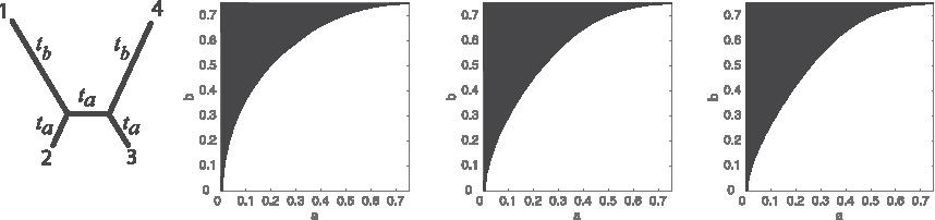
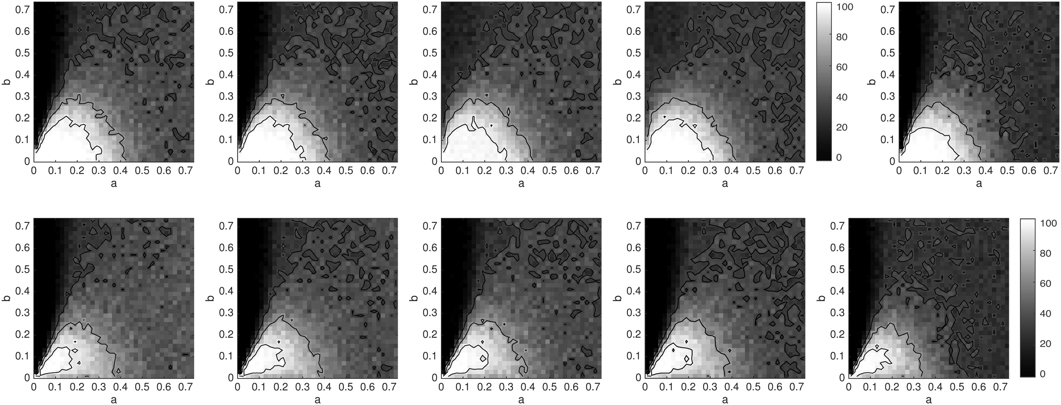
We follow the framework suggested by Felsenstein (1978). We consider an unrooted four-leaf tree with topology 12|34. Two branch lengths, t_a and t_b, each ranging over the interval (0, ∞), are used, with t_a on edges 2|134, 3|124, and 12|34 and t_b on the edges 1|234 and 4|123. This tree is depicted in Figure 1. The branch lengths are transformed to probabilities, a and b, in (0, 0.75), probabilities that bases at a site differ at opposite ends of a branch.

OPEN IN VIEWER

FIG. 1.

The white region is the zone of consistency for tree inference using the naive k-mer distance combined with the four-point condition. From left to right, k = 1, 3, and 5. The usual Felsenstein Zone is in the upper left.

Consider the naive k-mer method that uses d as a distance together with the four-point condition (or equivalently, NJ) to infer a tree topology. To analyze its behavior, we must first relate the expected values of \documentclass{aastex}\usepackage{amsbsy}\usepackage{amsfonts}\usepackage{amssymb}\usepackage{bm}\usepackage{mathrsfs}\usepackage{pifont}\usepackage{stmaryrd}\usepackage{textcomp}\usepackage{portland, xspace}\usepackage{amsmath, amsxtra}\pagestyle{empty}\DeclareMathSizes{10}{9}{7}{6}\begin{document} \begin{align*} d = 2 ( n - k + 1 ) \left( { 1 - { { \left( { \frac { { 1 + 3 \exp ( - 4t / 3 ) } } { 4 } } \right) } ^k } } \right) , \end{align*} \end{document}

for each taxon pair to the underlying branch parameters, a and b. As a is the probability that some change from the current state is made along the edge of scaled length t_a [y from Eq. (4)], we have that the diagonal element from the associated JC transition matrix is \documentclass{aastex}\usepackage{amsbsy}\usepackage{amsfonts}\usepackage{amssymb}\usepackage{bm}\usepackage{mathrsfs}\usepackage{pifont}\usepackage{stmaryrd}\usepackage{textcomp}\usepackage{portland, xspace}\usepackage{amsmath, amsxtra}\pagestyle{empty}\DeclareMathSizes{10}{9}{7}{6}\begin{document} \begin{align*} 1 - a = \frac { { 1 + 3 \exp ( - 4 { t_a } / 3 ) } } { 4 } \tag { 6 } \end{align*} \end{document}

and thus \documentclass{aastex}\usepackage{amsbsy}\usepackage{amsfonts}\usepackage{amssymb}\usepackage{bm}\usepackage{mathrsfs}\usepackage{pifont}\usepackage{stmaryrd}\usepackage{textcomp}\usepackage{portland, xspace}\usepackage{amsmath, amsxtra}\pagestyle{empty}\DeclareMathSizes{10}{9}{7}{6}\begin{document} \begin{align*} { t_a } = - \frac { 3 } { 4 } \ln \left( { 1 - \frac { 4 } { 3 } a } \right). \end{align*} \end{document}

Similar arithmetic gives the formula for t_b.

This yields the following formulas for the expected distance in terms of the parameters a and b: \documentclass{aastex}\usepackage{amsbsy}\usepackage{amsfonts}\usepackage{amssymb}\usepackage{bm}\usepackage{mathrsfs}\usepackage{pifont}\usepackage{stmaryrd}\usepackage{textcomp}\usepackage{portland, xspace}\usepackage{amsmath, amsxtra}\pagestyle{empty}\DeclareMathSizes{10}{9}{7}{6}\begin{document} \begin{align*} & { d_ { 12 } } \ =\ { d_ { 34 } } \ \ =\ \ 2 ( n - k + 1 ) \left( { 1 - { { \left( { \frac { { 1 + 3 ( 1 - \frac { 4 } { 3 } a ) ( 1 - \frac { 4 } { 3 } b ) } } { 4 } } \right) } ^k } } \right) , \\ & { d_ { 13 } } \ =\ { d_ { 24 } } \ \ =\ \ 2 ( n - k + 1 ) \left( { 1 - { { \left( { \frac { { 1 + 3 ( 1 - \frac { 4 } { 3 } a { ) ^2 } ( 1 - \frac { 4 } { 3 } b ) } } { 4 } } \right) } ^k } } \right) , \\ & \qquad \quad { \mkern 1mu } { d_ { 14 } } \ \ =\ \ 2 ( n - k + 1 ) \left( { 1 - { { \left( { \frac { { 1 + 3 ( 1 - \frac { 4 } { 3 } a ) ( 1 - \frac { 4 } { 3 } b { ) ^2 } } } { 4 } } \right) } ^k } } \right) , \\ & \qquad \quad { \mkern 1mu } { d_ { 23 } } \ \ =\ \ 2 ( n - k + 1 ) \left( { 1 - { { \left( { \frac { { 1 + 3 ( 1 - \frac { 4 } { 3 } a { ) ^3 } } } { 4 } } \right) } ^k } } \right). \\ \end{align*} \end{document}

To construct correctly the unique true tree 12|34 using the four-point condition or NJ, requires that these distances satisfy \documentclass{aastex}\usepackage{amsbsy}\usepackage{amsfonts}\usepackage{amssymb}\usepackage{bm}\usepackage{mathrsfs}\usepackage{pifont}\usepackage{stmaryrd}\usepackage{textcomp}\usepackage{portland, xspace}\usepackage{amsmath, amsxtra}\pagestyle{empty}\DeclareMathSizes{10}{9}{7}{6}\begin{document} \begin{align*} {d_{12}} + {d_{34}} < \min ( {d_{13}} + {d_{24}}, \ {d_{14}} + {d_{23}} ). \end{align*} \end{document}

Note that \documentclass{aastex}\usepackage{amsbsy}\usepackage{amsfonts}\usepackage{amssymb}\usepackage{bm}\usepackage{mathrsfs}\usepackage{pifont}\usepackage{stmaryrd}\usepackage{textcomp}\usepackage{portland, xspace}\usepackage{amsmath, amsxtra}\pagestyle{empty}\DeclareMathSizes{10}{9}{7}{6}\begin{document} $${d_{12}} + {d_{34}} < {d_{13}} + {d_{24}}$$ \end{document} for all \documentclass{aastex}\usepackage{amsbsy}\usepackage{amsfonts}\usepackage{amssymb}\usepackage{bm}\usepackage{mathrsfs}\usepackage{pifont}\usepackage{stmaryrd}\usepackage{textcomp}\usepackage{portland, xspace}\usepackage{amsmath, amsxtra}\pagestyle{empty}\DeclareMathSizes{10}{9}{7}{6}\begin{document} $$a > 0$$ \end{document} , so we focus on the condition \documentclass{aastex}\usepackage{amsbsy}\usepackage{amsfonts}\usepackage{amssymb}\usepackage{bm}\usepackage{mathrsfs}\usepackage{pifont}\usepackage{stmaryrd}\usepackage{textcomp}\usepackage{portland, xspace}\usepackage{amsmath, amsxtra}\pagestyle{empty}\DeclareMathSizes{10}{9}{7}{6}\begin{document} \begin{align*} {d_{12}} + {d_{34}} < {d_{14}} + {d_{23}}. \end{align*} \end{document}

Using the formulas above, this becomes \documentclass{aastex}\usepackage{amsbsy}\usepackage{amsfonts}\usepackage{amssymb}\usepackage{bm}\usepackage{mathrsfs}\usepackage{pifont}\usepackage{stmaryrd}\usepackage{textcomp}\usepackage{portland, xspace}\usepackage{amsmath, amsxtra}\pagestyle{empty}\DeclareMathSizes{10}{9}{7}{6}\begin{document} \begin{align*} 2 { \left( { 1 + 3 ( 1 - \frac { 4 } { 3 } a ) ( 1 - \frac { 4 } { 3 } b ) } \right) ^k } > { \left( { 1 + 3 ( 1 - \frac { 4 } { 3 } a ) ( 1 - \frac { 4 } { 3 } b { ) ^2 } } \right) ^k } + { \left( { 1 + 3 ( 1 - \frac { 4 } { 3 } a { ) ^3 } } \right) ^k } . \end{align*} \end{document}

The values of a and b for which this is satisfied are shown by the white regions in Figure 1 for k = 1, 3, and 5. As k increases, the white regions change; when k = 1, the boundary curve is a circle, and as k →∞, it approaches a parabola with vertex in the upper right corner, passing through the lower left. Note that the white region indicates where the naive k-mer distance inference behaves well, provided one knows d exactly—in practice one only has an estimate of d and should not expect even this good behavior.

In contrast, using the corrected JC k-mer distance from Equation (2) to make diagrams analogous to those of Figure 1 would show the entire square white. If d were known exactly, inference would be perfect. The corrected distances lead to statistically consistent distance methods on four-taxon trees. More generally, our argument in Section 2 shows that we can use Theorem 2.1 to derive statistically consistent estimates for the evolutionary time between species when we have a known time-reversible rate matrix Q.

4. Identifiability of Indel-Free Model Parameters

The results in Section 2 prove that with knowledge of the stationary base frequency π of an unknown Markov matrix, M, describing base substitutions from one sequence to another, tr M is identifiable from the joint distribution of k-mer counts in the two sequences. If one assumes a continuous-time model with M = exp(Qt) and Q a known time-reversible rate matrix, then this is sufficient to identify lengths t between taxa on the tree. As a consequence, with Q known, the metric phylogenetic tree relating many taxa is identifiable.

In fact, more is true: π and M are identifiable from 1-mer count distributions as well. This is the result in the next proposition, which in addition to being interesting in its own right, plays a role in the proof of Theorem 2.1. Its proof appears in Section 9. Note that in this result, we do not assume that base frequency distributions π_i are the stationary vectors of the Markov matrix.

Proposition 4.1. From the joint distribution of 1-mer count vectors, \documentclass{aastex}\usepackage{amsbsy}\usepackage{amsfonts}\usepackage{amssymb}\usepackage{bm}\usepackage{mathrsfs}\usepackage{pifont}\usepackage{stmaryrd}\usepackage{textcomp}\usepackage{portland, xspace}\usepackage{amsmath, amsxtra}\pagestyle{empty}\DeclareMathSizes{10}{9}{7}{6}\begin{document} $${X_1}$$ \end{document} and \documentclass{aastex}\usepackage{amsbsy}\usepackage{amsfonts}\usepackage{amssymb}\usepackage{bm}\usepackage{mathrsfs}\usepackage{pifont}\usepackage{stmaryrd}\usepackage{textcomp}\usepackage{portland, xspace}\usepackage{amsmath, amsxtra}\pagestyle{empty}\DeclareMathSizes{10}{9}{7}{6}\begin{document} $${X_2}$$ \end{document} , of two sequences, \documentclass{aastex}\usepackage{amsbsy}\usepackage{amsfonts}\usepackage{amssymb}\usepackage{bm}\usepackage{mathrsfs}\usepackage{pifont}\usepackage{stmaryrd}\usepackage{textcomp}\usepackage{portland, xspace}\usepackage{amsmath, amsxtra}\pagestyle{empty}\DeclareMathSizes{10}{9}{7}{6}\begin{document} $${S_1}$$ \end{document} and \documentclass{aastex}\usepackage{amsbsy}\usepackage{amsfonts}\usepackage{amssymb}\usepackage{bm}\usepackage{mathrsfs}\usepackage{pifont}\usepackage{stmaryrd}\usepackage{textcomp}\usepackage{portland, xspace}\usepackage{amsmath, amsxtra}\pagestyle{empty}\DeclareMathSizes{10}{9}{7}{6}\begin{document} $${S_2}$$ \end{document} , of length \documentclass{aastex}\usepackage{amsbsy}\usepackage{amsfonts}\usepackage{amssymb}\usepackage{bm}\usepackage{mathrsfs}\usepackage{pifont}\usepackage{stmaryrd}\usepackage{textcomp}\usepackage{portland, xspace}\usepackage{amsmath, amsxtra}\pagestyle{empty}\DeclareMathSizes{10}{9}{7}{6}\begin{document} $$n$$ \end{document} , one can identify the distributions, \documentclass{aastex}\usepackage{amsbsy}\usepackage{amsfonts}\usepackage{amssymb}\usepackage{bm}\usepackage{mathrsfs}\usepackage{pifont}\usepackage{stmaryrd}\usepackage{textcomp}\usepackage{portland, xspace}\usepackage{amsmath, amsxtra}\pagestyle{empty}\DeclareMathSizes{10}{9}{7}{6}\begin{document} $${ \pi _1}$$ \end{document} and \documentclass{aastex}\usepackage{amsbsy}\usepackage{amsfonts}\usepackage{amssymb}\usepackage{bm}\usepackage{mathrsfs}\usepackage{pifont}\usepackage{stmaryrd}\usepackage{textcomp}\usepackage{portland, xspace}\usepackage{amsmath, amsxtra}\pagestyle{empty}\DeclareMathSizes{10}{9}{7}{6}\begin{document} $${ \pi _2}$$ \end{document} , of bases in each sequence and the joint distribution \documentclass{aastex}\usepackage{amsbsy}\usepackage{amsfonts}\usepackage{amssymb}\usepackage{bm}\usepackage{mathrsfs}\usepackage{pifont}\usepackage{stmaryrd}\usepackage{textcomp}\usepackage{portland, xspace}\usepackage{amsmath, amsxtra}\pagestyle{empty}\DeclareMathSizes{10}{9}{7}{6}\begin{document} $$P = { \rm{diag}} ( { \pi _1} ) M$$ \end{document} of bases at a single site in the two sequences. Specifically, \documentclass{aastex}\usepackage{amsbsy}\usepackage{amsfonts}\usepackage{amssymb}\usepackage{bm}\usepackage{mathrsfs}\usepackage{pifont}\usepackage{stmaryrd}\usepackage{textcomp}\usepackage{portland, xspace}\usepackage{amsmath, amsxtra}\pagestyle{empty}\DeclareMathSizes{10}{9}{7}{6}\begin{document} $$ { \pi _i } = \frac { 1 } { n } { \mathbb E } [ { X_i } ]$$ \end{document} , and for \documentclass{aastex}\usepackage{amsbsy}\usepackage{amsfonts}\usepackage{amssymb}\usepackage{bm}\usepackage{mathrsfs}\usepackage{pifont}\usepackage{stmaryrd}\usepackage{textcomp}\usepackage{portland, xspace}\usepackage{amsmath, amsxtra}\pagestyle{empty}\DeclareMathSizes{10}{9}{7}{6}\begin{document} $$w, \ u \in [ L ]$$ \end{document} , \documentclass{aastex}\usepackage{amsbsy}\usepackage{amsfonts}\usepackage{amssymb}\usepackage{bm}\usepackage{mathrsfs}\usepackage{pifont}\usepackage{stmaryrd}\usepackage{textcomp}\usepackage{portland, xspace}\usepackage{amsmath, amsxtra}\pagestyle{empty}\DeclareMathSizes{10}{9}{7}{6}\begin{document} \begin{align*} { P_ { wu } } = \frac { 1 } { 2 } \left( { \pi _1^w + \pi _2^u - \frac { { \pi _1^w \pi _2^u } } { n } { \mathbb E } \left[ { { { \left( { { \frac { X_1^w } { \pi _1^w } } - { \frac { X_2^u } { \pi _2^u } } } \right) } ^2 } } \right] } \right). \end{align*} \end{document}

The formula for \documentclass{aastex}\usepackage{amsbsy}\usepackage{amsfonts}\usepackage{amssymb}\usepackage{bm}\usepackage{mathrsfs}\usepackage{pifont}\usepackage{stmaryrd}\usepackage{textcomp}\usepackage{portland, xspace}\usepackage{amsmath, amsxtra}\pagestyle{empty}\DeclareMathSizes{10}{9}{7}{6}\begin{document} $${P_{wu}}$$ \end{document} in this proposition ultimately underlies our suggested practical inference method. However, there is a simpler formula, applying for any \documentclass{aastex}\usepackage{amsbsy}\usepackage{amsfonts}\usepackage{amssymb}\usepackage{bm}\usepackage{mathrsfs}\usepackage{pifont}\usepackage{stmaryrd}\usepackage{textcomp}\usepackage{portland, xspace}\usepackage{amsmath, amsxtra}\pagestyle{empty}\DeclareMathSizes{10}{9}{7}{6}\begin{document} $$k$$ \end{document} , showing that from a joint \documentclass{aastex}\usepackage{amsbsy}\usepackage{amsfonts}\usepackage{amssymb}\usepackage{bm}\usepackage{mathrsfs}\usepackage{pifont}\usepackage{stmaryrd}\usepackage{textcomp}\usepackage{portland, xspace}\usepackage{amsmath, amsxtra}\pagestyle{empty}\DeclareMathSizes{10}{9}{7}{6}\begin{document} $$k$$ \end{document} -mer count vector distribution, one can identify the joint probabilities \documentclass{aastex}\usepackage{amsbsy}\usepackage{amsfonts}\usepackage{amssymb}\usepackage{bm}\usepackage{mathrsfs}\usepackage{pifont}\usepackage{stmaryrd}\usepackage{textcomp}\usepackage{portland, xspace}\usepackage{amsmath, amsxtra}\pagestyle{empty}\DeclareMathSizes{10}{9}{7}{6}\begin{document} $${P_{wu}}$$ \end{document} : For sequences of length \documentclass{aastex}\usepackage{amsbsy}\usepackage{amsfonts}\usepackage{amssymb}\usepackage{bm}\usepackage{mathrsfs}\usepackage{pifont}\usepackage{stmaryrd}\usepackage{textcomp}\usepackage{portland, xspace}\usepackage{amsmath, amsxtra}\pagestyle{empty}\DeclareMathSizes{10}{9}{7}{6}\begin{document} $$n$$ \end{document} and the particular \documentclass{aastex}\usepackage{amsbsy}\usepackage{amsfonts}\usepackage{amssymb}\usepackage{bm}\usepackage{mathrsfs}\usepackage{pifont}\usepackage{stmaryrd}\usepackage{textcomp}\usepackage{portland, xspace}\usepackage{amsmath, amsxtra}\pagestyle{empty}\DeclareMathSizes{10}{9}{7}{6}\begin{document} $$k$$ \end{document} -mers, \documentclass{aastex}\usepackage{amsbsy}\usepackage{amsfonts}\usepackage{amssymb}\usepackage{bm}\usepackage{mathrsfs}\usepackage{pifont}\usepackage{stmaryrd}\usepackage{textcomp}\usepackage{portland, xspace}\usepackage{amsmath, amsxtra}\pagestyle{empty}\DeclareMathSizes{10}{9}{7}{6}\begin{document} $$W = www \ldots w$$ \end{document} and \documentclass{aastex}\usepackage{amsbsy}\usepackage{amsfonts}\usepackage{amssymb}\usepackage{bm}\usepackage{mathrsfs}\usepackage{pifont}\usepackage{stmaryrd}\usepackage{textcomp}\usepackage{portland, xspace}\usepackage{amsmath, amsxtra}\pagestyle{empty}\DeclareMathSizes{10}{9}{7}{6}\begin{document} $$U = uuu \ldots u$$ \end{document} , \documentclass{aastex}\usepackage{amsbsy}\usepackage{amsfonts}\usepackage{amssymb}\usepackage{bm}\usepackage{mathrsfs}\usepackage{pifont}\usepackage{stmaryrd}\usepackage{textcomp}\usepackage{portland, xspace}\usepackage{amsmath, amsxtra}\pagestyle{empty}\DeclareMathSizes{10}{9}{7}{6}\begin{document} \begin{align*} { \rm{Prob}} ( X_1^W = n - k + 1 , \ X_2^U = n - k + 1 ) = ( {P_{wu}}{ ) ^n}. \end{align*} \end{document}

Of course, the method of estimation suggested by this approach is useless in practice since it is based on events that are rarely, if ever, observed.

Nonetheless, since \documentclass{aastex}\usepackage{amsbsy}\usepackage{amsfonts}\usepackage{amssymb}\usepackage{bm}\usepackage{mathrsfs}\usepackage{pifont}\usepackage{stmaryrd}\usepackage{textcomp}\usepackage{portland, xspace}\usepackage{amsmath, amsxtra}\pagestyle{empty}\DeclareMathSizes{10}{9}{7}{6}\begin{document} $$P$$ \end{document} and \documentclass{aastex}\usepackage{amsbsy}\usepackage{amsfonts}\usepackage{amssymb}\usepackage{bm}\usepackage{mathrsfs}\usepackage{pifont}\usepackage{stmaryrd}\usepackage{textcomp}\usepackage{portland, xspace}\usepackage{amsmath, amsxtra}\pagestyle{empty}\DeclareMathSizes{10}{9}{7}{6}\begin{document} $${ \pi _1}$$ \end{document} can be found from the joint distribution of \documentclass{aastex}\usepackage{amsbsy}\usepackage{amsfonts}\usepackage{amssymb}\usepackage{bm}\usepackage{mathrsfs}\usepackage{pifont}\usepackage{stmaryrd}\usepackage{textcomp}\usepackage{portland, xspace}\usepackage{amsmath, amsxtra}\pagestyle{empty}\DeclareMathSizes{10}{9}{7}{6}\begin{document} $${X_1}$$ \end{document} and \documentclass{aastex}\usepackage{amsbsy}\usepackage{amsfonts}\usepackage{amssymb}\usepackage{bm}\usepackage{mathrsfs}\usepackage{pifont}\usepackage{stmaryrd}\usepackage{textcomp}\usepackage{portland, xspace}\usepackage{amsmath, amsxtra}\pagestyle{empty}\DeclareMathSizes{10}{9}{7}{6}\begin{document} $${X_2}$$ \end{document} for any \documentclass{aastex}\usepackage{amsbsy}\usepackage{amsfonts}\usepackage{amssymb}\usepackage{bm}\usepackage{mathrsfs}\usepackage{pifont}\usepackage{stmaryrd}\usepackage{textcomp}\usepackage{portland, xspace}\usepackage{amsmath, amsxtra}\pagestyle{empty}\DeclareMathSizes{10}{9}{7}{6}\begin{document} $$k$$ \end{document} , the transition matrix \documentclass{aastex}\usepackage{amsbsy}\usepackage{amsfonts}\usepackage{amssymb}\usepackage{bm}\usepackage{mathrsfs}\usepackage{pifont}\usepackage{stmaryrd}\usepackage{textcomp}\usepackage{portland, xspace}\usepackage{amsmath, amsxtra}\pagestyle{empty}\DeclareMathSizes{10}{9}{7}{6}\begin{document} $$M = { \rm{diag}}{ ( { \pi _1} ) ^{ - 1}}P$$ \end{document} is also identifiable. In the continuous-time model setting, where \documentclass{aastex}\usepackage{amsbsy}\usepackage{amsfonts}\usepackage{amssymb}\usepackage{bm}\usepackage{mathrsfs}\usepackage{pifont}\usepackage{stmaryrd}\usepackage{textcomp}\usepackage{portland, xspace}\usepackage{amsmath, amsxtra}\pagestyle{empty}\DeclareMathSizes{10}{9}{7}{6}\begin{document} $$M = \exp ( Qt )$$ \end{document} , \documentclass{aastex}\usepackage{amsbsy}\usepackage{amsfonts}\usepackage{amssymb}\usepackage{bm}\usepackage{mathrsfs}\usepackage{pifont}\usepackage{stmaryrd}\usepackage{textcomp}\usepackage{portland, xspace}\usepackage{amsmath, amsxtra}\pagestyle{empty}\DeclareMathSizes{10}{9}{7}{6}\begin{document} $$Q$$ \end{document} can be found, first up to a scalar multiple, and then normalized. Putting this together yields the following.

Theorem 4.2. For an indel-free GTR model, all parameters, both numerical ones and tree topology, can be identified from pairwise joint k-mer count distributions.

If we consider sequences three at a time, rather than pairwise, we obtain an analog of Proposition 4.1, again without assuming stationarity. This new result is based on third moments, rather than second, and its proof is given in Section 9.

Proposition 4.3. For a three-leaf tree, the joint distribution \documentclass{aastex}\usepackage{amsbsy}\usepackage{amsfonts}\usepackage{amssymb}\usepackage{bm}\usepackage{mathrsfs}\usepackage{pifont}\usepackage{stmaryrd}\usepackage{textcomp}\usepackage{portland, xspace}\usepackage{amsmath, amsxtra}\pagestyle{empty}\DeclareMathSizes{10}{9}{7}{6}\begin{document} $$P = ( {P_{uvw}} )$$ \end{document} of site patterns is identifiable from the joint 1-mer count vector distributions of the three taxa. Specifically, define a random variable \documentclass{aastex}\usepackage{amsbsy}\usepackage{amsfonts}\usepackage{amssymb}\usepackage{bm}\usepackage{mathrsfs}\usepackage{pifont}\usepackage{stmaryrd}\usepackage{textcomp}\usepackage{portland, xspace}\usepackage{amsmath, amsxtra}\pagestyle{empty}\DeclareMathSizes{10}{9}{7}{6}\begin{document} \begin{align*} {Y_{uvw}} = \alpha X_1^u + \beta X_2^v + \gamma X_3^w , \end{align*} \end{document}

where α, β, and γ are constants chosen so \documentclass{aastex}\usepackage{amsbsy}\usepackage{amsfonts}\usepackage{amssymb}\usepackage{bm}\usepackage{mathrsfs}\usepackage{pifont}\usepackage{stmaryrd}\usepackage{textcomp}\usepackage{portland, xspace}\usepackage{amsmath, amsxtra}\pagestyle{empty}\DeclareMathSizes{10}{9}{7}{6}\begin{document} \begin{align*} \alpha \pi _1^u + \beta \pi _2^v + \gamma \pi _3^w = 0. \end{align*} \end{document}

Then,

where the pairwise marginal distributions, P_uv+, P_u+w, and P_+vw, in Equation (7) are identifiable by Proposition 4.1.

Proposition 4.3 is significant in that it establishes that the distribution of 1-mer counts contains enough information to identify parameters of more general models than our preceding arguments allow. Recall, for instance, parameters for the General Markov (GM) model, in which the base substitution process on each edge of the tree can be specified by a different Markov matrix, are identifiable from the marginalization of the site pattern distribution to three-taxon sets (Chang, 1996), but are not identifiable from pairwise marginalizations. In the present context of k-mers, we obtain the following.

Corollary 4.4. For an indel-free GM model, all parameters, both numerical ones and tree topology, are identifiable from the joint 1-mer count vector distributions on n taxa.

5. Practical k-mer Distances Between Sequences

In this section, we apply the results of Section 2 to develop practical methods for estimating pairwise distances between sequences. Those derivations were made under the assumption that sequences evolved in the absence of an indel process and thus that sequences could be unambiguously aligned. In practice, however, we desire a method of distance estimation that can be applied in the presence of a mild indel process, without a precise alignment. Although this violates our model assumptions, in Section 6, we use simulations to investigate how robust our resulting method is to such a violation.

Assuming a JC process of site substitution and no indel process, Formula (2) of Corollary 2.2 suggests a natural definition for a distance, provided we have a good method of approximating \documentclass{aastex}\usepackage{amsbsy}\usepackage{amsfonts}\usepackage{amssymb}\usepackage{bm}\usepackage{mathrsfs}\usepackage{pifont}\usepackage{stmaryrd}\usepackage{textcomp}\usepackage{portland, xspace}\usepackage{amsmath, amsxtra}\pagestyle{empty}\DeclareMathSizes{10}{9}{7}{6}\begin{document} $$d = {\mathbb E} \left[ { \parallel {X_1} - {X_2} \parallel _2^2} \right]$$ \end{document} . If the observed values of the random variables, X₁ and X₂, are denoted in lower case, so x₁ and x₂ are observed k-mer count vectors, then one could simply compute \documentclass{aastex}\usepackage{amsbsy}\usepackage{amsfonts}\usepackage{amssymb}\usepackage{bm}\usepackage{mathrsfs}\usepackage{pifont}\usepackage{stmaryrd}\usepackage{textcomp}\usepackage{portland, xspace}\usepackage{amsmath, amsxtra}\pagestyle{empty}\DeclareMathSizes{10}{9}{7}{6}\begin{document} \begin{align*} \parallel {x_1} - {x_2} \parallel _2^2 \ = \mathop \sum \limits_{W \in {{ [ L ] }^k}} { \left( {x_1^W - x_2^W} \right) ^2} \tag{8} \end{align*} \end{document}

as a point estimate for d. This is a very poor estimate for the expected value, however, since only one sample ( \documentclass{aastex}\usepackage{amsbsy}\usepackage{amsfonts}\usepackage{amssymb}\usepackage{bm}\usepackage{mathrsfs}\usepackage{pifont}\usepackage{stmaryrd}\usepackage{textcomp}\usepackage{portland, xspace}\usepackage{amsmath, amsxtra}\pagestyle{empty}\DeclareMathSizes{10}{9}{7}{6}\begin{document} $$\parallel {x_1} - {x_2}{ \parallel ^2}$$ \end{document} ) is used to estimate a mean. Indeed, this estimate has large variance. Moreover, naively increasing sequence length (number of k-mers) would do nothing to address the fundamental problem of needing more samples to estimate a mean well.

To obtain a better estimate of d, with smaller variance, we instead subdivide the two sequences into a fixed number B of contiguous blocks. Assuming for 1 ≤ i ≤ B that the ith blocks of the two sequences are at least roughly orthologous, we compute the k-mer frequencies x_j,i for each block i in sequence j. Then, the values of \documentclass{aastex}\usepackage{amsbsy}\usepackage{amsfonts}\usepackage{amssymb}\usepackage{bm}\usepackage{mathrsfs}\usepackage{pifont}\usepackage{stmaryrd}\usepackage{textcomp}\usepackage{portland, xspace}\usepackage{amsmath, amsxtra}\pagestyle{empty}\DeclareMathSizes{10}{9}{7}{6}\begin{document} $$\parallel {x_{1 , i}} - {x_{2 , i}} \parallel _2^2$$ \end{document} for the B blocks can be averaged to estimate d. In this framework, we are adopting the approach introduced by Daskalakis and Roch (2013).

We have in mind two scenarios for using this approach on data, which are displayed in Figure 2. The first is under the assumption that if indels occurred, they were distributed evenly over the sequences. Then, if the blocks are defined as a fixed fraction of the full sequence lengths, most of the sites in the ith blocks of the two sequences will be orthologous. The second is that the blocks arise naturally in the data; for instance, if a dataset consists of multiple genes, then each gene can be treated as a block. In this case, the point estimates for each gene would be averaged over all genes, making appropriate adjustments for their varying lengths.

OPEN IN VIEWER

FIG. 2.

On the left, two sequences, in which blocks i are roughly orthologous, perhaps due to a uniform indel process. On the right, two genomes, in which genes serve as blocks for data analysis.

To be precise, in addition to specifying \documentclass{aastex}\usepackage{amsbsy}\usepackage{amsfonts}\usepackage{amssymb}\usepackage{bm}\usepackage{mathrsfs}\usepackage{pifont}\usepackage{stmaryrd}\usepackage{textcomp}\usepackage{portland, xspace}\usepackage{amsmath, amsxtra}\pagestyle{empty}\DeclareMathSizes{10}{9}{7}{6}\begin{document} $$k$$ \end{document} , under the first scenario, we must also specify a number \documentclass{aastex}\usepackage{amsbsy}\usepackage{amsfonts}\usepackage{amssymb}\usepackage{bm}\usepackage{mathrsfs}\usepackage{pifont}\usepackage{stmaryrd}\usepackage{textcomp}\usepackage{portland, xspace}\usepackage{amsmath, amsxtra}\pagestyle{empty}\DeclareMathSizes{10}{9}{7}{6}\begin{document} $$B$$ \end{document} of blocks to be used in our calculations. To subdivide a sequence \documentclass{aastex}\usepackage{amsbsy}\usepackage{amsfonts}\usepackage{amssymb}\usepackage{bm}\usepackage{mathrsfs}\usepackage{pifont}\usepackage{stmaryrd}\usepackage{textcomp}\usepackage{portland, xspace}\usepackage{amsmath, amsxtra}\pagestyle{empty}\DeclareMathSizes{10}{9}{7}{6}\begin{document} $${S_j}$$ \end{document} of length \documentclass{aastex}\usepackage{amsbsy}\usepackage{amsfonts}\usepackage{amssymb}\usepackage{bm}\usepackage{mathrsfs}\usepackage{pifont}\usepackage{stmaryrd}\usepackage{textcomp}\usepackage{portland, xspace}\usepackage{amsmath, amsxtra}\pagestyle{empty}\DeclareMathSizes{10}{9}{7}{6}\begin{document} $${n_j}$$ \end{document} as uniformly as possible, each block will have length \documentclass{aastex}\usepackage{amsbsy}\usepackage{amsfonts}\usepackage{amssymb}\usepackage{bm}\usepackage{mathrsfs}\usepackage{pifont}\usepackage{stmaryrd}\usepackage{textcomp}\usepackage{portland, xspace}\usepackage{amsmath, amsxtra}\pagestyle{empty}\DeclareMathSizes{10}{9}{7}{6}\begin{document} $${n_{j , i}} = {n_j} / B$$ \end{document} , suitably rounded for \documentclass{aastex}\usepackage{amsbsy}\usepackage{amsfonts}\usepackage{amssymb}\usepackage{bm}\usepackage{mathrsfs}\usepackage{pifont}\usepackage{stmaryrd}\usepackage{textcomp}\usepackage{portland, xspace}\usepackage{amsmath, amsxtra}\pagestyle{empty}\DeclareMathSizes{10}{9}{7}{6}\begin{document} $$1 \le i \le B$$ \end{document} , so block lengths for a single sequence can differ at most by one. Under the second scenario, using natural blocks such as genes, the length \documentclass{aastex}\usepackage{amsbsy}\usepackage{amsfonts}\usepackage{amssymb}\usepackage{bm}\usepackage{mathrsfs}\usepackage{pifont}\usepackage{stmaryrd}\usepackage{textcomp}\usepackage{portland, xspace}\usepackage{amsmath, amsxtra}\pagestyle{empty}\DeclareMathSizes{10}{9}{7}{6}\begin{document} $${n_{j , i}}$$ \end{document} is specified by the data and will vary more widely.

Now, for block \documentclass{aastex}\usepackage{amsbsy}\usepackage{amsfonts}\usepackage{amssymb}\usepackage{bm}\usepackage{mathrsfs}\usepackage{pifont}\usepackage{stmaryrd}\usepackage{textcomp}\usepackage{portland, xspace}\usepackage{amsmath, amsxtra}\pagestyle{empty}\DeclareMathSizes{10}{9}{7}{6}\begin{document} $$i$$ \end{document} in sequence \documentclass{aastex}\usepackage{amsbsy}\usepackage{amsfonts}\usepackage{amssymb}\usepackage{bm}\usepackage{mathrsfs}\usepackage{pifont}\usepackage{stmaryrd}\usepackage{textcomp}\usepackage{portland, xspace}\usepackage{amsmath, amsxtra}\pagestyle{empty}\DeclareMathSizes{10}{9}{7}{6}\begin{document} $$j$$ \end{document} , let \documentclass{aastex}\usepackage{amsbsy}\usepackage{amsfonts}\usepackage{amssymb}\usepackage{bm}\usepackage{mathrsfs}\usepackage{pifont}\usepackage{stmaryrd}\usepackage{textcomp}\usepackage{portland, xspace}\usepackage{amsmath, amsxtra}\pagestyle{empty}\DeclareMathSizes{10}{9}{7}{6}\begin{document} $${x_{j , i}}$$ \end{document} be the \documentclass{aastex}\usepackage{amsbsy}\usepackage{amsfonts}\usepackage{amssymb}\usepackage{bm}\usepackage{mathrsfs}\usepackage{pifont}\usepackage{stmaryrd}\usepackage{textcomp}\usepackage{portland, xspace}\usepackage{amsmath, amsxtra}\pagestyle{empty}\DeclareMathSizes{10}{9}{7}{6}\begin{document} $$k$$ \end{document} -mer count vector and \documentclass{aastex}\usepackage{amsbsy}\usepackage{amsfonts}\usepackage{amssymb}\usepackage{bm}\usepackage{mathrsfs}\usepackage{pifont}\usepackage{stmaryrd}\usepackage{textcomp}\usepackage{portland, xspace}\usepackage{amsmath, amsxtra}\pagestyle{empty}\DeclareMathSizes{10}{9}{7}{6}\begin{document} $${ \mu _{j , i}} = ( {n_{j , i}} - k + {1 ) / 4^k}$$ \end{document} the mean \documentclass{aastex}\usepackage{amsbsy}\usepackage{amsfonts}\usepackage{amssymb}\usepackage{bm}\usepackage{mathrsfs}\usepackage{pifont}\usepackage{stmaryrd}\usepackage{textcomp}\usepackage{portland, xspace}\usepackage{amsmath, amsxtra}\pagestyle{empty}\DeclareMathSizes{10}{9}{7}{6}\begin{document} $$k$$ \end{document} -mer count under the JC model. We define

Note that in this formula, both the centering of \documentclass{aastex}\usepackage{amsbsy}\usepackage{amsfonts}\usepackage{amssymb}\usepackage{bm}\usepackage{mathrsfs}\usepackage{pifont}\usepackage{stmaryrd}\usepackage{textcomp}\usepackage{portland, xspace}\usepackage{amsmath, amsxtra}\pagestyle{empty}\DeclareMathSizes{10}{9}{7}{6}\begin{document} $${x_{j , i}}$$ \end{document} by subtracting \documentclass{aastex}\usepackage{amsbsy}\usepackage{amsfonts}\usepackage{amssymb}\usepackage{bm}\usepackage{mathrsfs}\usepackage{pifont}\usepackage{stmaryrd}\usepackage{textcomp}\usepackage{portland, xspace}\usepackage{amsmath, amsxtra}\pagestyle{empty}\DeclareMathSizes{10}{9}{7}{6}\begin{document} $${ \mu _{j , i}}$$ \end{document} and the normalization by dividing by the square root of the number of \documentclass{aastex}\usepackage{amsbsy}\usepackage{amsfonts}\usepackage{amssymb}\usepackage{bm}\usepackage{mathrsfs}\usepackage{pifont}\usepackage{stmaryrd}\usepackage{textcomp}\usepackage{portland, xspace}\usepackage{amsmath, amsxtra}\pagestyle{empty}\DeclareMathSizes{10}{9}{7}{6}\begin{document} $$k$$ \end{document} -mers depend upon the length \documentclass{aastex}\usepackage{amsbsy}\usepackage{amsfonts}\usepackage{amssymb}\usepackage{bm}\usepackage{mathrsfs}\usepackage{pifont}\usepackage{stmaryrd}\usepackage{textcomp}\usepackage{portland, xspace}\usepackage{amsmath, amsxtra}\pagestyle{empty}\DeclareMathSizes{10}{9}{7}{6}\begin{document} $${n_{j , i}}$$ \end{document} . In the special situation where \documentclass{aastex}\usepackage{amsbsy}\usepackage{amsfonts}\usepackage{amssymb}\usepackage{bm}\usepackage{mathrsfs}\usepackage{pifont}\usepackage{stmaryrd}\usepackage{textcomp}\usepackage{portland, xspace}\usepackage{amsmath, amsxtra}\pagestyle{empty}\DeclareMathSizes{10}{9}{7}{6}\begin{document} $${n_{j , i}} = n$$ \end{document} for all \documentclass{aastex}\usepackage{amsbsy}\usepackage{amsfonts}\usepackage{amssymb}\usepackage{bm}\usepackage{mathrsfs}\usepackage{pifont}\usepackage{stmaryrd}\usepackage{textcomp}\usepackage{portland, xspace}\usepackage{amsmath, amsxtra}\pagestyle{empty}\DeclareMathSizes{10}{9}{7}{6}\begin{document} $$i , j$$ \end{document} , and hence \documentclass{aastex}\usepackage{amsbsy}\usepackage{amsfonts}\usepackage{amssymb}\usepackage{bm}\usepackage{mathrsfs}\usepackage{pifont}\usepackage{stmaryrd}\usepackage{textcomp}\usepackage{portland, xspace}\usepackage{amsmath, amsxtra}\pagestyle{empty}\DeclareMathSizes{10}{9}{7}{6}\begin{document} $${ \mu _{j , i}} = \mu$$ \end{document} , this reduces to \documentclass{aastex}\usepackage{amsbsy}\usepackage{amsfonts}\usepackage{amssymb}\usepackage{bm}\usepackage{mathrsfs}\usepackage{pifont}\usepackage{stmaryrd}\usepackage{textcomp}\usepackage{portland, xspace}\usepackage{amsmath, amsxtra}\pagestyle{empty}\DeclareMathSizes{10}{9}{7}{6}\begin{document} \begin{align*} \tilde d = \left( { \frac { 1 } { { n - k + 1 } } } \right) \frac { 1 } { B } \mathop \sum \limits_ { i = 1 } ^B \parallel { x_ { 1 , i } } - { x_ { 2 , i } } \parallel _2^2 \approx \frac { d } { { n - k + 1 } } . \end{align*} \end{document}

Comparing this estimate for \documentclass{aastex}\usepackage{amsbsy}\usepackage{amsfonts}\usepackage{amssymb}\usepackage{bm}\usepackage{mathrsfs}\usepackage{pifont}\usepackage{stmaryrd}\usepackage{textcomp}\usepackage{portland, xspace}\usepackage{amsmath, amsxtra}\pagestyle{empty}\DeclareMathSizes{10}{9}{7}{6}\begin{document} $$\tilde d$$ \end{document} with Equation (2), it is natural to define a JC \documentclass{aastex}\usepackage{amsbsy}\usepackage{amsfonts}\usepackage{amssymb}\usepackage{bm}\usepackage{mathrsfs}\usepackage{pifont}\usepackage{stmaryrd}\usepackage{textcomp}\usepackage{portland, xspace}\usepackage{amsmath, amsxtra}\pagestyle{empty}\DeclareMathSizes{10}{9}{7}{6}\begin{document} $$k$$ \end{document} -mer distance \documentclass{aastex}\usepackage{amsbsy}\usepackage{amsfonts}\usepackage{amssymb}\usepackage{bm}\usepackage{mathrsfs}\usepackage{pifont}\usepackage{stmaryrd}\usepackage{textcomp}\usepackage{portland, xspace}\usepackage{amsmath, amsxtra}\pagestyle{empty}\DeclareMathSizes{10}{9}{7}{6}\begin{document} $$d_{JC}^{k , B}$$ \end{document} , dependent on \documentclass{aastex}\usepackage{amsbsy}\usepackage{amsfonts}\usepackage{amssymb}\usepackage{bm}\usepackage{mathrsfs}\usepackage{pifont}\usepackage{stmaryrd}\usepackage{textcomp}\usepackage{portland, xspace}\usepackage{amsmath, amsxtra}\pagestyle{empty}\DeclareMathSizes{10}{9}{7}{6}\begin{document} $$k$$ \end{document} and \documentclass{aastex}\usepackage{amsbsy}\usepackage{amsfonts}\usepackage{amssymb}\usepackage{bm}\usepackage{mathrsfs}\usepackage{pifont}\usepackage{stmaryrd}\usepackage{textcomp}\usepackage{portland, xspace}\usepackage{amsmath, amsxtra}\pagestyle{empty}\DeclareMathSizes{10}{9}{7}{6}\begin{document} $$B$$ \end{document} , by \documentclass{aastex}\usepackage{amsbsy}\usepackage{amsfonts}\usepackage{amssymb}\usepackage{bm}\usepackage{mathrsfs}\usepackage{pifont}\usepackage{stmaryrd}\usepackage{textcomp}\usepackage{portland, xspace}\usepackage{amsmath, amsxtra}\pagestyle{empty}\DeclareMathSizes{10}{9}{7}{6}\begin{document} \begin{align*} d_ { JC } ^ { k , B } = - \frac { 3 } { 4 } \ln \left( { \frac { 4 } { 3 } \root k \of { 1 - \frac { { \tilde d } } { 2 } } - \frac { 1 } { 3 } } \right). \tag { 10 } \end{align*} \end{document}

We use this formula extensively in the simulations whose results are presented in the next section.

On examining Equation (10), it is unclear, a priori, which values of \documentclass{aastex}\usepackage{amsbsy}\usepackage{amsfonts}\usepackage{amssymb}\usepackage{bm}\usepackage{mathrsfs}\usepackage{pifont}\usepackage{stmaryrd}\usepackage{textcomp}\usepackage{portland, xspace}\usepackage{amsmath, amsxtra}\pagestyle{empty}\DeclareMathSizes{10}{9}{7}{6}\begin{document} $$k$$ \end{document} and \documentclass{aastex}\usepackage{amsbsy}\usepackage{amsfonts}\usepackage{amssymb}\usepackage{bm}\usepackage{mathrsfs}\usepackage{pifont}\usepackage{stmaryrd}\usepackage{textcomp}\usepackage{portland, xspace}\usepackage{amsmath, amsxtra}\pagestyle{empty}\DeclareMathSizes{10}{9}{7}{6}\begin{document} $$B$$ \end{document} will yield the best estimate for \documentclass{aastex}\usepackage{amsbsy}\usepackage{amsfonts}\usepackage{amssymb}\usepackage{bm}\usepackage{mathrsfs}\usepackage{pifont}\usepackage{stmaryrd}\usepackage{textcomp}\usepackage{portland, xspace}\usepackage{amsmath, amsxtra}\pagestyle{empty}\DeclareMathSizes{10}{9}{7}{6}\begin{document} $$d_{JC}^{k , B}$$ \end{document} . In the particular case that sequences evolved without an indel process, the lowest variance estimate of \documentclass{aastex}\usepackage{amsbsy}\usepackage{amsfonts}\usepackage{amssymb}\usepackage{bm}\usepackage{mathrsfs}\usepackage{pifont}\usepackage{stmaryrd}\usepackage{textcomp}\usepackage{portland, xspace}\usepackage{amsmath, amsxtra}\pagestyle{empty}\DeclareMathSizes{10}{9}{7}{6}\begin{document} $$d_{JC}^{k , B}$$ \end{document} is obtained by taking the largest number \documentclass{aastex}\usepackage{amsbsy}\usepackage{amsfonts}\usepackage{amssymb}\usepackage{bm}\usepackage{mathrsfs}\usepackage{pifont}\usepackage{stmaryrd}\usepackage{textcomp}\usepackage{portland, xspace}\usepackage{amsmath, amsxtra}\pagestyle{empty}\DeclareMathSizes{10}{9}{7}{6}\begin{document} $$B$$ \end{document} of samples, that is, each block has length \documentclass{aastex}\usepackage{amsbsy}\usepackage{amsfonts}\usepackage{amssymb}\usepackage{bm}\usepackage{mathrsfs}\usepackage{pifont}\usepackage{stmaryrd}\usepackage{textcomp}\usepackage{portland, xspace}\usepackage{amsmath, amsxtra}\pagestyle{empty}\DeclareMathSizes{10}{9}{7}{6}\begin{document} $$k$$ \end{document} (the smallest possible length, which allows \documentclass{aastex}\usepackage{amsbsy}\usepackage{amsfonts}\usepackage{amssymb}\usepackage{bm}\usepackage{mathrsfs}\usepackage{pifont}\usepackage{stmaryrd}\usepackage{textcomp}\usepackage{portland, xspace}\usepackage{amsmath, amsxtra}\pagestyle{empty}\DeclareMathSizes{10}{9}{7}{6}\begin{document} $$k$$ \end{document} -mers to be counted). However, in the presence of an evolutionary indel process, a true alignment of sequences would contain gaps, and such short block sizes would give poor results. For good performance, we need the \documentclass{aastex}\usepackage{amsbsy}\usepackage{amsfonts}\usepackage{amssymb}\usepackage{bm}\usepackage{mathrsfs}\usepackage{pifont}\usepackage{stmaryrd}\usepackage{textcomp}\usepackage{portland, xspace}\usepackage{amsmath, amsxtra}\pagestyle{empty}\DeclareMathSizes{10}{9}{7}{6}\begin{document} $$i$$ \end{document} th blocks in the two sequences to comprise mostly orthologous sites. If the block size is small, this is unlikely to be true as even a mild indel process might result in orthologs residing in different blocks. The art is to find the right compromise between a large number \documentclass{aastex}\usepackage{amsbsy}\usepackage{amsfonts}\usepackage{amssymb}\usepackage{bm}\usepackage{mathrsfs}\usepackage{pifont}\usepackage{stmaryrd}\usepackage{textcomp}\usepackage{portland, xspace}\usepackage{amsmath, amsxtra}\pagestyle{empty}\DeclareMathSizes{10}{9}{7}{6}\begin{document} $$B$$ \end{document} of blocks and a large enough length \documentclass{aastex}\usepackage{amsbsy}\usepackage{amsfonts}\usepackage{amssymb}\usepackage{bm}\usepackage{mathrsfs}\usepackage{pifont}\usepackage{stmaryrd}\usepackage{textcomp}\usepackage{portland, xspace}\usepackage{amsmath, amsxtra}\pagestyle{empty}\DeclareMathSizes{10}{9}{7}{6}\begin{document} $${n_{j , i}}$$ \end{document} for each block to ensure many orthologs. Results of simulation studies in the next section confirm this trade-off.

Using 1-mer distributions and taking into account a particular model of the indel process, Daskalakis and Roch (2013) give a detailed analysis of a distance method along the lines described here. Their results suggest that the block sizes should be of size roughly the square root of total sequence length. While the approach of Daskalakis and Roch inspired our results, since our approach to a k-mer distance is based on a model without indels, and our extension to a distance formula for sequence evolution in the presence of indels is heuristic, we can offer no such guidance. A fruitful direction for future research is to explore k-mer distances under some explicit model of sequence evolution with indels.

6. Simulation Studies

6.1. Methods

We performed extensive simulations to attempt to understand how the distance formula in Equation (10) might work in practice and to compare distance methods with \documentclass{aastex}\usepackage{amsbsy}\usepackage{amsfonts}\usepackage{amssymb}\usepackage{bm}\usepackage{mathrsfs}\usepackage{pifont}\usepackage{stmaryrd}\usepackage{textcomp}\usepackage{portland, xspace}\usepackage{amsmath, amsxtra}\pagestyle{empty}\DeclareMathSizes{10}{9}{7}{6}\begin{document} $$d_{JC}^{k , B}$$ \end{document} with other alignment-free methods for reconstructing phylogenetic trees from sequence data. Data were simulated using the sequence evolution simulator, INDELible (Fletcher and Yang, 2009), which produces sequence data under standard base substitution models with or without an additional indel process.

All of our simulations use the JC substitution model on four-taxon tree. We consider only trees in which two branch lengths occur, t_a and t_b, as shown in Figure 3. This allows us to investigate performance over an important range of parameter space, yet still display the success of an algorithm in an easily interpretable two-dimensional display, as introduced by Huelsenbeck (1995).

OPEN IN VIEWER

FIG. 3.

Figure on the left displays the model tree used for simulations. The middle and right figures are representative Huelsenbeck diagrams for some (unspecified) methods of inference. The horizontal axis is labeled by a and the vertical one with b, both in the range (0, 0.75) after transformation. Contour lines are drawn at levels 0.95, 0.67, and 0.33. The figure on the right suggests that significant long-branch attraction is present, as witnessed by the strong bias against the correct tree (much less than 33% correct) along the upper left side.

The two branch lengths, t_a and t_b, each range over the interval (0, ∞), but are transformed to probabilities, a and b, in range (0, 0.75), probabilities that bases at a site differ at opposite ends of a branch [see Eq. (6)]. In this interval, we sampled points from 0.01 to 0.73, with increments of 0.02, to get a 37 × 37 grid of transformed branch lengths. For each choice of branch lengths, we generated 100 sets of four sequences, used a specific method to recover the tree topology, and recorded the frequency at which the method under study reconstructs the correct tree 12|34 from the simulated data.

The middle and the right plots in Figure 3 show typical Huelsenbeck diagrams presenting results from such simulations. The white regions correspond to regions where the method reconstructs the true tree topology, with split 12|34, close to 100% of the time. Black regions are regions where inference is strongly biased against the correct tree, reconstructing it close to 0% of the time. Dark gray corresponds to a method constructing the true tree correctly about 33% of the time; that is, the method is indistinguishable from the process of randomly picking the tree topology to return. For any phylogenetic method applied to simulated sequence data, one typically sees dark gray in the upper right of these figures (a ≈ b ≫ 0), darker gray to black in the upper left (b ≫ a) in the long-branch attraction zone where the tree with split 14|23 tends to be inferred, and white where a ≥ b is of small to moderate size.

In our simulation studies, parameters other than branch lengths were also varied. Several of these govern the details of the model of sequence evolution:

(1) Sequence length

(2) The rates of insertions and deletions

(3) Parameters for the distribution of the size of indels

Other parameters control the specifics of implementing our \documentclass{aastex}\usepackage{amsbsy}\usepackage{amsfonts}\usepackage{amssymb}\usepackage{bm}\usepackage{mathrsfs}\usepackage{pifont}\usepackage{stmaryrd}\usepackage{textcomp}\usepackage{portland, xspace}\usepackage{amsmath, amsxtra}\pagestyle{empty}\DeclareMathSizes{10}{9}{7}{6}\begin{document} $$k$$ \end{document} -mer method:

(4)  \documentclass{aastex}\usepackage{amsbsy}\usepackage{amsfonts}\usepackage{amssymb}\usepackage{bm}\usepackage{mathrsfs}\usepackage{pifont}\usepackage{stmaryrd}\usepackage{textcomp}\usepackage{portland, xspace}\usepackage{amsmath, amsxtra}\pagestyle{empty}\DeclareMathSizes{10}{9}{7}{6}\begin{document} $$k$$ \end{document} , the \documentclass{aastex}\usepackage{amsbsy}\usepackage{amsfonts}\usepackage{amssymb}\usepackage{bm}\usepackage{mathrsfs}\usepackage{pifont}\usepackage{stmaryrd}\usepackage{textcomp}\usepackage{portland, xspace}\usepackage{amsmath, amsxtra}\pagestyle{empty}\DeclareMathSizes{10}{9}{7}{6}\begin{document} $$k$$ \end{document} -mer length

(5)  \documentclass{aastex}\usepackage{amsbsy}\usepackage{amsfonts}\usepackage{amssymb}\usepackage{bm}\usepackage{mathrsfs}\usepackage{pifont}\usepackage{stmaryrd}\usepackage{textcomp}\usepackage{portland, xspace}\usepackage{amsmath, amsxtra}\pagestyle{empty}\DeclareMathSizes{10}{9}{7}{6}\begin{document} $$B$$ \end{document} , the number of blocks

For simulations that combine a site substitution process with an indel process, one must specify the location of a root in the tree since indels change the sequence length; we chose the midpoint of the interior branch to root the tree. For initial sequence length at this root, we chose the lengths \documentclass{aastex}\usepackage{amsbsy}\usepackage{amsfonts}\usepackage{amssymb}\usepackage{bm}\usepackage{mathrsfs}\usepackage{pifont}\usepackage{stmaryrd}\usepackage{textcomp}\usepackage{portland, xspace}\usepackage{amsmath, amsxtra}\pagestyle{empty}\DeclareMathSizes{10}{9}{7}{6}\begin{document} $$L = 1000 , 10000$$ \end{document} . INDELible requires users to choose a rate of insertion events and a rate of deletion events, specified relative to the substitution rate; we set these equal and denote the common value \documentclass{aastex}\usepackage{amsbsy}\usepackage{amsfonts}\usepackage{amssymb}\usepackage{bm}\usepackage{mathrsfs}\usepackage{pifont}\usepackage{stmaryrd}\usepackage{textcomp}\usepackage{portland, xspace}\usepackage{amsmath, amsxtra}\pagestyle{empty}\DeclareMathSizes{10}{9}{7}{6}\begin{document} $$\mu$$ \end{document} . In assuming that insertions and deletions are rare relative to base substitutions, we varied this parameter over the values μ = 0.01, 0.05, 0.1. We used the Lavalette distribution as implemented in INDELible for determining the lengths of inserted and deleted segments: For parameters \documentclass{aastex}\usepackage{amsbsy}\usepackage{amsfonts}\usepackage{amssymb}\usepackage{bm}\usepackage{mathrsfs}\usepackage{pifont}\usepackage{stmaryrd}\usepackage{textcomp}\usepackage{portland, xspace}\usepackage{amsmath, amsxtra}\pagestyle{empty}\DeclareMathSizes{10}{9}{7}{6}\begin{document} $$( a , M )$$ \end{document} , this is the distribution on \documentclass{aastex}\usepackage{amsbsy}\usepackage{amsfonts}\usepackage{amssymb}\usepackage{bm}\usepackage{mathrsfs}\usepackage{pifont}\usepackage{stmaryrd}\usepackage{textcomp}\usepackage{portland, xspace}\usepackage{amsmath, amsxtra}\pagestyle{empty}\DeclareMathSizes{10}{9}{7}{6}\begin{document} $$S = \{ 1 , 2 , \ldots , M \} $$ \end{document} such that for \documentclass{aastex}\usepackage{amsbsy}\usepackage{amsfonts}\usepackage{amssymb}\usepackage{bm}\usepackage{mathrsfs}\usepackage{pifont}\usepackage{stmaryrd}\usepackage{textcomp}\usepackage{portland, xspace}\usepackage{amsmath, amsxtra}\pagestyle{empty}\DeclareMathSizes{10}{9}{7}{6}\begin{document} $$G \in S$$ \end{document} , \documentclass{aastex}\usepackage{amsbsy}\usepackage{amsfonts}\usepackage{amssymb}\usepackage{bm}\usepackage{mathrsfs}\usepackage{pifont}\usepackage{stmaryrd}\usepackage{textcomp}\usepackage{portland, xspace}\usepackage{amsmath, amsxtra}\pagestyle{empty}\DeclareMathSizes{10}{9}{7}{6}\begin{document} $$Pr ( G ) \propto { ( { \frac { GM } { M - G + 1 } } ) ^ { - a } } $$ \end{document} . Large \documentclass{aastex}\usepackage{amsbsy}\usepackage{amsfonts}\usepackage{amssymb}\usepackage{bm}\usepackage{mathrsfs}\usepackage{pifont}\usepackage{stmaryrd}\usepackage{textcomp}\usepackage{portland, xspace}\usepackage{amsmath, amsxtra}\pagestyle{empty}\DeclareMathSizes{10}{9}{7}{6}\begin{document} $$M$$ \end{document} and small \documentclass{aastex}\usepackage{amsbsy}\usepackage{amsfonts}\usepackage{amssymb}\usepackage{bm}\usepackage{mathrsfs}\usepackage{pifont}\usepackage{stmaryrd}\usepackage{textcomp}\usepackage{portland, xspace}\usepackage{amsmath, amsxtra}\pagestyle{empty}\DeclareMathSizes{10}{9}{7}{6}\begin{document} $$a$$ \end{document} tend to produce longer indel events. Fletcher and Yang (2009) suggest that values of a \documentclass{aastex}\usepackage{amsbsy}\usepackage{amsfonts}\usepackage{amssymb}\usepackage{bm}\usepackage{mathrsfs}\usepackage{pifont}\usepackage{stmaryrd}\usepackage{textcomp}\usepackage{portland, xspace}\usepackage{amsmath, amsxtra}\pagestyle{empty}\DeclareMathSizes{10}{9}{7}{6}\begin{document} $$\in$$ \end{document} [1.5, 2] with a large M give a reasonable match with data. We tried values a = 1.1 [as used in Chan et al. (2014)], 1.5, 1.8, and M = 100.

For testing our k-mer methods on simulated data, we varied k = 1, 3, 5, and 7 and the number of blocks B ranged over 1, 5, 25, 100, 250, and 500, provided this allowed a block size at least k.

6.2. Performance on simulated sequence data

As presentation of all simulation results would require considerable space, here we present only representative examples to illustrate key points. The supplementary materials (Allman et al., 2015) contain results of other simulations as well as color versions of the figures given here.

6.2.1. Simulations with no indel process

We begin by discussing simulations in which no indel process occurs. This is the situation in which our theoretical results were derived and these runs investigate solely the effect of having simulated sequence data of finite length. These trials are, of course, somewhat artificial in that in the absence of an indel process, we have exact alignments of sequences, and there is no reason to use an alignment-free phylogenetic method. Nonetheless, they represent a measuring rod for evaluating the performance of the new methods presented here.

We set the sequence length to 1000 and, for comparison with traditional approaches, produce Hulsenbeck diagrams in Figure 4 using (i) the standard JC pairwise distance formula for the sequences with the true alignment as produced by INDELible together with NJ and (ii) the standard JC distance formula after a pairwise alignment, followed by NJ. Alignment in (ii) was performed by the Needleman–Wunsch algorithm implemented in MATLAB's Bioinformatics Toolbox, but with scoring parameters set to NCBI defaults: match = 2, mismatch = −3, gap existence = −5, and gap extension = −2. Simulation (i) represents a standard that would be desirable, but probably impossible, to match as k-mer methods make no use of the alignment itself, and a true alignment is never known in practice. Simulation (ii) offers a more realistic setting with results we might hope to match or beat, in which large amounts of substitution result in quite dissimilar sequences and the introduction of gaps in the alignment process. The distance estimates computed with these gappy alignments can be quite far from the true pairwise distances underlying the simulated data.

OPEN IN VIEWER

FIG. 4.

Figures illustrating the accuracy of inference of tree topology on simulated data with no gaps, using the JC distance and Neighbor Joining. Simulated sequences have length 1000 bp with no indel process. In (i), the correct alignment is used, and in (ii), pairwise alignments are found before the JC distance is computed.

In Figure 4(ii), for the simulation in which sequences were aligned before distances were computed, there is a rather pronounced region of parameter space to the upper left displaying the phenomenon of long-branch attraction. In addition, surrounding the white area where the true tree is reliably constructed, we see a halo of dark gray, illustrating another region of parameter space with a weaker bias against the correct tree. Comparing Figure 4(i) and (ii), it is clear that the alignment process markedly degrades performance of the inference procedure.

In Figure 5, we present results using the same simulated sequences (JC and no indels) as in the previous figure, but use the distance \documentclass{aastex}\usepackage{amsbsy}\usepackage{amsfonts}\usepackage{amssymb}\usepackage{bm}\usepackage{mathrsfs}\usepackage{pifont}\usepackage{stmaryrd}\usepackage{textcomp}\usepackage{portland, xspace}\usepackage{amsmath, amsxtra}\pagestyle{empty}\DeclareMathSizes{10}{9}{7}{6}\begin{document} $$d_{JC}^{5 , B}$$ \end{document} with NJ. With k = 5 held fixed, we vary B = 1, 5, 25, and 100. This sequence of diagrams, in which the white area increases with B, illustrates that in the absence of indels and with k held constant, increasing the number of blocks is advantageous, as was anticipated in Section 5.

OPEN IN VIEWER

FIG. 5.

Figures illustrating the accuracy of inference of tree topology on simulated data with no indels, using a 5-mer distance \documentclass{aastex}\usepackage{amsbsy}\usepackage{amsfonts}\usepackage{amssymb}\usepackage{bm}\usepackage{mathrsfs}\usepackage{pifont}\usepackage{stmaryrd}\usepackage{textcomp}\usepackage{portland, xspace}\usepackage{amsmath, amsxtra}\pagestyle{empty}\DeclareMathSizes{10}{9}{7}{6}\begin{document} $$d_{JC}^{5 , B}$$ \end{document} and Neighbor Joining. Simulated sequences have length 1000 bp with no indel process. From left to right, B = 1, 5, 25, and 100. Indels, insertion and deletions.

Comparing Figure 5 with Figure 4(ii) suggests that when data sequences are quite dissimilar, and a researcher might be inclined to align sequences before a phylogenetic analysis, our \documentclass{aastex}\usepackage{amsbsy}\usepackage{amsfonts}\usepackage{amssymb}\usepackage{bm}\usepackage{mathrsfs}\usepackage{pifont}\usepackage{stmaryrd}\usepackage{textcomp}\usepackage{portland, xspace}\usepackage{amsmath, amsxtra}\pagestyle{empty}\DeclareMathSizes{10}{9}{7}{6}\begin{document} $$k$$ \end{document} -mer method can outperform the traditional approach (alignment + \documentclass{aastex}\usepackage{amsbsy}\usepackage{amsfonts}\usepackage{amssymb}\usepackage{bm}\usepackage{mathrsfs}\usepackage{pifont}\usepackage{stmaryrd}\usepackage{textcomp}\usepackage{portland, xspace}\usepackage{amsmath, amsxtra}\pagestyle{empty}\DeclareMathSizes{10}{9}{7}{6}\begin{document} $${d_{JC}}$$ \end{document} + NJ). In particular, using \documentclass{aastex}\usepackage{amsbsy}\usepackage{amsfonts}\usepackage{amssymb}\usepackage{bm}\usepackage{mathrsfs}\usepackage{pifont}\usepackage{stmaryrd}\usepackage{textcomp}\usepackage{portland, xspace}\usepackage{amsmath, amsxtra}\pagestyle{empty}\DeclareMathSizes{10}{9}{7}{6}\begin{document} $$d_{JC}^{k , B}$$ \end{document} , the region of good performance is enlarged, and the phenomenon of long-branch attraction is significantly lessened. (Further simulations below will return to this issue when there is a mild indel process.)

Now, fixing the number of blocks B = 25, but varying k in \documentclass{aastex}\usepackage{amsbsy}\usepackage{amsfonts}\usepackage{amssymb}\usepackage{bm}\usepackage{mathrsfs}\usepackage{pifont}\usepackage{stmaryrd}\usepackage{textcomp}\usepackage{portland, xspace}\usepackage{amsmath, amsxtra}\pagestyle{empty}\DeclareMathSizes{10}{9}{7}{6}\begin{document} $$d_{JC}^{k , 25}$$ \end{document} , with NJ we produce Figure 6. Notice here that with a fixed number of blocks, both too small and too large a value of k reduces performance.

OPEN IN VIEWER

FIG. 6.

Figures illustrating the accuracy of inference of tree topology on data with no indels, using a k-mer distance \documentclass{aastex}\usepackage{amsbsy}\usepackage{amsfonts}\usepackage{amssymb}\usepackage{bm}\usepackage{mathrsfs}\usepackage{pifont}\usepackage{stmaryrd}\usepackage{textcomp}\usepackage{portland, xspace}\usepackage{amsmath, amsxtra}\pagestyle{empty}\DeclareMathSizes{10}{9}{7}{6}\begin{document} $$d_{JC}^{k , 25}$$ \end{document} and Neighbor Joining. Simulated sequences have length 1000 bp with no indel process. From left to right, k = 1, 3, 5, and 7.

In summary, while no performance of our k-mer distance comes close to the ideal of Figure 4(i) (true alignment + d_JC + NJ), the k-mer methods often perform better than (alignment + d_JC + NJ) as shown in Figure 4(ii). Computing erroneous pairwise alignments results in a large region of parameter space in which long-branch attraction is pronounced, but such biased inference is almost absent when \documentclass{aastex}\usepackage{amsbsy}\usepackage{amsfonts}\usepackage{amssymb}\usepackage{bm}\usepackage{mathrsfs}\usepackage{pifont}\usepackage{stmaryrd}\usepackage{textcomp}\usepackage{portland, xspace}\usepackage{amsmath, amsxtra}\pagestyle{empty}\DeclareMathSizes{10}{9}{7}{6}\begin{document} $$d_{JC}^{k , B}$$ \end{document} is used. When the sequence length and number of blocks B are fixed, the choice of k can affect performance, with either too large or to small a k causing degradation. It is unclear how to determine an optimal choice of k except through simulation.

6.2.2. Simulations with an indel process

With a length of 1000 bp for the sequence at the root of the tree, we now introduce an indel process with rate μ = 0.05 and Lavalette parameters a = 1.8, M = 100. This means on average one insertion event and one deletion event occur for every 20 base substitutions. Repeating reconstruction methods (i) and (ii) of Figure 4 on these datasets with indels, we obtain Figure 7.

OPEN IN VIEWER

FIG. 7.

Figures illustrating the accuracy of inference of tree topology on simulated data with indels using the JC distance and Neighbor Joining. The root sequence is 1000 bp. The indel process is determined by μ = 0.05 and Lavalette parameters a = 1.8, M = 100. In (i), the true alignment is used, and in (ii), pairwise alignments are found before the JC distance is computed.

While Figure 7(i) shows excellent performance, it assumes the correct alignment (including gaps) is known, which is unrealistic in any empirical study. Analysis (ii) is one that could be performed on real data and should be compared with Figure 4(ii) above. For sequence data with indels, the region of good performance is similarly shaped, but smaller, compared with data without indels. This is to be expected since even when few substitutions occur, indels could lead to erroneous alignment. In both Figures 4(ii) and 7(ii), long-branch attraction is present in the upper left corner of parameter space. In contrast, however, in Figure 7(ii), the area to the upper right surrounding the area of good reconstruction does not display a bias against correct reconstruction, but rather a uniform randomness in selection of the tree.

Setting k = 5 and B = 1, 5, 25, and 100 and using \documentclass{aastex}\usepackage{amsbsy}\usepackage{amsfonts}\usepackage{amssymb}\usepackage{bm}\usepackage{mathrsfs}\usepackage{pifont}\usepackage{stmaryrd}\usepackage{textcomp}\usepackage{portland, xspace}\usepackage{amsmath, amsxtra}\pagestyle{empty}\DeclareMathSizes{10}{9}{7}{6}\begin{document} $$d_{JC}^{5 , B}$$ \end{document} + NJ on the sequence data with indels produces Figure 8. Note that increasing the number of blocks first improves performance, but then degrades it. This is explained by a large number of blocks producing a small block size, which increases the chance that corresponding blocks in two sequences share few homologous sites, as was discussed in Section 5. This phenomenon is only seen on data simulated with an indel process.

OPEN IN VIEWER

FIG. 8.

Figures illustrating the accuracy of inference of tree topology on simulated data with indels, using a 5-mer distance \documentclass{aastex}\usepackage{amsbsy}\usepackage{amsfonts}\usepackage{amssymb}\usepackage{bm}\usepackage{mathrsfs}\usepackage{pifont}\usepackage{stmaryrd}\usepackage{textcomp}\usepackage{portland, xspace}\usepackage{amsmath, amsxtra}\pagestyle{empty}\DeclareMathSizes{10}{9}{7}{6}\begin{document} $$d_{JC}^{5 , B}$$ \end{document} and Neighbor Joining. The root sequence is 1000 bp. The indel process is determined by μ = 0.05 and Lavalette parameters \documentclass{aastex}\usepackage{amsbsy}\usepackage{amsfonts}\usepackage{amssymb}\usepackage{bm}\usepackage{mathrsfs}\usepackage{pifont}\usepackage{stmaryrd}\usepackage{textcomp}\usepackage{portland, xspace}\usepackage{amsmath, amsxtra}\pagestyle{empty}\DeclareMathSizes{10}{9}{7}{6}\begin{document} $$a = 1.8$$ \end{document} , \documentclass{aastex}\usepackage{amsbsy}\usepackage{amsfonts}\usepackage{amssymb}\usepackage{bm}\usepackage{mathrsfs}\usepackage{pifont}\usepackage{stmaryrd}\usepackage{textcomp}\usepackage{portland, xspace}\usepackage{amsmath, amsxtra}\pagestyle{empty}\DeclareMathSizes{10}{9}{7}{6}\begin{document} $$M = 100$$ \end{document} . From left to right, \documentclass{aastex}\usepackage{amsbsy}\usepackage{amsfonts}\usepackage{amssymb}\usepackage{bm}\usepackage{mathrsfs}\usepackage{pifont}\usepackage{stmaryrd}\usepackage{textcomp}\usepackage{portland, xspace}\usepackage{amsmath, amsxtra}\pagestyle{empty}\DeclareMathSizes{10}{9}{7}{6}\begin{document} $$B = 1$$ \end{document} , \documentclass{aastex}\usepackage{amsbsy}\usepackage{amsfonts}\usepackage{amssymb}\usepackage{bm}\usepackage{mathrsfs}\usepackage{pifont}\usepackage{stmaryrd}\usepackage{textcomp}\usepackage{portland, xspace}\usepackage{amsmath, amsxtra}\pagestyle{empty}\DeclareMathSizes{10}{9}{7}{6}\begin{document} $$5$$ \end{document} , \documentclass{aastex}\usepackage{amsbsy}\usepackage{amsfonts}\usepackage{amssymb}\usepackage{bm}\usepackage{mathrsfs}\usepackage{pifont}\usepackage{stmaryrd}\usepackage{textcomp}\usepackage{portland, xspace}\usepackage{amsmath, amsxtra}\pagestyle{empty}\DeclareMathSizes{10}{9}{7}{6}\begin{document} $$25$$ \end{document} , and \documentclass{aastex}\usepackage{amsbsy}\usepackage{amsfonts}\usepackage{amssymb}\usepackage{bm}\usepackage{mathrsfs}\usepackage{pifont}\usepackage{stmaryrd}\usepackage{textcomp}\usepackage{portland, xspace}\usepackage{amsmath, amsxtra}\pagestyle{empty}\DeclareMathSizes{10}{9}{7}{6}\begin{document} $$100$$ \end{document} .

With the number of blocks set at 25, but varying k in \documentclass{aastex}\usepackage{amsbsy}\usepackage{amsfonts}\usepackage{amssymb}\usepackage{bm}\usepackage{mathrsfs}\usepackage{pifont}\usepackage{stmaryrd}\usepackage{textcomp}\usepackage{portland, xspace}\usepackage{amsmath, amsxtra}\pagestyle{empty}\DeclareMathSizes{10}{9}{7}{6}\begin{document} $$d_{JC}^{k , 25}$$ \end{document} , we obtain Figure 9. Again, we note that for a fixed number of blocks, too small or large a value of k degrades performance.

OPEN IN VIEWER

FIG. 9.

Figures illustrating the accuracy of inference of tree topology on simulated data with indels using a k-mer distance \documentclass{aastex}\usepackage{amsbsy}\usepackage{amsfonts}\usepackage{amssymb}\usepackage{bm}\usepackage{mathrsfs}\usepackage{pifont}\usepackage{stmaryrd}\usepackage{textcomp}\usepackage{portland, xspace}\usepackage{amsmath, amsxtra}\pagestyle{empty}\DeclareMathSizes{10}{9}{7}{6}\begin{document} $$d_{JC}^{k , 25}$$ \end{document} and Neighbor Joining. The root sequence is 1000 bp. The indel process is determined by μ = 0.05 and Lavalette parameters \documentclass{aastex}\usepackage{amsbsy}\usepackage{amsfonts}\usepackage{amssymb}\usepackage{bm}\usepackage{mathrsfs}\usepackage{pifont}\usepackage{stmaryrd}\usepackage{textcomp}\usepackage{portland, xspace}\usepackage{amsmath, amsxtra}\pagestyle{empty}\DeclareMathSizes{10}{9}{7}{6}\begin{document} $$a = 1.8$$ \end{document} , \documentclass{aastex}\usepackage{amsbsy}\usepackage{amsfonts}\usepackage{amssymb}\usepackage{bm}\usepackage{mathrsfs}\usepackage{pifont}\usepackage{stmaryrd}\usepackage{textcomp}\usepackage{portland, xspace}\usepackage{amsmath, amsxtra}\pagestyle{empty}\DeclareMathSizes{10}{9}{7}{6}\begin{document} $$M = 100$$ \end{document} . From left to right, \documentclass{aastex}\usepackage{amsbsy}\usepackage{amsfonts}\usepackage{amssymb}\usepackage{bm}\usepackage{mathrsfs}\usepackage{pifont}\usepackage{stmaryrd}\usepackage{textcomp}\usepackage{portland, xspace}\usepackage{amsmath, amsxtra}\pagestyle{empty}\DeclareMathSizes{10}{9}{7}{6}\begin{document} $$k = 1 , 3 , 5 , 7$$ \end{document} .

These figures illustrate that even in the presence of a mild indel process, the k-mer method described here can perform as well as pairwise alignment with traditional distance methods in the regions of parameter space where those work well, yet greatly reduce the pronounced long-branch attraction problems that incorrect alignments introduce in other regions of parameter space. Although the k-mer distance \documentclass{aastex}\usepackage{amsbsy}\usepackage{amsfonts}\usepackage{amssymb}\usepackage{bm}\usepackage{mathrsfs}\usepackage{pifont}\usepackage{stmaryrd}\usepackage{textcomp}\usepackage{portland, xspace}\usepackage{amsmath, amsxtra}\pagestyle{empty}\DeclareMathSizes{10}{9}{7}{6}\begin{document} $$d_{JC}^{k , B}$$ \end{document} was derived using a model with no indels, these simulations demonstrate that its performance is somewhat robust to violation of that assumption.

6.2.3. Other k-mer methods

To conclude, in Figure 10, we display some diagrams that illustrate the performance of other k-mer distance methods (Vinga and Almeida, 2003; Edgar, 2004b; Reinert et al., 2009; Wan et al., 2010; Chan et al., 2014) on simulated data with indels. The datasets were the same ones used in producing Figures 7–9.

OPEN IN VIEWER

FIG. 10.

Figures illustrating the accuracy of inference of tree topology on simulated data with indels, using a variety of distances and Neighbor Joining and UPGMA. The root sequence is 1000 bp. The indel process is determined by μ = 0.05 and Lavalette parameters a = 1.8, M = 100. Columns in the figure are, from left to right, obtained using the distances given in Equations (11) and (13–16), all with k = 5. The top row of figures uses Neighbor Joining and the bottom UPGMA.

In the figure below, we use k-mer distances previously proposed: With x₁ and x₂, the observed k-mer count vectors; two of these distances are \documentclass{aastex}\usepackage{amsbsy}\usepackage{amsfonts}\usepackage{amssymb}\usepackage{bm}\usepackage{mathrsfs}\usepackage{pifont}\usepackage{stmaryrd}\usepackage{textcomp}\usepackage{portland, xspace}\usepackage{amsmath, amsxtra}\pagestyle{empty}\DeclareMathSizes{10}{9}{7}{6}\begin{document} \begin{align*} L_2^2 = \parallel {x_1} - {x_2} \parallel _2^2 \tag{11} \end{align*} \end{document} \documentclass{aastex}\usepackage{amsbsy}\usepackage{amsfonts}\usepackage{amssymb}\usepackage{bm}\usepackage{mathrsfs}\usepackage{pifont}\usepackage{stmaryrd}\usepackage{textcomp}\usepackage{portland, xspace}\usepackage{amsmath, amsxtra}\pagestyle{empty}\DeclareMathSizes{10}{9}{7}{6}\begin{document} \begin{align*} \theta = \arccos ( {x_1}\, \cdot\, {x_2} / \parallel {x_1}{ \parallel _2} \parallel {x_2}{ \parallel _2} ) \tag{12} \end{align*} \end{document}

These have long been studied for sequence comparison (Vinga and Almeida, 2003), although primarily for nonphylogenetic applications. Yang and Zhang (2008) used a variation of the \documentclass{aastex}\usepackage{amsbsy}\usepackage{amsfonts}\usepackage{amssymb}\usepackage{bm}\usepackage{mathrsfs}\usepackage{pifont}\usepackage{stmaryrd}\usepackage{textcomp}\usepackage{portland, xspace}\usepackage{amsmath, amsxtra}\pagestyle{empty}\DeclareMathSizes{10}{9}{7}{6}\begin{document} $$L_2^2$$ \end{document} distance based on replacing \documentclass{aastex}\usepackage{amsbsy}\usepackage{amsfonts}\usepackage{amssymb}\usepackage{bm}\usepackage{mathrsfs}\usepackage{pifont}\usepackage{stmaryrd}\usepackage{textcomp}\usepackage{portland, xspace}\usepackage{amsmath, amsxtra}\pagestyle{empty}\DeclareMathSizes{10}{9}{7}{6}\begin{document} $${x_1}$$ \end{document} and \documentclass{aastex}\usepackage{amsbsy}\usepackage{amsfonts}\usepackage{amssymb}\usepackage{bm}\usepackage{mathrsfs}\usepackage{pifont}\usepackage{stmaryrd}\usepackage{textcomp}\usepackage{portland, xspace}\usepackage{amsmath, amsxtra}\pagestyle{empty}\DeclareMathSizes{10}{9}{7}{6}\begin{document} $${x_2}$$ \end{document} with \documentclass{aastex}\usepackage{amsbsy}\usepackage{amsfonts}\usepackage{amssymb}\usepackage{bm}\usepackage{mathrsfs}\usepackage{pifont}\usepackage{stmaryrd}\usepackage{textcomp}\usepackage{portland, xspace}\usepackage{amsmath, amsxtra}\pagestyle{empty}\DeclareMathSizes{10}{9}{7}{6}\begin{document} $${x_1} / ( {n_1} - k + 1 )$$ \end{document} and \documentclass{aastex}\usepackage{amsbsy}\usepackage{amsfonts}\usepackage{amssymb}\usepackage{bm}\usepackage{mathrsfs}\usepackage{pifont}\usepackage{stmaryrd}\usepackage{textcomp}\usepackage{portland, xspace}\usepackage{amsmath, amsxtra}\pagestyle{empty}\DeclareMathSizes{10}{9}{7}{6}\begin{document} $${x_2} / ( {n_2} - k + 1 )$$ \end{document} , respectively, where \documentclass{aastex}\usepackage{amsbsy}\usepackage{amsfonts}\usepackage{amssymb}\usepackage{bm}\usepackage{mathrsfs}\usepackage{pifont}\usepackage{stmaryrd}\usepackage{textcomp}\usepackage{portland, xspace}\usepackage{amsmath, amsxtra}\pagestyle{empty}\DeclareMathSizes{10}{9}{7}{6}\begin{document} $${n_i}$$ \end{document} is the length of sequence \documentclass{aastex}\usepackage{amsbsy}\usepackage{amsfonts}\usepackage{amssymb}\usepackage{bm}\usepackage{mathrsfs}\usepackage{pifont}\usepackage{stmaryrd}\usepackage{textcomp}\usepackage{portland, xspace}\usepackage{amsmath, amsxtra}\pagestyle{empty}\DeclareMathSizes{10}{9}{7}{6}\begin{document} $$i$$ \end{document} .

The next three have appeared in phylogenetic investigations of Chan et al. (2014), but are based on sequence comparison methods developed for other purposes, as reviewed by Song et al. (2014). With \documentclass{aastex}\usepackage{amsbsy}\usepackage{amsfonts}\usepackage{amssymb}\usepackage{bm}\usepackage{mathrsfs}\usepackage{pifont}\usepackage{stmaryrd}\usepackage{textcomp}\usepackage{portland, xspace}\usepackage{amsmath, amsxtra}\pagestyle{empty}\DeclareMathSizes{10}{9}{7}{6}\begin{document} $${ \tilde x_i} = {x_i} - {\mathbb E} ( {x_i} )$$ \end{document} , the centralized count vector, let \documentclass{aastex}\usepackage{amsbsy}\usepackage{amsfonts}\usepackage{amssymb}\usepackage{bm}\usepackage{mathrsfs}\usepackage{pifont}\usepackage{stmaryrd}\usepackage{textcomp}\usepackage{portland, xspace}\usepackage{amsmath, amsxtra}\pagestyle{empty}\DeclareMathSizes{10}{9}{7}{6}\begin{document} \begin{align*} {D_2} ( {x_1} , {x_2} ) = {x_1} \cdot {x_2} , \end{align*} \end{document} \documentclass{aastex}\usepackage{amsbsy}\usepackage{amsfonts}\usepackage{amssymb}\usepackage{bm}\usepackage{mathrsfs}\usepackage{pifont}\usepackage{stmaryrd}\usepackage{textcomp}\usepackage{portland, xspace}\usepackage{amsmath, amsxtra}\pagestyle{empty}\DeclareMathSizes{10}{9}{7}{6}\begin{document} \begin{align*} D_2^S ( { x_1 } , { x_2 } ) = \sum \limits_W { \frac { \tilde x_1^W \tilde x_2^W } { \sqrt { { { ( \tilde x_1^W ) } ^2 } + { { ( \tilde x_2^W ) } ^2 } } } } , \end{align*} \end{document} \documentclass{aastex}\usepackage{amsbsy}\usepackage{amsfonts}\usepackage{amssymb}\usepackage{bm}\usepackage{mathrsfs}\usepackage{pifont}\usepackage{stmaryrd}\usepackage{textcomp}\usepackage{portland, xspace}\usepackage{amsmath, amsxtra}\pagestyle{empty}\DeclareMathSizes{10}{9}{7}{6}\begin{document} \begin{align*} D_2^* ( { x_i } , { x_2 } ) = \sum \limits_W { \frac { \tilde x_1^W \tilde x_2^W } { \sqrt { { \mathbb E } ( x_1^W ) { \mathbb E } ( x_2^W ) } } } , \end{align*} \end{document}

as did Reinert et al. (2009) and Wan et al. (2010). Then, define the distances \documentclass{aastex}\usepackage{amsbsy}\usepackage{amsfonts}\usepackage{amssymb}\usepackage{bm}\usepackage{mathrsfs}\usepackage{pifont}\usepackage{stmaryrd}\usepackage{textcomp}\usepackage{portland, xspace}\usepackage{amsmath, amsxtra}\pagestyle{empty}\DeclareMathSizes{10}{9}{7}{6}\begin{document} \begin{align*} { d_2 } = \left\vert { \ln { \frac { { D_2 } ( { x_1 } , { x_2 } ) } { \sqrt { { D_2 } ( { x_1 } , { x_1 } ) { D_2 } ( { x_2 } , { x_2 } ) } } } } \right\vert , \tag { 13 } \end{align*} \end{document} \documentclass{aastex}\usepackage{amsbsy}\usepackage{amsfonts}\usepackage{amssymb}\usepackage{bm}\usepackage{mathrsfs}\usepackage{pifont}\usepackage{stmaryrd}\usepackage{textcomp}\usepackage{portland, xspace}\usepackage{amsmath, amsxtra}\pagestyle{empty}\DeclareMathSizes{10}{9}{7}{6}\begin{document} \begin{align*} d_2^S = \left\vert { \ln { \frac { D_2^S ( { x_1 } , { x_2 } ) } { \sqrt { D_2^S ( { x_1 } , { x_1 } ) D_2^S ( { x_2 } , { x_2 } ) } } } } \right\vert , \tag { 14 } \end{align*} \end{document} \documentclass{aastex}\usepackage{amsbsy}\usepackage{amsfonts}\usepackage{amssymb}\usepackage{bm}\usepackage{mathrsfs}\usepackage{pifont}\usepackage{stmaryrd}\usepackage{textcomp}\usepackage{portland, xspace}\usepackage{amsmath, amsxtra}\pagestyle{empty}\DeclareMathSizes{10}{9}{7}{6}\begin{document} \begin{align*} d_2^* = \left\vert { \ln { \frac { D_2^* ( { x_1 } , { x_2 } ) } { \sqrt { D_2^* ( { x_1 } , { x_1 } ) D_2^* ( { x_2 } , { x_2 } ) } } } } \right\vert , \tag { 15 } \end{align*} \end{document}

with the convention that the logarithm of a negative number is set to ∞. As the distances d₂ and θ differ from each other by the application of a monotone function, for four-leaf trees they perform identically using UPGMA and quite similarly with NJ. Thus, in Figure 10, the plot for the θ distance is not shown.

Finally, for comparison purposes, we include the distance used in the initial step of the MUSCLE alignment algorithm (Edgar, 2004b), \documentclass{aastex}\usepackage{amsbsy}\usepackage{amsfonts}\usepackage{amssymb}\usepackage{bm}\usepackage{mathrsfs}\usepackage{pifont}\usepackage{stmaryrd}\usepackage{textcomp}\usepackage{portland, xspace}\usepackage{amsmath, amsxtra}\pagestyle{empty}\DeclareMathSizes{10}{9}{7}{6}\begin{document} \begin{align*} m = 1 - \sum \limits_W { \frac { \min \ { x_1^W , x_2^W \ } } { ( n - k + 1 ) } } , \tag { 16 } \end{align*} \end{document}

where n = min(n₁, n₂) is the length of the shorter of the two sequences. Since MUSCLE uses UPGMA as its default for tree building, we performed both NJ and UPGMA for all of these distances.

As is apparent in Figure 10, with k = 5, most of the distances in Equations (11–16) exhibit long-branch attraction bias, which is generally quite pronounced, and fail to match the performance of the 5-mer distance derived here.

7. Conclusions

We have derived model-based distance corrections for the squared Euclidean distance between k-mer count vectors of sequences. Our results show that the uncorrected use of the squared Euclidean distance leads to statistically inconsistent estimation of the tree topology, with inherent long-branch attraction problems. This statistical inconsistency occurs even at short branch lengths and is strongly manifested in simulations. Simulations show that our corrected distance outperforms previously proposed k-mer methods and suggest that many of those are statistically inconsistent with long-branch attraction biases.

All our results have been derived under the assumption that there are no insertions or deletions in the evolution of sequences. Our simulations indicate that even if a mild indel process occurred, a simple extension of the corrected method still performs well. It remains to develop k-mer methods, assuming an indel process, using the indel model structure to develop a more precise correction of the distance.

Daskalakis and Roch (2013) developed an alignment-free phylogenetic tree inference method for a model with a simple indel process. Their method can be seen as a 1-mer method. While we have not compared their method directly with any of ours, our simulations suggest that 1-mer methods perform poorly compared with k-mer methods with larger k. This suggests that a natural line for future research would be to combine the approach of Daskalakis and Roch with ours to develop consistent k-mer methods that take into account the structure of an underlying indel model.

8. Appendix A: Proofs for Section 2

In this study, we establish Theorem 2.1.

Recalling notation from Section 2, \documentclass{aastex}\usepackage{amsbsy}\usepackage{amsfonts}\usepackage{amssymb}\usepackage{bm}\usepackage{mathrsfs}\usepackage{pifont}\usepackage{stmaryrd}\usepackage{textcomp}\usepackage{portland, xspace}\usepackage{amsmath, amsxtra}\pagestyle{empty}\DeclareMathSizes{10}{9}{7}{6}\begin{document} $$\pi = ( { \pi ^w}{ ) _{w \in L}}$$ \end{document} is the stationary distribution for \documentclass{aastex}\usepackage{amsbsy}\usepackage{amsfonts}\usepackage{amssymb}\usepackage{bm}\usepackage{mathrsfs}\usepackage{pifont}\usepackage{stmaryrd}\usepackage{textcomp}\usepackage{portland, xspace}\usepackage{amsmath, amsxtra}\pagestyle{empty}\DeclareMathSizes{10}{9}{7}{6}\begin{document} $$M$$ \end{document} , an \documentclass{aastex}\usepackage{amsbsy}\usepackage{amsfonts}\usepackage{amssymb}\usepackage{bm}\usepackage{mathrsfs}\usepackage{pifont}\usepackage{stmaryrd}\usepackage{textcomp}\usepackage{portland, xspace}\usepackage{amsmath, amsxtra}\pagestyle{empty}\DeclareMathSizes{10}{9}{7}{6}\begin{document} $$L \times L$$ \end{document} Markov matrix describing the single-site state change process from sequence \documentclass{aastex}\usepackage{amsbsy}\usepackage{amsfonts}\usepackage{amssymb}\usepackage{bm}\usepackage{mathrsfs}\usepackage{pifont}\usepackage{stmaryrd}\usepackage{textcomp}\usepackage{portland, xspace}\usepackage{amsmath, amsxtra}\pagestyle{empty}\DeclareMathSizes{10}{9}{7}{6}\begin{document} $${S_1}$$ \end{document} to sequence \documentclass{aastex}\usepackage{amsbsy}\usepackage{amsfonts}\usepackage{amssymb}\usepackage{bm}\usepackage{mathrsfs}\usepackage{pifont}\usepackage{stmaryrd}\usepackage{textcomp}\usepackage{portland, xspace}\usepackage{amsmath, amsxtra}\pagestyle{empty}\DeclareMathSizes{10}{9}{7}{6}\begin{document} $${S_2}$$ \end{document} . The probability of a \documentclass{aastex}\usepackage{amsbsy}\usepackage{amsfonts}\usepackage{amssymb}\usepackage{bm}\usepackage{mathrsfs}\usepackage{pifont}\usepackage{stmaryrd}\usepackage{textcomp}\usepackage{portland, xspace}\usepackage{amsmath, amsxtra}\pagestyle{empty}\DeclareMathSizes{10}{9}{7}{6}\begin{document} $$k$$ \end{document} -mer \documentclass{aastex}\usepackage{amsbsy}\usepackage{amsfonts}\usepackage{amssymb}\usepackage{bm}\usepackage{mathrsfs}\usepackage{pifont}\usepackage{stmaryrd}\usepackage{textcomp}\usepackage{portland, xspace}\usepackage{amsmath, amsxtra}\pagestyle{empty}\DeclareMathSizes{10}{9}{7}{6}\begin{document} $$W = {w_1}{w_2} \ldots {w_k} \in { [ L ] ^k}$$ \end{document} in any \documentclass{aastex}\usepackage{amsbsy}\usepackage{amsfonts}\usepackage{amssymb}\usepackage{bm}\usepackage{mathrsfs}\usepackage{pifont}\usepackage{stmaryrd}\usepackage{textcomp}\usepackage{portland, xspace}\usepackage{amsmath, amsxtra}\pagestyle{empty}\DeclareMathSizes{10}{9}{7}{6}\begin{document} $$k$$ \end{document} consecutive sites of either single sequence is \documentclass{aastex}\usepackage{amsbsy}\usepackage{amsfonts}\usepackage{amssymb}\usepackage{bm}\usepackage{mathrsfs}\usepackage{pifont}\usepackage{stmaryrd}\usepackage{textcomp}\usepackage{portland, xspace}\usepackage{amsmath, amsxtra}\pagestyle{empty}\DeclareMathSizes{10}{9}{7}{6}\begin{document} $${ \pi ^W} = \prod \nolimits_{j = 1}^k { \pi ^{{w_j}}}$$ \end{document} .

Then, \documentclass{aastex}\usepackage{amsbsy}\usepackage{amsfonts}\usepackage{amssymb}\usepackage{bm}\usepackage{mathrsfs}\usepackage{pifont}\usepackage{stmaryrd}\usepackage{textcomp}\usepackage{portland, xspace}\usepackage{amsmath, amsxtra}\pagestyle{empty}\DeclareMathSizes{10}{9}{7}{6}\begin{document} $$P = { \rm{diag}} ( \pi ) M$$ \end{document} is the joint distribution of states in aligned sites of the two sequences. We can alternately view the state changes from \documentclass{aastex}\usepackage{amsbsy}\usepackage{amsfonts}\usepackage{amssymb}\usepackage{bm}\usepackage{mathrsfs}\usepackage{pifont}\usepackage{stmaryrd}\usepackage{textcomp}\usepackage{portland, xspace}\usepackage{amsmath, amsxtra}\pagestyle{empty}\DeclareMathSizes{10}{9}{7}{6}\begin{document} $${S_2}$$ \end{document} to \documentclass{aastex}\usepackage{amsbsy}\usepackage{amsfonts}\usepackage{amssymb}\usepackage{bm}\usepackage{mathrsfs}\usepackage{pifont}\usepackage{stmaryrd}\usepackage{textcomp}\usepackage{portland, xspace}\usepackage{amsmath, amsxtra}\pagestyle{empty}\DeclareMathSizes{10}{9}{7}{6}\begin{document} $${S_1}$$ \end{document} as described by the Markov matrix \documentclass{aastex}\usepackage{amsbsy}\usepackage{amsfonts}\usepackage{amssymb}\usepackage{bm}\usepackage{mathrsfs}\usepackage{pifont}\usepackage{stmaryrd}\usepackage{textcomp}\usepackage{portland, xspace}\usepackage{amsmath, amsxtra}\pagestyle{empty}\DeclareMathSizes{10}{9}{7}{6}\begin{document} $$N = { \rm{diag}}{ ( \pi ) ^{ - 1}}{P^{ \rm{T}}}$$ \end{document} , where \documentclass{aastex}\usepackage{amsbsy}\usepackage{amsfonts}\usepackage{amssymb}\usepackage{bm}\usepackage{mathrsfs}\usepackage{pifont}\usepackage{stmaryrd}\usepackage{textcomp}\usepackage{portland, xspace}\usepackage{amsmath, amsxtra}\pagestyle{empty}\DeclareMathSizes{10}{9}{7}{6}\begin{document} $${ \rm{T}}$$ \end{document} denotes transpose. For future use, note that \documentclass{aastex}\usepackage{amsbsy}\usepackage{amsfonts}\usepackage{amssymb}\usepackage{bm}\usepackage{mathrsfs}\usepackage{pifont}\usepackage{stmaryrd}\usepackage{textcomp}\usepackage{portland, xspace}\usepackage{amsmath, amsxtra}\pagestyle{empty}\DeclareMathSizes{10}{9}{7}{6}\begin{document} $${ \rm{tr}}\;M = { \rm{tr}}\;N$$ \end{document} , where \documentclass{aastex}\usepackage{amsbsy}\usepackage{amsfonts}\usepackage{amssymb}\usepackage{bm}\usepackage{mathrsfs}\usepackage{pifont}\usepackage{stmaryrd}\usepackage{textcomp}\usepackage{portland, xspace}\usepackage{amsmath, amsxtra}\pagestyle{empty}\DeclareMathSizes{10}{9}{7}{6}\begin{document} $${ \rm{tr}}$$ \end{document} denotes the trace.

Let \documentclass{aastex}\usepackage{amsbsy}\usepackage{amsfonts}\usepackage{amssymb}\usepackage{bm}\usepackage{mathrsfs}\usepackage{pifont}\usepackage{stmaryrd}\usepackage{textcomp}\usepackage{portland, xspace}\usepackage{amsmath, amsxtra}\pagestyle{empty}\DeclareMathSizes{10}{9}{7}{6}\begin{document} $$X_{ \ell i}^W$$ \end{document} be an indicator variable for the occurrence of a \documentclass{aastex}\usepackage{amsbsy}\usepackage{amsfonts}\usepackage{amssymb}\usepackage{bm}\usepackage{mathrsfs}\usepackage{pifont}\usepackage{stmaryrd}\usepackage{textcomp}\usepackage{portland, xspace}\usepackage{amsmath, amsxtra}\pagestyle{empty}\DeclareMathSizes{10}{9}{7}{6}\begin{document} $$k$$ \end{document} -mer \documentclass{aastex}\usepackage{amsbsy}\usepackage{amsfonts}\usepackage{amssymb}\usepackage{bm}\usepackage{mathrsfs}\usepackage{pifont}\usepackage{stmaryrd}\usepackage{textcomp}\usepackage{portland, xspace}\usepackage{amsmath, amsxtra}\pagestyle{empty}\DeclareMathSizes{10}{9}{7}{6}\begin{document} $$W$$ \end{document} in sequence \documentclass{aastex}\usepackage{amsbsy}\usepackage{amsfonts}\usepackage{amssymb}\usepackage{bm}\usepackage{mathrsfs}\usepackage{pifont}\usepackage{stmaryrd}\usepackage{textcomp}\usepackage{portland, xspace}\usepackage{amsmath, amsxtra}\pagestyle{empty}\DeclareMathSizes{10}{9}{7}{6}\begin{document} $$\ell = 1 , 2$$ \end{document} starting at position \documentclass{aastex}\usepackage{amsbsy}\usepackage{amsfonts}\usepackage{amssymb}\usepackage{bm}\usepackage{mathrsfs}\usepackage{pifont}\usepackage{stmaryrd}\usepackage{textcomp}\usepackage{portland, xspace}\usepackage{amsmath, amsxtra}\pagestyle{empty}\DeclareMathSizes{10}{9}{7}{6}\begin{document} $$i$$ \end{document} .

Then, \documentclass{aastex}\usepackage{amsbsy}\usepackage{amsfonts}\usepackage{amssymb}\usepackage{bm}\usepackage{mathrsfs}\usepackage{pifont}\usepackage{stmaryrd}\usepackage{textcomp}\usepackage{portland, xspace}\usepackage{amsmath, amsxtra}\pagestyle{empty}\DeclareMathSizes{10}{9}{7}{6}\begin{document} $$X_ \ell ^W = \sum \nolimits_{i = 1}^{n - k + 1} X_{ \ell i}^W$$ \end{document} is the count of occurrences of \documentclass{aastex}\usepackage{amsbsy}\usepackage{amsfonts}\usepackage{amssymb}\usepackage{bm}\usepackage{mathrsfs}\usepackage{pifont}\usepackage{stmaryrd}\usepackage{textcomp}\usepackage{portland, xspace}\usepackage{amsmath, amsxtra}\pagestyle{empty}\DeclareMathSizes{10}{9}{7}{6}\begin{document} $$k$$ \end{document} -mer \documentclass{aastex}\usepackage{amsbsy}\usepackage{amsfonts}\usepackage{amssymb}\usepackage{bm}\usepackage{mathrsfs}\usepackage{pifont}\usepackage{stmaryrd}\usepackage{textcomp}\usepackage{portland, xspace}\usepackage{amsmath, amsxtra}\pagestyle{empty}\DeclareMathSizes{10}{9}{7}{6}\begin{document} $$W$$ \end{document} in sequence \documentclass{aastex}\usepackage{amsbsy}\usepackage{amsfonts}\usepackage{amssymb}\usepackage{bm}\usepackage{mathrsfs}\usepackage{pifont}\usepackage{stmaryrd}\usepackage{textcomp}\usepackage{portland, xspace}\usepackage{amsmath, amsxtra}\pagestyle{empty}\DeclareMathSizes{10}{9}{7}{6}\begin{document} $$\ell$$ \end{document} , and \documentclass{aastex}\usepackage{amsbsy}\usepackage{amsfonts}\usepackage{amssymb}\usepackage{bm}\usepackage{mathrsfs}\usepackage{pifont}\usepackage{stmaryrd}\usepackage{textcomp}\usepackage{portland, xspace}\usepackage{amsmath, amsxtra}\pagestyle{empty}\DeclareMathSizes{10}{9}{7}{6}\begin{document} $${X_ \ell } = ( X_ \ell ^W{ ) _{W \in {{ [ L ] }^k}}}$$ \end{document} is the random vector of \documentclass{aastex}\usepackage{amsbsy}\usepackage{amsfonts}\usepackage{amssymb}\usepackage{bm}\usepackage{mathrsfs}\usepackage{pifont}\usepackage{stmaryrd}\usepackage{textcomp}\usepackage{portland, xspace}\usepackage{amsmath, amsxtra}\pagestyle{empty}\DeclareMathSizes{10}{9}{7}{6}\begin{document} $$k$$ \end{document} -mer counts in the sequence.

Let \documentclass{aastex}\usepackage{amsbsy}\usepackage{amsfonts}\usepackage{amssymb}\usepackage{bm}\usepackage{mathrsfs}\usepackage{pifont}\usepackage{stmaryrd}\usepackage{textcomp}\usepackage{portland, xspace}\usepackage{amsmath, amsxtra}\pagestyle{empty}\DeclareMathSizes{10}{9}{7}{6}\begin{document} $$Z_i^W = X_{1i}^W - X_{2i}^W$$ \end{document} and \documentclass{aastex}\usepackage{amsbsy}\usepackage{amsfonts}\usepackage{amssymb}\usepackage{bm}\usepackage{mathrsfs}\usepackage{pifont}\usepackage{stmaryrd}\usepackage{textcomp}\usepackage{portland, xspace}\usepackage{amsmath, amsxtra}\pagestyle{empty}\DeclareMathSizes{10}{9}{7}{6}\begin{document} $${Z^W} = \sum \nolimits_{i = 1}^{n - k + 1} Z_i^W = X_1^W - X_2^W$$ \end{document} . These random variables have mean 0.

Proposition 7.1. For \documentclass{aastex}\usepackage{amsbsy}\usepackage{amsfonts}\usepackage{amssymb}\usepackage{bm}\usepackage{mathrsfs}\usepackage{pifont}\usepackage{stmaryrd}\usepackage{textcomp}\usepackage{portland, xspace}\usepackage{amsmath, amsxtra}\pagestyle{empty}\DeclareMathSizes{10}{9}{7}{6}\begin{document} $$i \ne j$$ \end{document} , \documentclass{aastex}\usepackage{amsbsy}\usepackage{amsfonts}\usepackage{amssymb}\usepackage{bm}\usepackage{mathrsfs}\usepackage{pifont}\usepackage{stmaryrd}\usepackage{textcomp}\usepackage{portland, xspace}\usepackage{amsmath, amsxtra}\pagestyle{empty}\DeclareMathSizes{10}{9}{7}{6}\begin{document} $$\sum \limits_ { W \in { { [ L ] } ^k } } \frac { 1 } { { { \pi ^W } } } { \rm { Cov } } [ Z_i^W , Z_j^W ] = 0$$ \end{document} .

Proof. We may assume \documentclass{aastex}\usepackage{amsbsy}\usepackage{amsfonts}\usepackage{amssymb}\usepackage{bm}\usepackage{mathrsfs}\usepackage{pifont}\usepackage{stmaryrd}\usepackage{textcomp}\usepackage{portland, xspace}\usepackage{amsmath, amsxtra}\pagestyle{empty}\DeclareMathSizes{10}{9}{7}{6}\begin{document} $$i < j$$ \end{document} . If \documentclass{aastex}\usepackage{amsbsy}\usepackage{amsfonts}\usepackage{amssymb}\usepackage{bm}\usepackage{mathrsfs}\usepackage{pifont}\usepackage{stmaryrd}\usepackage{textcomp}\usepackage{portland, xspace}\usepackage{amsmath, amsxtra}\pagestyle{empty}\DeclareMathSizes{10}{9}{7}{6}\begin{document} $$j - i \ge k$$ \end{document} , the variables \documentclass{aastex}\usepackage{amsbsy}\usepackage{amsfonts}\usepackage{amssymb}\usepackage{bm}\usepackage{mathrsfs}\usepackage{pifont}\usepackage{stmaryrd}\usepackage{textcomp}\usepackage{portland, xspace}\usepackage{amsmath, amsxtra}\pagestyle{empty}\DeclareMathSizes{10}{9}{7}{6}\begin{document} $$Z_i^W$$ \end{document} , \documentclass{aastex}\usepackage{amsbsy}\usepackage{amsfonts}\usepackage{amssymb}\usepackage{bm}\usepackage{mathrsfs}\usepackage{pifont}\usepackage{stmaryrd}\usepackage{textcomp}\usepackage{portland, xspace}\usepackage{amsmath, amsxtra}\pagestyle{empty}\DeclareMathSizes{10}{9}{7}{6}\begin{document} $$Z_j^W$$ \end{document} depend on disjoint sets of sites, hence are independent. This is all that is needed for \documentclass{aastex}\usepackage{amsbsy}\usepackage{amsfonts}\usepackage{amssymb}\usepackage{bm}\usepackage{mathrsfs}\usepackage{pifont}\usepackage{stmaryrd}\usepackage{textcomp}\usepackage{portland, xspace}\usepackage{amsmath, amsxtra}\pagestyle{empty}\DeclareMathSizes{10}{9}{7}{6}\begin{document} $$k = 1$$ \end{document} .

We now proceed by induction, assuming the result holds for \documentclass{aastex}\usepackage{amsbsy}\usepackage{amsfonts}\usepackage{amssymb}\usepackage{bm}\usepackage{mathrsfs}\usepackage{pifont}\usepackage{stmaryrd}\usepackage{textcomp}\usepackage{portland, xspace}\usepackage{amsmath, amsxtra}\pagestyle{empty}\DeclareMathSizes{10}{9}{7}{6}\begin{document} $$( k - 1 )$$ \end{document} -mers and considering only cases with \documentclass{aastex}\usepackage{amsbsy}\usepackage{amsfonts}\usepackage{amssymb}\usepackage{bm}\usepackage{mathrsfs}\usepackage{pifont}\usepackage{stmaryrd}\usepackage{textcomp}\usepackage{portland, xspace}\usepackage{amsmath, amsxtra}\pagestyle{empty}\DeclareMathSizes{10}{9}{7}{6}\begin{document} $$0 < j - i < k$$ \end{document} . Writing a \documentclass{aastex}\usepackage{amsbsy}\usepackage{amsfonts}\usepackage{amssymb}\usepackage{bm}\usepackage{mathrsfs}\usepackage{pifont}\usepackage{stmaryrd}\usepackage{textcomp}\usepackage{portland, xspace}\usepackage{amsmath, amsxtra}\pagestyle{empty}\DeclareMathSizes{10}{9}{7}{6}\begin{document} $$k$$ \end{document} -mer \documentclass{aastex}\usepackage{amsbsy}\usepackage{amsfonts}\usepackage{amssymb}\usepackage{bm}\usepackage{mathrsfs}\usepackage{pifont}\usepackage{stmaryrd}\usepackage{textcomp}\usepackage{portland, xspace}\usepackage{amsmath, amsxtra}\pagestyle{empty}\DeclareMathSizes{10}{9}{7}{6}\begin{document} $$W$$ \end{document} as a \documentclass{aastex}\usepackage{amsbsy}\usepackage{amsfonts}\usepackage{amssymb}\usepackage{bm}\usepackage{mathrsfs}\usepackage{pifont}\usepackage{stmaryrd}\usepackage{textcomp}\usepackage{portland, xspace}\usepackage{amsmath, amsxtra}\pagestyle{empty}\DeclareMathSizes{10}{9}{7}{6}\begin{document} $$( k - 1 )$$ \end{document} -mer \documentclass{aastex}\usepackage{amsbsy}\usepackage{amsfonts}\usepackage{amssymb}\usepackage{bm}\usepackage{mathrsfs}\usepackage{pifont}\usepackage{stmaryrd}\usepackage{textcomp}\usepackage{portland, xspace}\usepackage{amsmath, amsxtra}\pagestyle{empty}\DeclareMathSizes{10}{9}{7}{6}\begin{document} $$W^{ \prime}$$ \end{document} , followed by a 1-mer \documentclass{aastex}\usepackage{amsbsy}\usepackage{amsfonts}\usepackage{amssymb}\usepackage{bm}\usepackage{mathrsfs}\usepackage{pifont}\usepackage{stmaryrd}\usepackage{textcomp}\usepackage{portland, xspace}\usepackage{amsmath, amsxtra}\pagestyle{empty}\DeclareMathSizes{10}{9}{7}{6}\begin{document} $$w$$ \end{document} , so that \documentclass{aastex}\usepackage{amsbsy}\usepackage{amsfonts}\usepackage{amssymb}\usepackage{bm}\usepackage{mathrsfs}\usepackage{pifont}\usepackage{stmaryrd}\usepackage{textcomp}\usepackage{portland, xspace}\usepackage{amsmath, amsxtra}\pagestyle{empty}\DeclareMathSizes{10}{9}{7}{6}\begin{document} $${ \pi ^W} = { \pi ^{W^{\prime}}}{ \pi ^w}$$ \end{document} , we have

Now, since \documentclass{aastex}\usepackage{amsbsy}\usepackage{amsfonts}\usepackage{amssymb}\usepackage{bm}\usepackage{mathrsfs}\usepackage{pifont}\usepackage{stmaryrd}\usepackage{textcomp}\usepackage{portland, xspace}\usepackage{amsmath, amsxtra}\pagestyle{empty}\DeclareMathSizes{10}{9}{7}{6}\begin{document} $$j - i < k$$ \end{document} , \documentclass{aastex}\usepackage{amsbsy}\usepackage{amsfonts}\usepackage{amssymb}\usepackage{bm}\usepackage{mathrsfs}\usepackage{pifont}\usepackage{stmaryrd}\usepackage{textcomp}\usepackage{portland, xspace}\usepackage{amsmath, amsxtra}\pagestyle{empty}\DeclareMathSizes{10}{9}{7}{6}\begin{document} \begin{align*} X_{1i}^{W^{\prime} w}X_{1j}^{W^{\prime} w} = X_{1i}^{W^{\prime} }X_{1j}^{W^{\prime} }X_{1 ( i + k - 1 ) }^wX_{1 ( j + k - 1 ) }^w \end{align*} \end{document}

and \documentclass{aastex}\usepackage{amsbsy}\usepackage{amsfonts}\usepackage{amssymb}\usepackage{bm}\usepackage{mathrsfs}\usepackage{pifont}\usepackage{stmaryrd}\usepackage{textcomp}\usepackage{portland, xspace}\usepackage{amsmath, amsxtra}\pagestyle{empty}\DeclareMathSizes{10}{9}{7}{6}\begin{document} \begin{align*} {\mathbb E} [ X_{1i}^{W^{\prime} w}X_{1j}^{W^{\prime} w} ] = {\mathbb E} [ X_{1i}^{W^{\prime} }X_{1j}^{W^{\prime} } ] \delta ( u , w ) { \pi ^w}{ \rm{ , }} \end{align*} \end{document}

where \documentclass{aastex}\usepackage{amsbsy}\usepackage{amsfonts}\usepackage{amssymb}\usepackage{bm}\usepackage{mathrsfs}\usepackage{pifont}\usepackage{stmaryrd}\usepackage{textcomp}\usepackage{portland, xspace}\usepackage{amsmath, amsxtra}\pagestyle{empty}\DeclareMathSizes{10}{9}{7}{6}\begin{document} $$u = {w_{k - j + i}}$$ \end{document} is the \documentclass{aastex}\usepackage{amsbsy}\usepackage{amsfonts}\usepackage{amssymb}\usepackage{bm}\usepackage{mathrsfs}\usepackage{pifont}\usepackage{stmaryrd}\usepackage{textcomp}\usepackage{portland, xspace}\usepackage{amsmath, amsxtra}\pagestyle{empty}\DeclareMathSizes{10}{9}{7}{6}\begin{document} $$( k - j + i )$$ \end{document} th letter in \documentclass{aastex}\usepackage{amsbsy}\usepackage{amsfonts}\usepackage{amssymb}\usepackage{bm}\usepackage{mathrsfs}\usepackage{pifont}\usepackage{stmaryrd}\usepackage{textcomp}\usepackage{portland, xspace}\usepackage{amsmath, amsxtra}\pagestyle{empty}\DeclareMathSizes{10}{9}{7}{6}\begin{document} $$W$$ \end{document} and \documentclass{aastex}\usepackage{amsbsy}\usepackage{amsfonts}\usepackage{amssymb}\usepackage{bm}\usepackage{mathrsfs}\usepackage{pifont}\usepackage{stmaryrd}\usepackage{textcomp}\usepackage{portland, xspace}\usepackage{amsmath, amsxtra}\pagestyle{empty}\DeclareMathSizes{10}{9}{7}{6}\begin{document} $$\delta ( u , w )$$ \end{document} is the Kronecker delta. Thus, \documentclass{aastex}\usepackage{amsbsy}\usepackage{amsfonts}\usepackage{amssymb}\usepackage{bm}\usepackage{mathrsfs}\usepackage{pifont}\usepackage{stmaryrd}\usepackage{textcomp}\usepackage{portland, xspace}\usepackage{amsmath, amsxtra}\pagestyle{empty}\DeclareMathSizes{10}{9}{7}{6}\begin{document} \begin{align*} \sum \limits_ { w \in [ L ] } \frac { 1 } { { { \pi ^w } } } { \mathbb E } [ X_ { 1i } ^ { W^ { \prime } w } X_ { 1j } ^ { W^ { \prime } w } ] = \sum \limits_ { w \in [ L ] } { \mathbb E } [ X_ { 1i } ^ { W^ { \prime } } X_ { 1j } ^ { W^ { \prime } } ] \delta ( u , w ) = { \mathbb E } [ X_ { 1i } ^ { W^ { \prime } } X_ { 1j } ^ { W^ { \prime } } ]. \end{align*} \end{document}

Likewise, \documentclass{aastex}\usepackage{amsbsy}\usepackage{amsfonts}\usepackage{amssymb}\usepackage{bm}\usepackage{mathrsfs}\usepackage{pifont}\usepackage{stmaryrd}\usepackage{textcomp}\usepackage{portland, xspace}\usepackage{amsmath, amsxtra}\pagestyle{empty}\DeclareMathSizes{10}{9}{7}{6}\begin{document} $$\sum \nolimits_ { w \in [ L ] } \frac { 1 } { { { \pi ^w } } } { \mathbb E } [ X_ { 2i } ^ { W^ { \prime } w } X_ { 2j } ^ { W^ { \prime } w } ] = { \mathbb E } [ X_ { 2i } ^ { W^ { \prime } } X_ { 2j } ^ { W^ { \prime } } ]$$ \end{document} .

In a similar way, we see \documentclass{aastex}\usepackage{amsbsy}\usepackage{amsfonts}\usepackage{amssymb}\usepackage{bm}\usepackage{mathrsfs}\usepackage{pifont}\usepackage{stmaryrd}\usepackage{textcomp}\usepackage{portland, xspace}\usepackage{amsmath, amsxtra}\pagestyle{empty}\DeclareMathSizes{10}{9}{7}{6}\begin{document} \begin{align*} X_{2i}^{W^{\prime} w}X_{1j}^{W^{\prime} w} = X_{2i}^{W^{\prime} }X_{1j}^{W^{\prime} }X_{2 ( i + k - 1 ) }^wX_{1 ( j + k - 1 ) }^w \end{align*} \end{document}

and \documentclass{aastex}\usepackage{amsbsy}\usepackage{amsfonts}\usepackage{amssymb}\usepackage{bm}\usepackage{mathrsfs}\usepackage{pifont}\usepackage{stmaryrd}\usepackage{textcomp}\usepackage{portland, xspace}\usepackage{amsmath, amsxtra}\pagestyle{empty}\DeclareMathSizes{10}{9}{7}{6}\begin{document} \begin{align*} {\mathbb E} [ X_{2i}^{W^{\prime} w}X_{1j}^{W^{\prime} w} ] = {\mathbb E} [ X_{2i}^{W^{\prime} }X_{1j}^{W^{\prime} } ] M ( u , w ) { \pi ^w}{ \rm{ , }} \end{align*} \end{document}

where \documentclass{aastex}\usepackage{amsbsy}\usepackage{amsfonts}\usepackage{amssymb}\usepackage{bm}\usepackage{mathrsfs}\usepackage{pifont}\usepackage{stmaryrd}\usepackage{textcomp}\usepackage{portland, xspace}\usepackage{amsmath, amsxtra}\pagestyle{empty}\DeclareMathSizes{10}{9}{7}{6}\begin{document} $$u = {w_{k - j + i}}$$ \end{document} is the \documentclass{aastex}\usepackage{amsbsy}\usepackage{amsfonts}\usepackage{amssymb}\usepackage{bm}\usepackage{mathrsfs}\usepackage{pifont}\usepackage{stmaryrd}\usepackage{textcomp}\usepackage{portland, xspace}\usepackage{amsmath, amsxtra}\pagestyle{empty}\DeclareMathSizes{10}{9}{7}{6}\begin{document} $$( k - j + i )$$ \end{document} th letter in \documentclass{aastex}\usepackage{amsbsy}\usepackage{amsfonts}\usepackage{amssymb}\usepackage{bm}\usepackage{mathrsfs}\usepackage{pifont}\usepackage{stmaryrd}\usepackage{textcomp}\usepackage{portland, xspace}\usepackage{amsmath, amsxtra}\pagestyle{empty}\DeclareMathSizes{10}{9}{7}{6}\begin{document} $$W$$ \end{document} and \documentclass{aastex}\usepackage{amsbsy}\usepackage{amsfonts}\usepackage{amssymb}\usepackage{bm}\usepackage{mathrsfs}\usepackage{pifont}\usepackage{stmaryrd}\usepackage{textcomp}\usepackage{portland, xspace}\usepackage{amsmath, amsxtra}\pagestyle{empty}\DeclareMathSizes{10}{9}{7}{6}\begin{document} $$M$$ \end{document} is the Markov matrix describing the substitution process from sequence 1 to sequence 2. Thus, \documentclass{aastex}\usepackage{amsbsy}\usepackage{amsfonts}\usepackage{amssymb}\usepackage{bm}\usepackage{mathrsfs}\usepackage{pifont}\usepackage{stmaryrd}\usepackage{textcomp}\usepackage{portland, xspace}\usepackage{amsmath, amsxtra}\pagestyle{empty}\DeclareMathSizes{10}{9}{7}{6}\begin{document} \begin{align*} \sum \limits_ { w \in [ L ] } \frac { 1 } { { { \pi ^w } } } { \mathbb E } [ X_ { 2i } ^ { W^ { \prime } w } X_ { 1j } ^ { W^ { \prime } w } ] = \sum \limits_ { w \in [ L ] } { \mathbb E } [ X_ { 2i } ^ { W^ { \prime } } X_ { 1j } ^ { W^ { \prime } } ] M ( u , w ) = { \mathbb E } [ X_ { 2i } ^ { W^ { \prime } } X_ { 1j } ^ { W^ { \prime } } ] \end{align*} \end{document}

and, similarly, \documentclass{aastex}\usepackage{amsbsy}\usepackage{amsfonts}\usepackage{amssymb}\usepackage{bm}\usepackage{mathrsfs}\usepackage{pifont}\usepackage{stmaryrd}\usepackage{textcomp}\usepackage{portland, xspace}\usepackage{amsmath, amsxtra}\pagestyle{empty}\DeclareMathSizes{10}{9}{7}{6}\begin{document} $$\sum \nolimits_ { w \in [ L ] } \frac { 1 } { { { \pi ^w } } } { \mathbb E } [ X_ { 1i } ^ { W^ { \prime } w } X_ { 2j } ^ { W^ { \prime } w } ] = { \mathbb E } [ X_ { 1i } ^ { W^ { \prime } } X_ { 2j } ^ { W^ { \prime } } ]$$ \end{document} .

Combining these expected values with Equation (17), we have \documentclass{aastex}\usepackage{amsbsy}\usepackage{amsfonts}\usepackage{amssymb}\usepackage{bm}\usepackage{mathrsfs}\usepackage{pifont}\usepackage{stmaryrd}\usepackage{textcomp}\usepackage{portland, xspace}\usepackage{amsmath, amsxtra}\pagestyle{empty}\DeclareMathSizes{10}{9}{7}{6}\begin{document} \begin{align*} & \sum \limits_ { W \in { { [ L ] } ^k } } \frac { 1 } { { { \pi ^W } } } { \rm { Cov } } [ Z_i^W , \ Z_j^W ] = \sum \limits_ { W^ { \prime } \in { { [ L ] } ^ { k - 1 } } } \frac { 1 } { { { \pi ^ { W^ { \prime } } } } } { \mathbb E } [ X_ { 1i } ^ { W^ { \prime } } X_ { 1j } ^ { W^ { \prime } } - X_ { 1i } ^ { W^ { \prime } } X_ { 2j } ^ { W^ { \prime } } - X_ { 2i } ^ { W^ { \prime } } X_ { 1j } ^ { W^ { \prime } } + X_ { 2i } ^ { W^ { \prime } } X_ { 2j } ^ { W^ { \prime } } ] \\ & \qquad \ \qquad \ \qquad \ \qquad \ \ = \sum \limits_ { W^ { \prime } \in { { [ L ] } ^ { k - 1 } } } \frac { 1 } { { { \pi ^ { W^ { \prime } } } } } { \rm { Cov } } [ Z_i^ { W^ { \prime } } , \ Z_j^ { W^ { \prime } } ] = 0 \\ \end{align*} \end{document}

by the inductive hypothesis.  ■

Proof of Theorem 2.1. For \documentclass{aastex}\usepackage{amsbsy}\usepackage{amsfonts}\usepackage{amssymb}\usepackage{bm}\usepackage{mathrsfs}\usepackage{pifont}\usepackage{stmaryrd}\usepackage{textcomp}\usepackage{portland, xspace}\usepackage{amsmath, amsxtra}\pagestyle{empty}\DeclareMathSizes{10}{9}{7}{6}\begin{document} $$k = 1$$ \end{document} , using Proposition 4.1, we have \documentclass{aastex}\usepackage{amsbsy}\usepackage{amsfonts}\usepackage{amssymb}\usepackage{bm}\usepackage{mathrsfs}\usepackage{pifont}\usepackage{stmaryrd}\usepackage{textcomp}\usepackage{portland, xspace}\usepackage{amsmath, amsxtra}\pagestyle{empty}\DeclareMathSizes{10}{9}{7}{6}\begin{document} \begin{align*} & { \mathbb E } \left[ { \sum \limits_w \frac { 1 } { { { \pi ^w } } } { { ( X_1^w - X_2^w ) } ^2 } } \right] = \sum \limits_w { \pi ^w } { \mathbb E } \left[ { { { \left( { { \frac { X_1^w } { { \pi ^w } } } - { \frac { X_2^w } { { \pi ^w } } } } \right) } ^2 } } \right] \\ & \qquad \ \qquad \ \qquad \ \qquad \ \ \ = \sum \limits_w { \pi ^w } \frac { n } { { { { ( { \pi ^w } ) } ^2 } } } 2 ( { \pi ^w } - { P_ { ww } } ) \\ & \qquad \ \qquad \ \qquad \ \qquad \ \ \ = \sum \limits_w 2n ( 1 - { M_ { ww } } ) \\ & \qquad \ \qquad \ \qquad \ \qquad \ \ \ = 2n ( L - { \rm { tr } } \;M ). \\ \end{align*} \end{document}

Now inductively suppose the result holds for \documentclass{aastex}\usepackage{amsbsy}\usepackage{amsfonts}\usepackage{amssymb}\usepackage{bm}\usepackage{mathrsfs}\usepackage{pifont}\usepackage{stmaryrd}\usepackage{textcomp}\usepackage{portland, xspace}\usepackage{amsmath, amsxtra}\pagestyle{empty}\DeclareMathSizes{10}{9}{7}{6}\begin{document} $$( k - 1 )$$ \end{document} -mers and consider \documentclass{aastex}\usepackage{amsbsy}\usepackage{amsfonts}\usepackage{amssymb}\usepackage{bm}\usepackage{mathrsfs}\usepackage{pifont}\usepackage{stmaryrd}\usepackage{textcomp}\usepackage{portland, xspace}\usepackage{amsmath, amsxtra}\pagestyle{empty}\DeclareMathSizes{10}{9}{7}{6}\begin{document} $$k$$ \end{document} -mers. Then, since \documentclass{aastex}\usepackage{amsbsy}\usepackage{amsfonts}\usepackage{amssymb}\usepackage{bm}\usepackage{mathrsfs}\usepackage{pifont}\usepackage{stmaryrd}\usepackage{textcomp}\usepackage{portland, xspace}\usepackage{amsmath, amsxtra}\pagestyle{empty}\DeclareMathSizes{10}{9}{7}{6}\begin{document} $${Z^W}$$ \end{document} has mean zero, \documentclass{aastex}\usepackage{amsbsy}\usepackage{amsfonts}\usepackage{amssymb}\usepackage{bm}\usepackage{mathrsfs}\usepackage{pifont}\usepackage{stmaryrd}\usepackage{textcomp}\usepackage{portland, xspace}\usepackage{amsmath, amsxtra}\pagestyle{empty}\DeclareMathSizes{10}{9}{7}{6}\begin{document} \begin{align*} { \mathbb E } \left[ { \sum \limits_W \frac { 1 } { { { \pi ^W } } } { { ( X_1^W - X_2^W ) } ^2 } } \right] & = \sum \limits_W \frac { 1 } { { { \pi ^W } } } { \mathbb E } \left[ { { { ( { Z^W } ) } ^2 } } \right] \\ & { \mkern 1mu } = \sum \limits_W \frac { 1 } { { { \pi ^W } } } { \rm { Var } } \left[ { { Z^W } } \right] \\ & { \mkern 1mu } = \sum \limits_W \frac { 1 } { { { \pi ^W } } } { \rm { Var } } \left[ { \sum \limits_i Z_i^W } \right] \\ & { \mkern 1mu } = \sum \limits_W \frac { 1 } { { { \pi ^W } } } \left( { \sum \limits_i { \rm { Var } } \left[ { Z_i^W } \right] + \sum \limits_ { i \ne j } { \rm { Cov } } \left[ { Z_i^W , Z_j^W } \right] } \right) \\ & { \mkern 1mu } = \sum \limits_W \frac { 1 } { { { \pi ^W } } } \left( { \sum \limits_i { \rm { Var } } \left[ { Z_i^W } \right] } \right). \\ \end{align*} \end{document}

In this study, Proposition 7.1 justifies the last equality. Now, since \documentclass{aastex}\usepackage{amsbsy}\usepackage{amsfonts}\usepackage{amssymb}\usepackage{bm}\usepackage{mathrsfs}\usepackage{pifont}\usepackage{stmaryrd}\usepackage{textcomp}\usepackage{portland, xspace}\usepackage{amsmath, amsxtra}\pagestyle{empty}\DeclareMathSizes{10}{9}{7}{6}\begin{document} $${ ( Z_i^W ) ^2}$$ \end{document} is the indicator variable for when exactly one of \documentclass{aastex}\usepackage{amsbsy}\usepackage{amsfonts}\usepackage{amssymb}\usepackage{bm}\usepackage{mathrsfs}\usepackage{pifont}\usepackage{stmaryrd}\usepackage{textcomp}\usepackage{portland, xspace}\usepackage{amsmath, amsxtra}\pagestyle{empty}\DeclareMathSizes{10}{9}{7}{6}\begin{document} $$X_{1i}^W$$ \end{document} , \documentclass{aastex}\usepackage{amsbsy}\usepackage{amsfonts}\usepackage{amssymb}\usepackage{bm}\usepackage{mathrsfs}\usepackage{pifont}\usepackage{stmaryrd}\usepackage{textcomp}\usepackage{portland, xspace}\usepackage{amsmath, amsxtra}\pagestyle{empty}\DeclareMathSizes{10}{9}{7}{6}\begin{document} $$X_{2i}^W$$ \end{document} is 1, \documentclass{aastex}\usepackage{amsbsy}\usepackage{amsfonts}\usepackage{amssymb}\usepackage{bm}\usepackage{mathrsfs}\usepackage{pifont}\usepackage{stmaryrd}\usepackage{textcomp}\usepackage{portland, xspace}\usepackage{amsmath, amsxtra}\pagestyle{empty}\DeclareMathSizes{10}{9}{7}{6}\begin{document} \begin{align*} { \rm{Var}} [ Z_i^W ] = {\mathbb E} [ ( Z_1^W{ ) ^2} ] = { \pi ^W} \left( {1 - \prod \limits_{j = 1}^k M ( {w_j} , {w_j} ) } \right) + { \pi ^W} \left( {1 - \prod \limits_{j = 1}^k N ( {w_j} , {w_j} ) } \right). \end{align*} \end{document}

Thus,

  ■

9. Appendix B: Proofs for Section 4

We establish Proposition 4.1. Our proof is independent of earlier arguments as the result is needed in Section 8.

Sequences, \documentclass{aastex}\usepackage{amsbsy}\usepackage{amsfonts}\usepackage{amssymb}\usepackage{bm}\usepackage{mathrsfs}\usepackage{pifont}\usepackage{stmaryrd}\usepackage{textcomp}\usepackage{portland, xspace}\usepackage{amsmath, amsxtra}\pagestyle{empty}\DeclareMathSizes{10}{9}{7}{6}\begin{document} $${S_1}$$ \end{document} and \documentclass{aastex}\usepackage{amsbsy}\usepackage{amsfonts}\usepackage{amssymb}\usepackage{bm}\usepackage{mathrsfs}\usepackage{pifont}\usepackage{stmaryrd}\usepackage{textcomp}\usepackage{portland, xspace}\usepackage{amsmath, amsxtra}\pagestyle{empty}\DeclareMathSizes{10}{9}{7}{6}\begin{document} $${S_2}$$ \end{document} , each have i.i.d. sites with state probabilities given by \documentclass{aastex}\usepackage{amsbsy}\usepackage{amsfonts}\usepackage{amssymb}\usepackage{bm}\usepackage{mathrsfs}\usepackage{pifont}\usepackage{stmaryrd}\usepackage{textcomp}\usepackage{portland, xspace}\usepackage{amsmath, amsxtra}\pagestyle{empty}\DeclareMathSizes{10}{9}{7}{6}\begin{document} $${ \pi _1}$$ \end{document} and \documentclass{aastex}\usepackage{amsbsy}\usepackage{amsfonts}\usepackage{amssymb}\usepackage{bm}\usepackage{mathrsfs}\usepackage{pifont}\usepackage{stmaryrd}\usepackage{textcomp}\usepackage{portland, xspace}\usepackage{amsmath, amsxtra}\pagestyle{empty}\DeclareMathSizes{10}{9}{7}{6}\begin{document} $${ \pi _2}$$ \end{document} , and site transition probabilities from \documentclass{aastex}\usepackage{amsbsy}\usepackage{amsfonts}\usepackage{amssymb}\usepackage{bm}\usepackage{mathrsfs}\usepackage{pifont}\usepackage{stmaryrd}\usepackage{textcomp}\usepackage{portland, xspace}\usepackage{amsmath, amsxtra}\pagestyle{empty}\DeclareMathSizes{10}{9}{7}{6}\begin{document} $${S_1}$$ \end{document} to \documentclass{aastex}\usepackage{amsbsy}\usepackage{amsfonts}\usepackage{amssymb}\usepackage{bm}\usepackage{mathrsfs}\usepackage{pifont}\usepackage{stmaryrd}\usepackage{textcomp}\usepackage{portland, xspace}\usepackage{amsmath, amsxtra}\pagestyle{empty}\DeclareMathSizes{10}{9}{7}{6}\begin{document} $${S_2}$$ \end{document} are given by the matrix \documentclass{aastex}\usepackage{amsbsy}\usepackage{amsfonts}\usepackage{amssymb}\usepackage{bm}\usepackage{mathrsfs}\usepackage{pifont}\usepackage{stmaryrd}\usepackage{textcomp}\usepackage{portland, xspace}\usepackage{amsmath, amsxtra}\pagestyle{empty}\DeclareMathSizes{10}{9}{7}{6}\begin{document} $$M$$ \end{document} . Note that the \documentclass{aastex}\usepackage{amsbsy}\usepackage{amsfonts}\usepackage{amssymb}\usepackage{bm}\usepackage{mathrsfs}\usepackage{pifont}\usepackage{stmaryrd}\usepackage{textcomp}\usepackage{portland, xspace}\usepackage{amsmath, amsxtra}\pagestyle{empty}\DeclareMathSizes{10}{9}{7}{6}\begin{document} $${ \pi _ \ell }$$ \end{document} need not be stationary vectors for \documentclass{aastex}\usepackage{amsbsy}\usepackage{amsfonts}\usepackage{amssymb}\usepackage{bm}\usepackage{mathrsfs}\usepackage{pifont}\usepackage{stmaryrd}\usepackage{textcomp}\usepackage{portland, xspace}\usepackage{amsmath, amsxtra}\pagestyle{empty}\DeclareMathSizes{10}{9}{7}{6}\begin{document} $$M$$ \end{document} .

As in Section 8, define random variables \documentclass{aastex}\usepackage{amsbsy}\usepackage{amsfonts}\usepackage{amssymb}\usepackage{bm}\usepackage{mathrsfs}\usepackage{pifont}\usepackage{stmaryrd}\usepackage{textcomp}\usepackage{portland, xspace}\usepackage{amsmath, amsxtra}\pagestyle{empty}\DeclareMathSizes{10}{9}{7}{6}\begin{document} $$X_{ \ell k}^w$$ \end{document} for \documentclass{aastex}\usepackage{amsbsy}\usepackage{amsfonts}\usepackage{amssymb}\usepackage{bm}\usepackage{mathrsfs}\usepackage{pifont}\usepackage{stmaryrd}\usepackage{textcomp}\usepackage{portland, xspace}\usepackage{amsmath, amsxtra}\pagestyle{empty}\DeclareMathSizes{10}{9}{7}{6}\begin{document} $$w \in [ L ]$$ \end{document} , \documentclass{aastex}\usepackage{amsbsy}\usepackage{amsfonts}\usepackage{amssymb}\usepackage{bm}\usepackage{mathrsfs}\usepackage{pifont}\usepackage{stmaryrd}\usepackage{textcomp}\usepackage{portland, xspace}\usepackage{amsmath, amsxtra}\pagestyle{empty}\DeclareMathSizes{10}{9}{7}{6}\begin{document} $$\ell \in \{ 1 , 2 \} $$ \end{document} , and \documentclass{aastex}\usepackage{amsbsy}\usepackage{amsfonts}\usepackage{amssymb}\usepackage{bm}\usepackage{mathrsfs}\usepackage{pifont}\usepackage{stmaryrd}\usepackage{textcomp}\usepackage{portland, xspace}\usepackage{amsmath, amsxtra}\pagestyle{empty}\DeclareMathSizes{10}{9}{7}{6}\begin{document} $$j \in [ n ]$$ \end{document} to be indicators of state \documentclass{aastex}\usepackage{amsbsy}\usepackage{amsfonts}\usepackage{amssymb}\usepackage{bm}\usepackage{mathrsfs}\usepackage{pifont}\usepackage{stmaryrd}\usepackage{textcomp}\usepackage{portland, xspace}\usepackage{amsmath, amsxtra}\pagestyle{empty}\DeclareMathSizes{10}{9}{7}{6}\begin{document} $$w$$ \end{document} in sequence \documentclass{aastex}\usepackage{amsbsy}\usepackage{amsfonts}\usepackage{amssymb}\usepackage{bm}\usepackage{mathrsfs}\usepackage{pifont}\usepackage{stmaryrd}\usepackage{textcomp}\usepackage{portland, xspace}\usepackage{amsmath, amsxtra}\pagestyle{empty}\DeclareMathSizes{10}{9}{7}{6}\begin{document} $$\ell$$ \end{document} at site \documentclass{aastex}\usepackage{amsbsy}\usepackage{amsfonts}\usepackage{amssymb}\usepackage{bm}\usepackage{mathrsfs}\usepackage{pifont}\usepackage{stmaryrd}\usepackage{textcomp}\usepackage{portland, xspace}\usepackage{amsmath, amsxtra}\pagestyle{empty}\DeclareMathSizes{10}{9}{7}{6}\begin{document} $$j$$ \end{document} . The 1-mer distribution vector for the sequence \documentclass{aastex}\usepackage{amsbsy}\usepackage{amsfonts}\usepackage{amssymb}\usepackage{bm}\usepackage{mathrsfs}\usepackage{pifont}\usepackage{stmaryrd}\usepackage{textcomp}\usepackage{portland, xspace}\usepackage{amsmath, amsxtra}\pagestyle{empty}\DeclareMathSizes{10}{9}{7}{6}\begin{document} $${S_ \ell }$$ \end{document} is then \documentclass{aastex}\usepackage{amsbsy}\usepackage{amsfonts}\usepackage{amssymb}\usepackage{bm}\usepackage{mathrsfs}\usepackage{pifont}\usepackage{stmaryrd}\usepackage{textcomp}\usepackage{portland, xspace}\usepackage{amsmath, amsxtra}\pagestyle{empty}\DeclareMathSizes{10}{9}{7}{6}\begin{document} $${X_ \ell }$$ \end{document} with entries \documentclass{aastex}\usepackage{amsbsy}\usepackage{amsfonts}\usepackage{amssymb}\usepackage{bm}\usepackage{mathrsfs}\usepackage{pifont}\usepackage{stmaryrd}\usepackage{textcomp}\usepackage{portland, xspace}\usepackage{amsmath, amsxtra}\pagestyle{empty}\DeclareMathSizes{10}{9}{7}{6}\begin{document} $$X_ \ell ^w = \sum \nolimits_{j = 1}^n X_{ \ell j}^w$$ \end{document} .

Proof of Proposition 4.1. That \documentclass{aastex}\usepackage{amsbsy}\usepackage{amsfonts}\usepackage{amssymb}\usepackage{bm}\usepackage{mathrsfs}\usepackage{pifont}\usepackage{stmaryrd}\usepackage{textcomp}\usepackage{portland, xspace}\usepackage{amsmath, amsxtra}\pagestyle{empty}\DeclareMathSizes{10}{9}{7}{6}\begin{document} $$ { \pi _ \ell } = \frac { 1 } { n } { \mathbb E } ( { X_ \ell } )$$ \end{document} is clear.

Since \documentclass{aastex}\usepackage{amsbsy}\usepackage{amsfonts}\usepackage{amssymb}\usepackage{bm}\usepackage{mathrsfs}\usepackage{pifont}\usepackage{stmaryrd}\usepackage{textcomp}\usepackage{portland, xspace}\usepackage{amsmath, amsxtra}\pagestyle{empty}\DeclareMathSizes{10}{9}{7}{6}\begin{document} $$ { \mathbb E } \left[ { { \frac { X_1^u } { \pi _1^u } } - { \frac { X_2^w } { \pi _2^w } } } \right] = 0$$ \end{document} ,

by the i.i.d. assumption. However, \documentclass{aastex}\usepackage{amsbsy}\usepackage{amsfonts}\usepackage{amssymb}\usepackage{bm}\usepackage{mathrsfs}\usepackage{pifont}\usepackage{stmaryrd}\usepackage{textcomp}\usepackage{portland, xspace}\usepackage{amsmath, amsxtra}\pagestyle{empty}\DeclareMathSizes{10}{9}{7}{6}\begin{document} \begin{align*} { \rm { Var } } \left[ { { \frac { X_ { 11 } ^u } { \pi _1^u } } - { \frac { X_ { 21 } ^w } { \pi _2^w } } } \right] &= { \mathbb E } \left[ { { { \left( { { \frac { X_ { 11 } ^u } { \pi _1^u } } - { \frac { X_ { 21 } ^w } { \pi _2^w } } } \right) } ^2 } } \right] = { \mathbb E } \left[ { { \frac { { { ( X_ { 11 } ^u ) } ^2 } } { { { ( \pi _1^u ) } ^2 } } } + { \frac { { { ( X_ { 21 } ^w ) } ^2 } } { { { ( \pi _2^w ) } ^2 } } } - 2 { \frac { X_ { 11 } ^uX_ { 21 } ^w } { \pi _1^u \pi _2^w } } } \right] \\ & = { \mathbb E } \left[ { { \frac { X_ { 11 } ^u } { { { ( \pi _1^u ) } ^2 } } } + { \frac { X_ { 21 } ^w } { { { ( \pi _2^w ) } ^2 } } } - 2 { \frac { X_ { 11 } ^uX_ { 21 } ^w } { \pi _1^u \pi _2^w } } } \right]. \\ \end{align*} \end{document}

Since \documentclass{aastex}\usepackage{amsbsy}\usepackage{amsfonts}\usepackage{amssymb}\usepackage{bm}\usepackage{mathrsfs}\usepackage{pifont}\usepackage{stmaryrd}\usepackage{textcomp}\usepackage{portland, xspace}\usepackage{amsmath, amsxtra}\pagestyle{empty}\DeclareMathSizes{10}{9}{7}{6}\begin{document} $${\mathbb E} [ X_{ \ell 1}^u ] = \pi _ \ell ^u$$ \end{document} and \documentclass{aastex}\usepackage{amsbsy}\usepackage{amsfonts}\usepackage{amssymb}\usepackage{bm}\usepackage{mathrsfs}\usepackage{pifont}\usepackage{stmaryrd}\usepackage{textcomp}\usepackage{portland, xspace}\usepackage{amsmath, amsxtra}\pagestyle{empty}\DeclareMathSizes{10}{9}{7}{6}\begin{document} $${\mathbb E} [ X_{11}^uX_{21}^w ] = {P_{uw}}$$ \end{document} , this shows \documentclass{aastex}\usepackage{amsbsy}\usepackage{amsfonts}\usepackage{amssymb}\usepackage{bm}\usepackage{mathrsfs}\usepackage{pifont}\usepackage{stmaryrd}\usepackage{textcomp}\usepackage{portland, xspace}\usepackage{amsmath, amsxtra}\pagestyle{empty}\DeclareMathSizes{10}{9}{7}{6}\begin{document} \begin{align*} { \rm { Var } } \left[ { { \frac { X_ { 11 } ^u } { \pi _1^u } } - { \frac { X_ { 21 } ^w } { \pi _2^w } } } \right] = \frac { 1 } { { \pi _1^u } } + \frac { 1 } { { \pi _2^w } } - 2 { \frac { { P_ { uw } } } { \pi _1^u \pi _2^w } } . \tag { 19 } \end{align*} \end{document}

Substituting Equation (19) into Equation (18) and solving for \documentclass{aastex}\usepackage{amsbsy}\usepackage{amsfonts}\usepackage{amssymb}\usepackage{bm}\usepackage{mathrsfs}\usepackage{pifont}\usepackage{stmaryrd}\usepackage{textcomp}\usepackage{portland, xspace}\usepackage{amsmath, amsxtra}\pagestyle{empty}\DeclareMathSizes{10}{9}{7}{6}\begin{document} $${P_{uw}}$$ \end{document} complete the proof.  ■

To establish Proposition 4.3, recall that for \documentclass{aastex}\usepackage{amsbsy}\usepackage{amsfonts}\usepackage{amssymb}\usepackage{bm}\usepackage{mathrsfs}\usepackage{pifont}\usepackage{stmaryrd}\usepackage{textcomp}\usepackage{portland, xspace}\usepackage{amsmath, amsxtra}\pagestyle{empty}\DeclareMathSizes{10}{9}{7}{6}\begin{document} $$\ell = 1 , 2 , 3$$ \end{document} , we consider sequences \documentclass{aastex}\usepackage{amsbsy}\usepackage{amsfonts}\usepackage{amssymb}\usepackage{bm}\usepackage{mathrsfs}\usepackage{pifont}\usepackage{stmaryrd}\usepackage{textcomp}\usepackage{portland, xspace}\usepackage{amsmath, amsxtra}\pagestyle{empty}\DeclareMathSizes{10}{9}{7}{6}\begin{document} $${S_ \ell }$$ \end{document} with \documentclass{aastex}\usepackage{amsbsy}\usepackage{amsfonts}\usepackage{amssymb}\usepackage{bm}\usepackage{mathrsfs}\usepackage{pifont}\usepackage{stmaryrd}\usepackage{textcomp}\usepackage{portland, xspace}\usepackage{amsmath, amsxtra}\pagestyle{empty}\DeclareMathSizes{10}{9}{7}{6}\begin{document} $$1$$ \end{document} -mer count vectors \documentclass{aastex}\usepackage{amsbsy}\usepackage{amsfonts}\usepackage{amssymb}\usepackage{bm}\usepackage{mathrsfs}\usepackage{pifont}\usepackage{stmaryrd}\usepackage{textcomp}\usepackage{portland, xspace}\usepackage{amsmath, amsxtra}\pagestyle{empty}\DeclareMathSizes{10}{9}{7}{6}\begin{document} $${X_ \ell }$$ \end{document} and base distribution vector, \documentclass{aastex}\usepackage{amsbsy}\usepackage{amsfonts}\usepackage{amssymb}\usepackage{bm}\usepackage{mathrsfs}\usepackage{pifont}\usepackage{stmaryrd}\usepackage{textcomp}\usepackage{portland, xspace}\usepackage{amsmath, amsxtra}\pagestyle{empty}\DeclareMathSizes{10}{9}{7}{6}\begin{document} $${ \pi _ \ell } = {\mathbb E} ( {X_ \ell } )$$ \end{document} . Let \documentclass{aastex}\usepackage{amsbsy}\usepackage{amsfonts}\usepackage{amssymb}\usepackage{bm}\usepackage{mathrsfs}\usepackage{pifont}\usepackage{stmaryrd}\usepackage{textcomp}\usepackage{portland, xspace}\usepackage{amsmath, amsxtra}\pagestyle{empty}\DeclareMathSizes{10}{9}{7}{6}\begin{document} \begin{align*} {Y_{uvw}} = \alpha X_1^u + \beta X_2^v + \gamma X_3^w , \end{align*} \end{document}

where \documentclass{aastex}\usepackage{amsbsy}\usepackage{amsfonts}\usepackage{amssymb}\usepackage{bm}\usepackage{mathrsfs}\usepackage{pifont}\usepackage{stmaryrd}\usepackage{textcomp}\usepackage{portland, xspace}\usepackage{amsmath, amsxtra}\pagestyle{empty}\DeclareMathSizes{10}{9}{7}{6}\begin{document} $$\alpha , \beta , \gamma$$ \end{document} are constants chosen so \documentclass{aastex}\usepackage{amsbsy}\usepackage{amsfonts}\usepackage{amssymb}\usepackage{bm}\usepackage{mathrsfs}\usepackage{pifont}\usepackage{stmaryrd}\usepackage{textcomp}\usepackage{portland, xspace}\usepackage{amsmath, amsxtra}\pagestyle{empty}\DeclareMathSizes{10}{9}{7}{6}\begin{document} \begin{align*} \alpha \pi _1^u + \beta \pi _2^v + \gamma \pi _3^w = 0. \end{align*} \end{document}

Proof of Proposition 4.3. Note \documentclass{aastex}\usepackage{amsbsy}\usepackage{amsfonts}\usepackage{amssymb}\usepackage{bm}\usepackage{mathrsfs}\usepackage{pifont}\usepackage{stmaryrd}\usepackage{textcomp}\usepackage{portland, xspace}\usepackage{amsmath, amsxtra}\pagestyle{empty}\DeclareMathSizes{10}{9}{7}{6}\begin{document} $${\mathbb E} ( {Y_{uvw}} ) = 0$$ \end{document} . Using the fact that the third central moment is additive over independent variables and that sites are identically distributed, \documentclass{aastex}\usepackage{amsbsy}\usepackage{amsfonts}\usepackage{amssymb}\usepackage{bm}\usepackage{mathrsfs}\usepackage{pifont}\usepackage{stmaryrd}\usepackage{textcomp}\usepackage{portland, xspace}\usepackage{amsmath, amsxtra}\pagestyle{empty}\DeclareMathSizes{10}{9}{7}{6}\begin{document} \begin{align*} & {\mathbb E} \left( {Y_{uvw}^3} \right) = {\mathbb E} \left( {{{ \left( { \sum \limits_{i = 1}^n \left( { \alpha X_{1i}^u + \beta X_{2i}^v + \gamma X_{3i}^w} \right) } \right) }^3}} \right) \\ & \qquad \ \quad { \mkern 1mu} = \sum \limits_{i = 1}^n {\mathbb E} \left( {{{ \left( { \alpha X_{1i}^u + \beta X_{2i}^v + \gamma X_{3i}^w} \right) }^3}} \right) = n \cdot {\mathbb E} \left( {{{ \left( { \alpha X_{11}^u + \beta X_{21}^v + \gamma X_{31}^w} \right) }^3}} \right) , \\\end{align*} \end{document}

where \documentclass{aastex}\usepackage{amsbsy}\usepackage{amsfonts}\usepackage{amssymb}\usepackage{bm}\usepackage{mathrsfs}\usepackage{pifont}\usepackage{stmaryrd}\usepackage{textcomp}\usepackage{portland, xspace}\usepackage{amsmath, amsxtra}\pagestyle{empty}\DeclareMathSizes{10}{9}{7}{6}\begin{document} $$n$$ \end{document} is the sequence length. However, since \documentclass{aastex}\usepackage{amsbsy}\usepackage{amsfonts}\usepackage{amssymb}\usepackage{bm}\usepackage{mathrsfs}\usepackage{pifont}\usepackage{stmaryrd}\usepackage{textcomp}\usepackage{portland, xspace}\usepackage{amsmath, amsxtra}\pagestyle{empty}\DeclareMathSizes{10}{9}{7}{6}\begin{document} $${ ( X_{ \ell 1}^u ) ^2} = X_{ \ell 1}^u$$ \end{document} , \documentclass{aastex}\usepackage{amsbsy}\usepackage{amsfonts}\usepackage{amssymb}\usepackage{bm}\usepackage{mathrsfs}\usepackage{pifont}\usepackage{stmaryrd}\usepackage{textcomp}\usepackage{portland, xspace}\usepackage{amsmath, amsxtra}\pagestyle{empty}\DeclareMathSizes{10}{9}{7}{6}\begin{document} \begin{align*} {\mathbb E} \left( {{{ \left( { \alpha X_{1 \ell }^u + \beta X_{2 \ell }^v + \gamma X_{3 \ell }^w} \right) }^3}} \right) &= {\mathbb E} ( { \alpha ^3}X_{11}^u + { \beta ^3}X_{21}^v + { \gamma ^3}X_{31}^w + 3 ( { \alpha ^2} \beta + \alpha { \beta ^2} ) X_{11}^uX_{21}^v \\ &\qquad+ 3 ( { \alpha ^2} \gamma + \alpha { \gamma ^2} ) X_{11}^uX_{31}^w + 3 ( { \beta ^2} \gamma + \beta { \gamma ^2} ) X_{21}^vX_{31}^w + 6 \alpha \beta \gamma X_{11}^uX_{21}^vX_{31}^w ) \\ & = { \alpha ^3} \pi _1^u + { \beta ^3} \pi _2^v + { \gamma ^3} \pi _3^w - 3 \alpha \beta ( \alpha + \beta ) {\mathbb E} ( X_{11}^uX_{21}^v ) \\ &\qquad- 3 \alpha \gamma ( \alpha + \gamma ) {\mathbb E} ( X_{11}^uX_{31}^w ) - 3 \beta \gamma ( \beta + \gamma ) {\mathbb E} ( X_{21}^vX_{31}^w ) ) + 6 \alpha \beta \gamma {\mathbb E} ( X_{11}^uX_{21}^vX_{31}^w ). \\\end{align*} \end{document}

Using \documentclass{aastex}\usepackage{amsbsy}\usepackage{amsfonts}\usepackage{amssymb}\usepackage{bm}\usepackage{mathrsfs}\usepackage{pifont}\usepackage{stmaryrd}\usepackage{textcomp}\usepackage{portland, xspace}\usepackage{amsmath, amsxtra}\pagestyle{empty}\DeclareMathSizes{10}{9}{7}{6}\begin{document} $${\mathbb E} ( X_{11}^uX_{21}^v ) = {P_{uv + }}$$ \end{document} and variants and \documentclass{aastex}\usepackage{amsbsy}\usepackage{amsfonts}\usepackage{amssymb}\usepackage{bm}\usepackage{mathrsfs}\usepackage{pifont}\usepackage{stmaryrd}\usepackage{textcomp}\usepackage{portland, xspace}\usepackage{amsmath, amsxtra}\pagestyle{empty}\DeclareMathSizes{10}{9}{7}{6}\begin{document} $${\mathbb E} ( X_{11}^uX_{21}^vX_{31}^w ) = {P_{uvw}}$$ \end{document} , this shows \documentclass{aastex}\usepackage{amsbsy}\usepackage{amsfonts}\usepackage{amssymb}\usepackage{bm}\usepackage{mathrsfs}\usepackage{pifont}\usepackage{stmaryrd}\usepackage{textcomp}\usepackage{portland, xspace}\usepackage{amsmath, amsxtra}\pagestyle{empty}\DeclareMathSizes{10}{9}{7}{6}\begin{document} \begin{align*} & {\mathbb E} ( Y_{uvw}^3 ) = n ( { \alpha ^3} \pi _1^u + { \beta ^3} \pi _2^v + { \gamma ^3} \pi _3^w - 3 \alpha \beta ( \alpha + \beta ) {P_{uv + }} - 3 \alpha \gamma ( \alpha + \gamma ) {P_{u + w}} \\ & \qquad \ \ \ \ \ \ \ \ \ \ \ - 3 \beta \gamma ( \beta + \gamma ) {P_{ + vw}} + 6 \alpha \beta \gamma {P_{uvw}} ) , \\\end{align*} \end{document}

and the claim readily follows.  ■