Effect of Protein Repetitiveness on Protein–Protein Interaction Prediction Results Using Support Vector Machines

Abstract

Background: There are many computational approaches to predict the protein–protein interactions using support vector machines (SVMs) with high performance. In fact, performance of currently reported methods are significantly over-estimated and affected by the object repetitiveness in the datasets used.

Objective: To study the effect of object repetitiveness of datasets on predicting results.

Method: We present novel methods to construct different positive datasets with or without repeating proteins using graph maximum matching in the protein–protein interaction datasets and corresponding series of negative datasets with different proteins repetitiveness are constructed using graph adjacency matrix. The relationship between the SVM prediction results and the repeated proteins (repeat numbers and repeat rates) and the distributions of repeated proteins in the datasets are analyzed.

Results: Protein repetitiveness of positive and negative datasets can affect the prediction result: high protein repetitiveness of positive or negative datasets yield high performance prediction result.

Conclusion: This indicate that dealing with object repetitiveness of datasets is a key issue in protein–protein interactions prediction using SVMs since real world data contain certain degrees of repeat proteins.

1. Introduction

Protein–protein interactions (PPI) are one of several mechanisms for regulating fundamental cellular processes. Therefore, a key step in understanding the function of a protein is to identify its potential interacting partners (Alberts,1998; Uetz et al., 2000; Walhout and Vidal, 2001). As a consequence, PPI identification and prediction have become important topics in recent decades (Auerbach et al., 2002; Bauer and Kuster, 2003; Fawcett, 2006; Guan and Kiss-Toth, 2008; Hart et al., 2006; Jansen et al., 2003; Mosca et al., 2013; Ramani and Marcotte, 2003; Rhodes et al., 2005; Scott and Barton, 2007; Yu and Dong, 2003). Many experimental methods were developed to identify physical interaction between two proteins, including the yeast two-hybrid system (Ito et al., 2001), protein-fragment complementation assay (PCA) (Michnick et al., 2006), affinity purification-mass spectrometry ( Bauer and Kuster, 2003), protein microarray, and fluorescence resonance energy transfer (FRET) (Guan and Kiss-Toth, 2008). Results from these experiments have been deposited in several databases of the public domain; for instance, HPRD (Keshava Prasad et al., 2009), DIP (Salwinski et al., 2004), IntAct (Aranda et al., 2010), BioGRID (Stark et al., 2006), and MINT (Ceol et al., 2010). Despite advances in high-throughput experimental methods for PPI detection, all the interaction networks for even well-studied model organisms, such as H. sapiens, are still far from completion (Hart et al., 2006). Therefore, a number of computational techniques have been developed to provide either complementary information to existing experimental methods (Shoemaker and Panchenko, 2007).

Interactions between protein pairs could be modeled as a binary vector and therefore prediction of the interactions could be examined as a two-class classification problem. As a consequence, support vector machines (SVMs) were widely employed in PPI prediction. For examples, a SVM-based method using only the information of protein sequences was proposed in 2007 (Shen et al., 2007), a sequence-based method to predict yeast protein–protein interactions by combining auto covariance descriptor with SVM was proposed in 2008 (Guo et al., 2008), and a prediction method of protein–protein interactions from protein sequence using local descriptors was proposed in 2010 (Yang et al., 2010).

In PPI prediction, the performance of prediction might be affected by the selection of the positive and the negative datasets and lead to overestimated or underestimated results. Some properties had been investigated in the recent years. Ben-Hur and Noble (2006) showed that the distribution of testing examples reflects the performance of a predictor of PPI. However, they did not specify how the essential attributes of positive and negative dataset affect the performance of a predictor. Yu et al. (2010) found that the prediction result might be artificially inflated by a bias towards dominant samples in the positive datasets due to the presence of ‘hub’ proteins in the network. However, they did not note that the same result can occur for negative dataset.

In the PPI network, one protein might interact with multiple partners and lead to protein repetitiveness. Such object repetitiveness of the interaction dataset might cause SVM overfitting in high-dimensional omics data (Hall et al., 2009). As a consequence, it is necessary to study the effect of object repetitiveness of datasets on predicting results using the SVM-based method. In this study, we investigate the effect of protein repetitiveness on the performance of three SVM classifier methods, auto covariance (AC) (Guo et al., 2008), seven amino acids cluster (Sevenclus) (Shen et al., 2007), and local descriptor (Localdes) (Yu et al., 2010), both in the human PPI network and yeast PPI network. We found that removing repeated proteins in the positive dataset would decrease performance of prediction dramatically and performances of prediction increase with increasing protein repetitiveness (repeat number and repeat rate) of the negative dataset.

2. Methods

2.1. Protein pair dataset graph

A PPI network containing N proteins can be described as an undirected graph G = (V, E), where V = (1,…,N) is the set of N vertices representing N proteins, and E ⊆ V × V is the set of edges representing the protein pairs. A graph representing a protein pair dataset is called a protein pair dataset graph.

2.2. Power of the adjacency matrix and maximum matching of graph

A graph can be equally represented by a symmetric N × N adjacency matrix A = (a_i,j) where the entry a_i_,j = a_j,i = 1 if vertex i is adjacent to vertex j, otherwise a_i_,j = a_j,i = 0. In graph theory, given a positive integer k, if A is the adjacency matrix of an undirected graph G, then the matrix A^k (i.e., the matrix product of k copies of A) has the property that the entry in row i and column j gives the number of undirected paths of length k from vertex i to vertex j in G. Accordingly, the entry in row i and column j of matrix W = A + A² +…+ A^k, which is the sum of up to kth power of the adjacency matrix A, is the number of paths of length up to k from vertex i to vertex j in G, and the value can decide which vertices have contact level k with each other. Here, we take k = 6 according to the six degrees of separation of small-world theory. Let G = (V, E) be an undirected simple graph, a matching M = (V□, E′□) in G is a subgraph of G where no two edges in E′□⊆E share a common vertex of V. A maximum matching of G is a matching containing the largest possible number of edges of G.

In this article, the sum of up to 6^th power of the adjacency matrix of a positive dataset graph is utilized to construct a series of negative datasets, and the maximum matching to construct the positive dataset without repeated proteins.

2.3. Protein repetitiveness: Repeat number and repeat rate of a protein pair dataset

To analyze the effect of protein repetitiveness of datasets on the prediction result, the concept of repeat number and repeat rate of a protein pair dataset is used. The occurrence frequency of a protein in a protein pair dataset minus one is called the repeat number of the protein, and the sum of all repeat numbers of proteins in the protein pair dataset is called the repeat number of a protein pair dataset. The repeat rate describes the average repeating numbers of every protein in the protein pair dataset. More precisely, let the degree sequence of a protein pair dataset graph with N proteins be d₁, d₂, …, d_N, then s = d₁ + d₂ +…+ d_N - N is the repeat number of the protein pair dataset and the quotient of s divided by N is the repeat rate of the protein pair dataset.

2.4. Positive datasets

The original PPI datasets are the core subset Hsapi20141001CR of H. sapiens, Scere20141001CR of S. cerevisiae, and sequence file fasta20131201 downloaded from the Oct 1, 2014 released updated interaction datasets of DIP (Salwinski et al., 2004). Proteins with sequences that could not be found in the sequence file or with sequence less than 50 standard amino acid residues were eliminated. Self-interaction was eliminated. Finally, the original positive dataset of H. sapiens, H, contained 4663 PPI pairs (3279 proteins) and the original positive dataset of S. cerevisiae, S, contained 4960 PPI pairs (2358 proteins) (Table 1).

Table 1.

Numbers of Protein Pairs in Positive and Negative Datasets

	H. sapiens		S. cerevisiae
Datasets	Positive	Negative	Positive	Negative
Original	4663	4663 (^¥NH_i,i∈{200,400, …,3200})	4960	4690 (^¥NS_i,i∈{200,350, …,2300})
Repeat removed^§	1149	1149 (^¥XH_i,i∈{200,400, …,2200})	907	907 (^¥XS_i,i∈{200,350, …,1700})

The repeat removed datasets were created by the maximum matching algorithm which was implemented in the MatlabBGL package.

The negative datasets of correspondent positive datasets were made according to the six degrees of separation of small world theory.

2.5. Repeat protein removed positive datasets

As the original positive datasets of H. sapiens and S. cerevisiae contain repeating proteins, two repeat protein removed positive datasets, H_M and S_M, are constructed using maximum matching of the positive dataset graphs G_H and G_S. There are 1149 PPI pairs (2298 proteins) and 907 PPI pairs (1814 proteins) in the repeat protein removed positive dataset of H. sapiens and S.cerevisiae, respectively (Table 1). The maximum matching of a graph is implemented in the MatlabBGL package.

2.6. Negative datasets

Let P_H be the protein set involved in the H. sapiens original dataset H, G_H be the corresponding positive dataset graph of H, and the same is to P_S and G_S in the original S. cerevisiae positive dataset S. Clearly, the vertex set and edge set of G_H are P_H and H, and those of G_S are P_S and S, respectively. Let the adjacency matrix of G_H be A_H and that of G_S be A_S, the sum of up to 6th power of the adjacency matrices is calculated as follows: \documentclass{aastex}\usepackage{amsbsy}\usepackage{amsfonts}\usepackage{amssymb}\usepackage{bm}\usepackage{mathrsfs}\usepackage{pifont}\usepackage{stmaryrd}\usepackage{textcomp}\usepackage{portland, xspace}\usepackage{amsmath, amsxtra}\pagestyle{empty}\DeclareMathSizes{10}{9}{7}{6}\begin{document} \begin{align*} & W_H = A_H + A_{H}{}^2 + A_{H}{}^3 + A_{H}{}^4 + A_{H}{}^5 + A_{H}{}^6 , \\& W_S = A_S + A_{S}{}^2 + A_{S}{}^3 + A_{S}{}^4 + A_{S}{}^5 + A_{S}{}^6. \end{align*} \end{document}

By the property of adjacency matrix described above, if an entry in row i and column j of W_H or W_S is zero, then there are no paths of length up to 6 between vertices i and j in the corresponding positive dataset graph G_H or G_S, which means that the distance of vertices i and j is more than 6 in that graph. Due to the small-world property exhibited by biological networks, interacting proteins are expected to approach each other in the positive dataset graph. Conversely, true non-interacting protein pairs are more likely to correspond to the large shortest-path length (Ben-Hur and Noble, 2006; Trabuco et al., 2012). Therefore, according to the six degrees of separation of small world theory (Barabasi and Oltvai, 2004), if the entry in row i and column j of W_H or W_S is zero, the corresponding two proteins i and j, generally, do not interact.

Matrices W_H and W_S are used to construct series of negative datasets in the following way. Since there are 3279 and 2358 proteins in the original positive datasets H and S, respectively, the order of matrix W_H is 3279 × 3279 and that of W_S is 2358 × 2358. In order to assess effectively the prediction performance affected by datasets, considering the computational efficiency of SVMs, we randomly choose 200, 400, … , 3200 rows and the corresponding columns in W_H, and 200, 350, … , 2300 rows and the corresponding columns in W_S to construct two classes negative datasets corresponding to the original positive datasets of H. sapiens and S.cerevisiae, respectively. If the entry of W_H or W_S in a row and a column within chosen is zero, the corresponding protein pair is considered to be a candidate of non-interacting. In each case, by randomly choosing the same number of non-interacting pairs as the number of protein pairs in the corresponding original positive datasets, two original class negative datasets can be obtained and are highly incredible. The numbers of selected rows (columns) is set as the labels of the constructed original classes negative datasets (i.e., the original negative datasets of H. sapiens as NH₂₀₀, NH₄₀₀, …,and NH₃₂₀₀ and those of S. cerevisiae as NS₂₀₀, NS₃₅₀, …, and NS₂₃₀₀. The original positive dataset and the corresponding original negative datasets of H. sapiens are provided as Supplementary data S1 and that of S. cerevisiae is provided as Supplementary data S2 (supplementary material is available online at www.liebertpub.com/cmb).

The correspondent negative datasets of the repeat protein removed positive datasets were also created in the same way. Due to the size of network being smaller in the repeat protein removed positive datasets, we only randomly choose 200, 400, …, and 2200 protein pairs (XH₂₀₀, XH₄₀₀, …, XH₂₂₀₀) for H. sapiens (Supplementary data S3) and 200, 350, …, and 1700 protein pairs (XS₂₀₀, XS₃₅₀, …, XS₁₇₀₀) for S. cerevisiae (Supplementary data S4).

2.7. Protein–protein interaction prediction by support vector machine

Three typical feature representation methods, auto covariance (AC), seven amino acids cluster (Sevenclus), and local descriptor (Localdes), were used to construct the vector which represents protein. A protein pair is characterized by concatenating the vectors of two proteins, then the result vector is labeled with +1 for positive PPI and −1 for negative PPI. Predictors of three feature representation methods are constructed by the weka LibSVM package (the version weka-3-7-12jre) (Hall et al., 2009), respectively. Five cross-validation fold test options are used, and the regularization parameter C and the kernel width parameter g are manually chosen.

2.8. Measurements of prediction performances

The performances of all predication results were evaluated by true positive rate (TPR), false positive rate (FPR), precision, recall, F-measure, MCC, area under ROC (AUROC), and area under PRC (AUPRC), respectively. The relationships between the performance and protein repetitiveness under different datasets were evaluated by Pearson correlation and Spearman rank correlation.

3. Results

3.1. Repeat numbers and repeat rates of datasets

Table 2 shows the repeat numbers and the repeat rates of the original positive and repeat protein removed positive datasets of H. sapiens and S. cerevisiae. Due to the maximum matching algorithm, repeat number and repeat rate were zero in the repeat protein removed positive dataset. Negative datasets were created according to the positive datasets by the negative datasets construction algorithm and this might create repeated proteins. As a consequence, protein repetitiveness might be varied in different negative datasets and the relationships between SVM prediction performances and repetitiveness could be analyzed (Supplementary data S5 and S6).

Table 2.

Numbers of Protein Pairs in the Positive Datasets

Datasets	Repeat number	Repeat rate
Original positive dataset of H. sapiens	6047	1.8442
Original positive dataset of S. cerevisiae	7562	3.2070
Repeat protein removed positive dataset of H. sapiens	0	0
Repeat protein removed positive dataset of S. cerevisiaes	0	0

3.2. Performance of prediction in the original datasets and repeat-protein removed datasets

In this study, we use TPR, FPR, precision, recall, F-measure, MCC, AUROC, and AUPRC to evaluate the performances of predictions of the original dataset and the repeat-protein removed dataset. By comparing performances of two datasets under different negative dataset settings, we found that TPR, FPR, precision, F-measure, MCC, AUROC, and AUPRC of the original dataset all outperformed those of the repeat-protein removed dataset both in H. sapiens and S. cerevisiae, respectively (Fig. 1 and Supplementary Figs. 1–5). In the AC model of H. sapiens PPI prediction, the performance of the repeat-protein removed dataset dramatically decreased from the negative dataset XH₂₀₀ to XH₈₀₀ and still hold low to XH₂₄₀₀ (Fig. 1, blue lines). On the other hand, in the original dataset, the performance gradually decreases with decrease of the repetitiveness of negative datasets (Fig. 1, red lines). This showed that removing repeat-protein in the positive dataset decreased the performance of prediction.

FIG. 1.

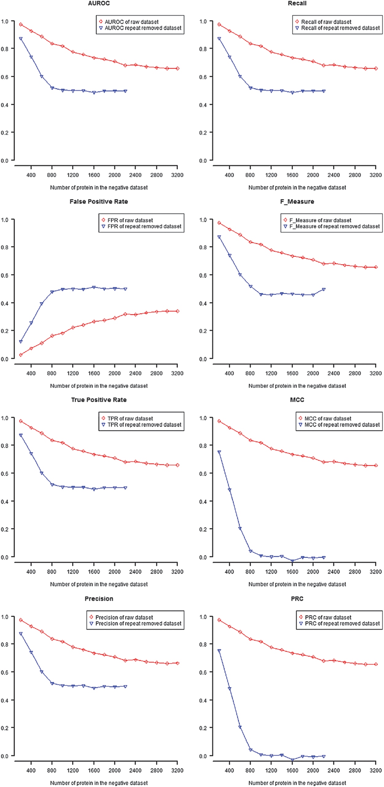
Performances of prediction in auto covariance model. TPR, FPR, precision, recall, F-measure, MCC, AUROC, and AUPRC were used to evaluate the performances of predictions of the original dataset and the repeat-protein removed dataset.

3.3. Performances of prediction decrease as protein repetitiveness and protein repeat rate decrease

Protein repetitiveness were varied in different negative datasets. The relationship between performances of prediction and protein repetitiveness of PPI datasets were evaluated by correlation analysis. Significant correlation between all performances of prediction and protein repetitiveness of the PPI dataset were shown (Table 3 and Supplemental Table). TPR, precision, recall, F-measure, MCC, AUROC, and AUPRC showed positive correlation and, on the other hand, FPR showed negative correlation in all models, species, and both in raw dataset and repeat-protein removed datasets (Tables 3, and 4, and Supplementary Tables 1–22). This showed that protein repetitiveness might affected performances of prediction no matter in the original positive dataset or in the repeat-protein removed positive dataset.

Table 3.

Pearson Correlation Analysis of Performance (AC Model) and Protein Repeat Number and Repeat Rate in Original Dataset of H. sapiens

Performance measurement	Repeat rate correlation	Repeat rate p-value	Repeat number correlation	Repeat number p-value
ROC	0.87	1.06E-05	0.96	4.84E-09
PRC	0.90	1.68E-06	0.94	1.05E-07
MCC	0.87	9.86E-06	0.96	6.42E-09
F_Measure	0.87	1.16E-05	0.96	3.62E-09
Recall	0.87	1.06E-05	0.96	4.84E-09
Precision	0.87	9.25E-06	0.96	8.47E-09
TPR	0.87	1.06E-05	0.96	4.84E-09
FPR	−0.87	1.06E-05	−0.96	4.84E-09

Table 4.

Pearson Correlation Analysis of Performance (AC Model) and Protein Repeat Number and Repeat Rate in the Repeat Removed Dataset of H. sapiens

Performance measurement	Repeat rate correlation	Repeat rate p-value	Repeat number correlation	Repeat number p-value
ROC	0.97	5.33E-07	0.83	0.001
PRC	0.98	4.71E-08	0.80	0.003
MCC	0.97	4.75E-07	0.84	0.001
F_Measure	0.96	2.26E-06	0.84	0.001
Recall	0.97	5.33E-07	0.83	0.001
Precision	0.97	4.76E-07	0.84	0.001
TPR	0.97	5.33E-07	0.83	0.001
FPR	−0.97	5.33E-07	−0.83	0.001

3.4. Distributions of repeated proteins in final datasets

In Table 5 and Table 6, we show parts of the degree distribution of raw dataset graphs and repeat-protein removed dataset graphs of H. sapiens, respectively. The maximum degrees of raw dataset graphs listed in Table 5 were from 180 to 200, while those of repeat-protein removed graphs in Table 6 were from 3 to 19. The low maximum degree of hub proteins in repeat-protein removed graphs showed that our repeat removing algorithm tended to remove hub proteins. The high maximum degree of hub proteins in raw dataset graphs lead to high repeat number and high repeat rate and this may contribute effect to high prediction performance in raw datasets (Table 5 and Fig. 1 red lines). In addition, although maximum degree of hub proteins were relatively low in repeat-protein removed dataset graphs, they also lead to high repeat number and high repeat rate due to large amounts of proteins with degree greater than 1 (Table 6). This implied that the presence of hub proteins or large amounts of proteins with relatively low degree in a dataset may both lead to in high prediction performance.

Table 5.

Degree Distributions of the Raw Dataset Graphs of H. sapiens

Datasets
(H, NH₂₀₀)
degree	1	2	3	4	5	6	7	8	9	10	11	12	13
number of vertices (proteins)	1467	630	314	195	117	81	53	51	37	34	22	9	13
degree	14	15	16	17	18	19	20	21	22	23	24	25	26
number of vertices (proteins)	12	5	6	51	5	6	3	2	5	4	5	3	4
degree	27	28	29	30	31	32	33	34	35	36	37	38	39
number of vertices (proteins)	5	4	8	7	7	6	15	9	2	9	5	7	3
degree	40	41	43	45	46	47	49	50	54	55	56	57	58
number of vertices (proteins)	5	2	3	1	2	1	1	1	1	1	1	2	3
degree	59	60	61	63	64	65	67	68	69	71	72	73	74
number of vertices (proteins)	1	1	4	2	1	1	1	1	1	5	2	5	5
degree	75	76	77	78	79	80	82	83	101	200
number of vertices (proteins)	14	8	4	6	6	1	4	1	1	1
(H, NH₈₀₀)
degree	1	2	3	4	5	6	7	8	9	10	11	12	13
number of vertices (proteins)	1170	509	256	164	102	92	63	79	72	95	64	59	62
degree	14	15	16	17	18	19	20	21	22	23	24	25	26
number of vertices (proteins)	57	44	42	46	96	122	30	14	11	9	5	2	1
degree	27	28	30	33	34	43	79	180
number of vertices (proteins)	3	4	1	1	1	1	1	1
(H, NH₁₄₀₀)
degree	1	2	3	4	5	6	7	8	9	10	11	12	13
number of vertices (proteins)	886	387	24	177	163	161	144	164	144	149	357	111	56
degree	14	15	16	17	18	19	20	21	22	23	24	25	26
number of vertices (proteins)	38	21	18	7	12	11	10	4	5	1	1	1	2
degree	27	28	32	36	45	80	180
number of vertices (proteins)	1	2	1	1	1	1	1
(H, NH₂₀₀₀)
degree	1	2	3	4	5	6	7	8	9	10	11	12	13
number of vertices (proteins)	610	310	237	251	238	284	310	388	279	132	70	39	25
degree	14	15	16	17	18	19	20	21	22	23	24	25	26
number of vertices (proteins)	20	17	13	16	7	7	4	3	2	4	1	1	2
degree	27	28	31	33	34	43	81	183
number of vertices (proteins)	1	1	2	1	1	1	1	1
(H, NH₂₆₀₀)
degree	1	2	3	4	5	6	7	8	9	10	11	12	13
number of vertices (proteins)	320	253	274	337	440	565	504	196	119	65	61	27	20
degree	14	15	16	17	18	19	20	21	22	23	25	26	27
number of vertices (proteins)	23	16	13	8	9	3	4	3	2	5	2	1	2
degree	30	33	35	43	82	181
number of vertices (proteins)	1	2	1	1	1	1
(H, NH₃₂₀₀)
degree	1	2	3	4	5	6	7	8	9	10	11	12	13
number of vertices (proteins)	68	189	386	466	839	576	261	143	106	55	47	35	20
degree	14	15	16	17	18	19	20	21	22	23	24	25	28
number of vertices (proteins)	16	12	14	6	4	6	6	4	5	2	2	2	3
degree	31	34	35	43	79	181
number of vertices (proteins)	1	1	1	1	1	1

Table 6.

Degree Distribution of the Repeat-Protein Removed Dataset Graphs of H. sapiens

Datasets
(H_M, XH₂₀₀)
Degree	1	3	4	5	6	7	8	9	10
number of vertices (proteins)	2098	1	2	6	10	12	20	18	15
Degree	11	12	13	14	15	16	17	18	19
number of vertices (proteins)	11	8	4	5	13	15	23	27	10
(H_M, XH₆₀₀)
degree	1	2	3	4	5	6	7
number of vertices (proteins)	1718	40	89	102	106	108	135
(H_M, XH₁₀₀₀)
degree	1	2	3	4	5
number of vertices (proteins)	1372	205	249	293	179
(H_M, XH₁₄₀₀)
degree	1	2	3	4	5
number of vertices (proteins)	1073	374	646	188	17
(H_M, XH₁₈₀₀)
degree	1	2	3
number of vertices (proteins)	822	654	822
(H_M, XH₂₂₀₀)
degree	1	2	3
number of vertices (proteins)	666	966	666

Discussion

In this study, the relationships between protein repetitiveness and performances of prediction of three SVM models were examined in H. sapiens and S.cerevisiae, respectively. We showed that removing repeated proteins in the positive or negative dataset would decrease performance of prediction dramatically, and performances of prediction increase with increasing protein repetitiveness of the negative dataset. Although we only investigated this relationship in SVM models with limited data, results might show a hint or a possibility that protein repetitiveness of the dataset is a bias factor of prediction performance. One possible reason for this phenomenon is the following: each vector in an encoding data of a dataset, other than label, is the concatenation of two vectors transformed from protein sequences of a protein pair. If repeat proteins in the dataset, they would create more duplicated vectors and the SVM predictor will learn from this repeated pattern as the same result. As a consequence, this might lead to high prediction performances of the SVM-based prediction methods because the positive and negative datasets might contain certain degree of repeat proteins.

In the previous studies, Yu et al. (2010) mentioned that the presence of ‘hub’ proteins that interact with many other proteins in the positive dataset leads to a strong bias that invalidates most performance estimates. We show that even removing those hub proteins in the positive dataset, such bias still contribute effects to performance due to protein repetitiveness of the negative dataset. Ben-Hur and Noble (2006) mentioned that restricting negative examples to non-colocalized protein pairs leads to a biased estimate of the accuracy of a predictor of protein–protein interactions and biased distribution of negative examples leads to over-optimistic estimates of classifier accuracy. In this study, we further show that the presence of hub proteins or large amounts of proteins with relatively low degree in a dataset may both lead to high prediction performance.

Although we only analyzed the relationship between protein repetitiveness and performances of PPI prediction, the results might be applied to other kinds of predictions such as gene–protein interactions, RNA–protein interactions, gene–gene interactions, gene–disease interactions, RNA–disease interactions, protein–DNA interactions, drug–protein interactions, and cell–cell interactions (Cheng et al., 2015; Koo et al., 2013; McKinney et al., 2006; Muppiral et al., 2011; Piro and Di Cunto, 2012; Rao et al., 2014; Westra et al., 2007; Xu et al., 2015; Zhang et al., 2014; Zou et al., 2013). The most similar characteristic between these predictions and PPI prediction was object repetitiveness. As a consequence, performances of SVM prediction might be also affected by repetitiveness in the positive dataset or negative dataset.

In this study, we only conducted SVM on PPI prediction and analyzed the effect of protein repetitiveness on performances. The mechanism of these effects on performances of SVM prediction is still not clear. Improvement or modification of the SVM algorithm to avoid the effect of repetitiveness on performances of prediction is still worthy of future investigation.

Footnotes

Author Disclosure Statement

No competing financial interests exist.

References

Alberts

1998. The cell as a collection of protein machines: Preparing the next generation of molecular biologists. Cell, 92, 291–294.

Aranda

, Achuthan

, Alam-Faruque

, et al. 2002. The IntAct molecular interaction database in 2010. Nucleic Acids Res., 2010, 38, D525–D531.

Auerbach

, Thaminy

, Hottiger

M.O.

, and Stagljar

The post-genomic era of interactive proteomics: Facts and perspectives. Proteomics, 2, 611–623.

Barabasi

A.L.

, and Oltvai

Z.N.

2004. Network biology: Understanding the cell's functional organization. Nature Rev. Genetics, 5, 101–113.

Bauer

, and Kuster

2003. Affinity purification-mass spectrometry. Eur. J. Biochem., 270, 570–578.

Ben-Hur

, and Noble

2006. Choosing negative examples for the prediction of protein-protein interactions. BMC Bioinformatics. 7, S2.

Ceol

, Chatr Aryamontri

, Licata

, et al. 2010. MINT, the molecular interaction database: 2009 update. Nucleic Acids Res. 38, D532–D539.

Cheng

, Zhou

, and Guan

2015. Computationally predicting protein-RNA interactions using only positive and unlabeled examples. J. Bioinformat. Comput. Biol. 13, 1541005.

Fawcett

2006. An introduction to ROC analysis. Pattern Recog. Lett., 27, 861–874.

10.

Guan

, and Kiss-Toth

2008. Advanced technologies for studies on protein interactomes, In: Werther

, Seitz

, eds. Protein–Protein Interaction, 1–24. Springer Berlin Heidelberg.

11.

Guo

, Yu

, Wen

, et al. 2008. Using support vector machine combined with auto covariance to predict protein–protein interactions from protein sequences. Nucleic Acids Res. 36, 3025–3030.

12.

Hall

, Frank

, Holmes

, et al. 2009. The WEKA data mining software: An update. ACM SIGKDD Explorations Newslett. 11, 10–18.

13.

Hart

G.T.

, Ramani

, and Marcotte

2006. How complete are current yeast and human protein-interaction networks?. Genome Biol. 7, 120.

14.

Ito

, Chiba

, Ozawa

, et al. 2001. A comprehensive two-hybrid analysis to explore the yeast protein interactome. Proc. Natl. Acad. Sci. USA., 98, 4569–4574.

15.

Jansen

, Yu

, Greenbaum

, et al. 2003. A Bayesian networks approach for predicting protein-protein interactions from genomic data. Science, 302, 449–453.

16.

Keshava Prasad

T.S.

, Goel

, Kandasamy

, et al. 2009. Human Protein Reference Database–2009 update. Nucleic Acids Res. 37, D767–D772.

17.

Koo

C.L.

, Liew

M.J.

, Mohamad

M.S.

, et al. 2013. A review for detecting gene-gene interactions using machine learning methods in genetic epidemiology. BioMed. Res. Intl. 2013, 13.

18.

McKinney

B.A.

, Reif

D.M.

, Ritchie

M.D.

, et al. 2006. Machine learning for detecting gene-gene interactions: A review. Appl. Bioinformat., 5, 77–88.

19.

Michnick

S.W.

, MacDonald

M.L.

, and Westwick

J.K.

2006. Chemical genetic strategies to delineate MAP kinase signaling pathways using protein-fragment complementation assays (PCA). Methods, 40, 287–293.

20.

Mosca

, Pons

, Céol

, et al. 2013. Towards a detailed atlas of protein–protein interactions. Curr. Opin. Struct. Biol., 23, 929–940.

21.

Muppirala

U.K.

, Honavar

V.G.

, and Dobbs

2011. Predicting RNA-protein interactions using only sequence information. BMC Bioinformat. 12, 489.

22.

Piro

R.M.

, and Di Cunto

2012. Computational approaches to disease-gene prediction: Rationale, classification and successes. FEBS J. 279, 678–696.

23.

Ramani

A.K.

, and Marcotte

E.M.

2003. Exploiting the co-evolution of interacting proteins to discover interaction specificity. J. Mol. Biol., 327, 273–284.

24.

Rao

V.S.

, Srinivas

, Sujini

G.N.

, et al. 2014. Protein-protein interaction detection: Methods and analysis. Intl. J. Proteom. 2014, 12.

25.

Rhodes

D.R.

, Tomlins

S.A.

, Varambally

, et al. 2005. Probabilistic model of the human protein-protein interaction network. Nature Biotechnol. 23, 951–959.

26.

Salwinski

, Miller

C.S.

, Smith

A.J.

, et al. 2004. The Database of Interacting Proteins: 2004 update. Nucleic Acids Res. 32, D449–D451.

27.

Scott

, and Barton

2007. Probabilistic prediction and ranking of human protein-protein interactions. BMC Bioinformat. 8, 239.

28.

Shen

, Zhang

, Luo

, et al. 2007. Predicting protein–protein interactions based only on sequences information. Proc. Natl. Acad. Sci., 104, 4337–4341.

29.

Shoemaker

B.A.

, and Panchenko

A.R.

2007. Deciphering protein–protein interactions. Part II. Computational methods to predict protein and domain interaction partners. PloS Comput. Biol. 3, e43.

30.

Stark

, Breitkreutz

B.J.

, Reguly

, et al. 2006. BioGRID: A general repository for interaction datasets. Nucleic Acids Res. 34, D535–D539.

31.

Trabuco

L.G.

, Betts

M.J.

, and Russell

R.B.

2012. Negative protein–protein interaction datasets derived from large-scale two-hybrid experiments. Methods, 58, 343–348.

32.

Uetz

, Giot

, Cagney

, et al. 2000. A comprehensive analysis of protein-protein interactions in Saccharomyces cerevisiae. Nature, 403, 623–627.

33.

Walhout

A.J.

, and Vidal

2001. Protein interaction maps for model organisms. Nature Rev Mol Cell Biol. 2, 55–63.

34.

Westra

R.L.

, Hollanders

, Jan Bex

, et al. The identification of dynamic gene-protein networks. In: Knowledge, Discovery and Emergent Complexity in Bioinformatics, 157–170. In: Tuyls

, Westra

, Saeys

, et al., eds. Springer Berlin Heidelberg.

35.

, Zhou

, Wang

, et al. 2015. Identifying DNA-binding proteins by combining support vector machine and PSSM distance transformation. BMC Syst. Biol. 9, S10.

36.

Yang

, Xia

J.F.

, and Gui

2010. Prediction of protein-protein interactions from protein sequence using local descriptors. Protein Peptide Lett. 17, 1085–1090.

37.

, and Dong

2003. Computational analyses of high-throughput protein-protein interaction data. Curr. Protein Peptide Sci., 4, 159–180.

38.

, Guo

, Needham

C.J.

, et al. 2010. Simple sequence-based kernels do not predict protein–protein interactions. Bioinformatics, 26, 2610–2614.

39.

Zhang

S.W.

, Hao

L.Y.

, and Zhang

T.H.

2014. Prediction of protein–protein interaction with pairwise kernel support vector machine. Intl. J. Mol. Sci. 15, 3220.

40.

Zou

, Gong

, and Li

2013. An improved sequence based prediction protocol for DNA-binding proteins using SVM and comprehensive feature analysis. BMC Bioinformat. 14, 90.

Supplementary Material

Please find the following supplemental material available below.

For Open Access articles published under a Creative Commons License, all supplemental material carries the same license as the article it is associated with.

For non-Open Access articles published, all supplemental material carries a non-exclusive license, and permission requests for re-use of supplemental material or any part of supplemental material shall be sent directly to the copyright owner as specified in the copyright notice associated with the article.

0.00 MB

0.03 MB

0.63 MB

1.27 MB

1.25 MB

0.23 MB

0.18 MB

0.02 MB