A Provably Efficient Algorithm for the k -Mismatch Average Common Substring Problem

1. Introduction

Treating biosequences as “documents of evolution” (Zuckerkandl and Pauling, 1965) is one of the oldest ideas of molecular biology. In this vein, measures of sequence similarity and distance primarily emerged in coding theory have provided the natural backbone in the development of tools for deriving taxonomies and phylogenies from systematic biosequence comparison. Beginning with Fitch and Margoliash (Fitch et al., 1967), the established methods for automated inference of phylogeny have been based on sequence alignment of protein orthologues or their genes, tRNAs, 16S rRNAs, 23S rRNAs, etc. In 1994, the DIMACS special year on computational biology devoted one of its four main workshops to sequence comparison. By the end of which, more than 1200 noteworthy publications were counted on this subject (Apostolico and Giancarlo, 1998).

In subsequent years, the context has drastically evolved from the original condition of scarcity of data, and a plethora of new problems have emerged. To begin with, dithering the parameters involved in alignment proved not a simple task. Common orthologues are difficult to identify for prokaryotes due to their wide genetic diversity. Lateral transfer of proteins may lead to completely wrong results, for example the entire ribosomal operon (5S + 16S + 23S) in E. coli may be artificially replaced by that from other species (Asai et al., 1999). The resulting trees are prone to intrinsic biases brought about by the specific data being analyzed and so on. To summarize, classical alignment distances become both computationally expensive and scarcely significant when they are applied to entire genomes and are being complemented or even entirely supplanted by global (algebraic) similarity measures that refer, implicitly or explicitly, to the subword composition of sequences, sometimes collectively referred to as “alignment-free” comparisons (see, e.g., Apostolico and Cunial, 2011; Apostolico and Denas, 2008; Apostolico et al., 2010; Blaisdell, 1986; Clift et al., 1986; Cunial and Apostolico, 2012; Edgar, 2004; Ferragina et al., 2007; Gatlin, 1972; Hao and Qi, 2004; Höhl and Ragan, 2007; Höhl et al., 2006; Li et al., 2004; Morgenstern et al., 2014; Otu and Sayood, 2003; Qi et al., 2004; Ulitsky et al., 2006; Van Helden, 2004; Vinga and Almeida, 2003; Wu et al., 1997).

The average common substring measure proposed by Burstein et al. and Ulitsky et al. (Burstein et al., 2005; Ulitsky et al., 2006) is a simple alignment-free sequence comparison method that nevertheless achieved high accuracy in large-scale phylogenetic reconstruction. Formally, let X and Y denote two sequences over the alphabet Σ. We use the notation |X| to denote the length of X, X[i] (1 ≤ i ≤|X|) to denote its ith leftmost character, and X[i…j] to denote the substring X[i]X[i + 1]…X[j]. Let X _i denote the suffix of X starting at i^th position, that is, X _i  = X[i…|X|]. Let \documentclass{aastex}\usepackage{amsbsy}\usepackage{amsfonts}\usepackage{amssymb}\usepackage{bm}\usepackage{mathrsfs}\usepackage{pifont}\usepackage{stmaryrd}\usepackage{textcomp}\usepackage{portland, xspace}\usepackage{amsmath, amsxtra}\pagestyle{empty}\DeclareMathSizes{10}{9}{7}{6}\begin{document} \begin{align*} \lambda ({\sf X}_i , { \sf Y} ) = \max\limits_{1 \leq j \leq \mid { \sf Y} \mid} \mid {\sf LCP} ({\sf X}_i ,{\sf Y}_j ) \mid , \end{align*} \end{document}

where LCP(X _i , Y _j ) denote the longest common prefix between suffixes X _i and Y _j . The average common substring, ACS(X, Y), is defined as: \documentclass{aastex}\usepackage{amsbsy}\usepackage{amsfonts}\usepackage{amssymb}\usepackage{bm}\usepackage{mathrsfs}\usepackage{pifont}\usepackage{stmaryrd}\usepackage{textcomp}\usepackage{portland, xspace}\usepackage{amsmath, amsxtra}\pagestyle{empty}\DeclareMathSizes{10}{9}{7}{6}\begin{document} \begin{align*} { \sf ACS } ( { \sf X } , { \sf Y } ) = \frac { 1 } { \mid { \sf X } \mid } \mathop \sum \limits_ { i = 1 } ^ { \mid { \sf X } \mid } \lambda ( { \sf X } _i , { \sf Y } )\end{align*} \end{document}

Therefore, ACS(X, Y) is the average of the length of the longest prefix of a suffix of X occurring in Y. One then takes ACS(X, Y) / log |Y| to normalize with respect to the length of Y. A distance metric based on ACS (Ulitsky et al., 2006) is obtained by first taking the inverse of the similarity measure ACS(X, Y) / log |Y| and then subtracting a term to guarantee the condition Dist(X, X) = 0. Specifically, this yields \documentclass{aastex}\usepackage{amsbsy}\usepackage{amsfonts}\usepackage{amssymb}\usepackage{bm}\usepackage{mathrsfs}\usepackage{pifont}\usepackage{stmaryrd}\usepackage{textcomp}\usepackage{portland, xspace}\usepackage{amsmath, amsxtra}\pagestyle{empty}\DeclareMathSizes{10}{9}{7}{6}\begin{document} \begin{align*} { \sf Dist } ^ { \prime } ( { \sf X } , { \sf Y } ) = \frac { \log \mid { \sf Y } \mid } { { \sf ACS } ( { \sf X } , { \sf Y } ) } - \frac { \log \mid { \sf X } \mid } { { \sf ACS } ( { \sf X } , { \sf X } ) } \end{align*} \end{document}

where the correction term log |X|/ACS(X, X) = 2log |X|/|X| vanishes as |X|→∞. Following this, one compensates for symmetry by taking \documentclass{aastex}\usepackage{amsbsy}\usepackage{amsfonts}\usepackage{amssymb}\usepackage{bm}\usepackage{mathrsfs}\usepackage{pifont}\usepackage{stmaryrd}\usepackage{textcomp}\usepackage{portland, xspace}\usepackage{amsmath, amsxtra}\pagestyle{empty}\DeclareMathSizes{10}{9}{7}{6}\begin{document} \begin{align*} { \sf Dist } ( { \sf X } , { \sf Y } ) = \frac { { \sf Dist } ^ { \prime } ( { \sf X } , { \sf Y } ) + { \sf Dist } ^ { \prime } ( { \sf Y } , { \sf X } ) } { 2 } \end{align*} \end{document}

as the final distance. We can easily compute ACS (and then Dist′ and Dist) using a (generalized) suffix tree–based algorithm in time and space linear in the total length of X and Y.

Since its introduction, the ACS measure has gained considerable attention (Apostolico, 2010; Bonham-Carter et al., 2013; Chang and Wang, 2011; Comin et al., 2012; Domazet-Lošo and Haubold, 2009; Fracasso, 2014; Guyon et al., 2009). An important direction of research is to improve the measure by allowing a bounded number k of mismatches in sequence comparison. Define λ_k(X _i , Y) as: \documentclass{aastex}\usepackage{amsbsy}\usepackage{amsfonts}\usepackage{amssymb}\usepackage{bm}\usepackage{mathrsfs}\usepackage{pifont}\usepackage{stmaryrd}\usepackage{textcomp}\usepackage{portland, xspace}\usepackage{amsmath, amsxtra}\pagestyle{empty}\DeclareMathSizes{10}{9}{7}{6}\begin{document} \begin{align*}\lambda_k ( { \sf X}_i , { \sf Y} ) = \max \limits_{1 \leq j \leq \mid { \sf Y} \mid} \mid { \sf LCP}_k ( { \sf X}_i , { \sf Y}_j ) \mid ,\end{align*} \end{document}

where LCP _k (X _i , Y _j ) denotes the longest common prefix between suffixes X _i and Y _j with allowance for up to k mismatches. The k-mismatch average common substring of X and Y, denoted ACS _k (X, Y), is defined as: \documentclass{aastex}\usepackage{amsbsy}\usepackage{amsfonts}\usepackage{amssymb}\usepackage{bm}\usepackage{mathrsfs}\usepackage{pifont}\usepackage{stmaryrd}\usepackage{textcomp}\usepackage{portland, xspace}\usepackage{amsmath, amsxtra}\pagestyle{empty}\DeclareMathSizes{10}{9}{7}{6}\begin{document} \begin{align*} { \sf ACS } _k ( { \sf X } , { \sf Y } ) = \frac { 1 } { \mid { \sf X } \mid } \mathop \sum \limits_ { i = 1 } ^ { \mid { \sf X } \mid } \lambda_k ( { \sf X } _i , { \sf Y } )\end{align*} \end{document}

An algorithm quite recently proposed by Leimeister and Morgenstern (2014) for computing ACS _k (X, Y) requires O(|X|×|Y|×k) worst-case run-time, which is quadratic when |X| and |Y| are of the same order, even for k = 1 (also see Pizzi, 2015). However, it is amply documented in Horwege et al. (2014) and Leimeister and Morgenstern (2014) that the ACS _k (X, Y) paradigm does yield better phylogenetic classification than both the exact version of the problem and classical approaches using multiple sequence alignment and maximum likelihood. Although Leimeister and Morgenstern (2014) (also see the recent work by Thankachan et al., 2015) proposed faster heuristics to approximate ACS _k , designing a provably efficient algorithm remained open. Our goal in this work is to compute ACS _k (X, Y) (hence also the naturally associated Dist _k (X, Y)) in time and space that is as close to linear in n = |X| + |Y| as possible. Our main contribution is summarized in the following theorem:

Theorem 1 Let X and Y be two sequences of n characters in total. Let X _i be the suffix of X starting at location i, and λ_k(X _i , Y) be the length of the longest prefix of X _i that appears in Y with at most k mismatches. Then λ_k(X _i , Y) can be computed for all values of i in O(n log ^k n) overall time using O(n) working space for any constant k.

Using Theorem 1, we can compute ACS _k (X, Y) in O(n log^kn) time. As a byproduct, we also improved upon the best-known results for the k-mismatch longest common substring problem (LCS _k ), which previously took linear space and O(n log n) time for k = 1, but takes almost quadratic time otherwise (Babenko and Starikovskaya, 2008; Flouri et al., 2015; Grabowski, 2015). Notice that LCS _k (X, Y) is the substring corresponding to max{λ_k(X _i , Y) ∣1 ≤ i ≤ |X|}, hence it can be computed within the same space-time complexity of Theorem 1.

Theorem 2 (k-mismatch longest common substring) Given two sequences of total length n, their longest common substring with at most k mismatches can be computed in O(n log ^k  n) time using O(n) space for any constant k.

2. Key Concepts and Properties

A generalized suffix tree of X and Y (from now onward called GST) is a compact trie that stores all (nonempty) suffixes of X and Y. It takes O(n) space and can be constructed in O(n) space and time (McCreight, 1976; Weiner, 1973), where n = |X| + |Y|. Using GST, we can compute |LCP(X _i , Y _j )| for any (i, j) pair in constant time. Specifically, |LCP(X _i , Y _j )| is the string depth of the lowest common ancestor (LCA) of leaves representing suffixes X _i and Y _j in the GST. Then, |LCP _k (X _i , Y _j )| for any (i, j) pair can be computed in O(k) time using the following recursion. \documentclass{aastex}\usepackage{amsbsy}\usepackage{amsfonts}\usepackage{amssymb}\usepackage{bm}\usepackage{mathrsfs}\usepackage{pifont}\usepackage{stmaryrd}\usepackage{textcomp}\usepackage{portland, xspace}\usepackage{amsmath, amsxtra}\pagestyle{empty}\DeclareMathSizes{10}{9}{7}{6}\begin{document} \begin{align*}\mid { \sf LCP}_k ( { \sf X}_i , { \sf Y}_j ) \mid = \begin{cases}z , { \rm where} \ z = \mid { \sf LCP} ( { \sf X}_i , { \sf Y}_j ) \mid \quad \quad \quad \quad { \rm if} \ k = 0 \\ z + 1 + \mid { \sf LCP}_{k - 1} ( { \sf X}_{i + z + 1} , { \sf Y}_{j + z + 1} ) \mid \; \quad { \rm if} \ k > 0\end{cases}\end{align*} \end{document}

Therefore, ACS _k (·,·) can be computed in O(n²k) time. Clearly, this approach is computationally expensive. To describe our faster approach, we first introduce some definitions and prove resulting useful properties. Throughout this article, we treat k as a constant.

3. An Overview of Our Algorithm

Definition 3 For a fixed k, a universe (denoted by \documentclass{aastex}\usepackage{amsbsy}\usepackage{amsfonts}\usepackage{amssymb}\usepackage{bm}\usepackage{mathrsfs}\usepackage{pifont}\usepackage{stmaryrd}\usepackage{textcomp}\usepackage{portland, xspace}\usepackage{amsmath, amsxtra}\pagestyle{empty}\DeclareMathSizes{10}{9}{7}{6}\begin{document} $${ \cal U}$$ \end{document} ) is a set of modified suffixes, such that for any 1 ≤ i ≤ |X| and 1 ≤ j ≤ |Y|, \documentclass{aastex}\usepackage{amsbsy}\usepackage{amsfonts}\usepackage{amssymb}\usepackage{bm}\usepackage{mathrsfs}\usepackage{pifont}\usepackage{stmaryrd}\usepackage{textcomp}\usepackage{portland, xspace}\usepackage{amsmath, amsxtra}\pagestyle{empty}\DeclareMathSizes{10}{9}{7}{6}\begin{document} $${ \cal U}$$ \end{document} contains two modified suffixes that together form an (i, j) _k -maxpair. A partition of \documentclass{aastex}\usepackage{amsbsy}\usepackage{amsfonts}\usepackage{amssymb}\usepackage{bm}\usepackage{mathrsfs}\usepackage{pifont}\usepackage{stmaryrd}\usepackage{textcomp}\usepackage{portland, xspace}\usepackage{amsmath, amsxtra}\pagestyle{empty}\DeclareMathSizes{10}{9}{7}{6}\begin{document} $${ \cal U}$$ \end{document} is a collection of its subsets \documentclass{aastex}\usepackage{amsbsy}\usepackage{amsfonts}\usepackage{amssymb}\usepackage{bm}\usepackage{mathrsfs}\usepackage{pifont}\usepackage{stmaryrd}\usepackage{textcomp}\usepackage{portland, xspace}\usepackage{amsmath, amsxtra}\pagestyle{empty}\DeclareMathSizes{10}{9}{7}{6}\begin{document} $${ \cal P}_1 , { \cal P}_2 , \ldots , { \cal P}_t$$ \end{document} such that ∀i, j, ∃ an (i, j) _k -maxpair in at least one \documentclass{aastex}\usepackage{amsbsy}\usepackage{amsfonts}\usepackage{amssymb}\usepackage{bm}\usepackage{mathrsfs}\usepackage{pifont}\usepackage{stmaryrd}\usepackage{textcomp}\usepackage{portland, xspace}\usepackage{amsmath, amsxtra}\pagestyle{empty}\DeclareMathSizes{10}{9}{7}{6}\begin{document} $${ \cal P}_f , 1 \leq f \leq t$$ \end{document} .

The key intuition behind our algorithm is that by processing a given \documentclass{aastex}\usepackage{amsbsy}\usepackage{amsfonts}\usepackage{amssymb}\usepackage{bm}\usepackage{mathrsfs}\usepackage{pifont}\usepackage{stmaryrd}\usepackage{textcomp}\usepackage{portland, xspace}\usepackage{amsmath, amsxtra}\pagestyle{empty}\DeclareMathSizes{10}{9}{7}{6}\begin{document} $${ \cal U}$$ \end{document} in time and space linear (or near-linear) to its size, we can compute ACS _k . Partitioning \documentclass{aastex}\usepackage{amsbsy}\usepackage{amsfonts}\usepackage{amssymb}\usepackage{bm}\usepackage{mathrsfs}\usepackage{pifont}\usepackage{stmaryrd}\usepackage{textcomp}\usepackage{portland, xspace}\usepackage{amsmath, amsxtra}\pagestyle{empty}\DeclareMathSizes{10}{9}{7}{6}\begin{document} $${ \cal U}$$ \end{document} provides a more convenient way to compute ACS _k by splitting the potentially large \documentclass{aastex}\usepackage{amsbsy}\usepackage{amsfonts}\usepackage{amssymb}\usepackage{bm}\usepackage{mathrsfs}\usepackage{pifont}\usepackage{stmaryrd}\usepackage{textcomp}\usepackage{portland, xspace}\usepackage{amsmath, amsxtra}\pagestyle{empty}\DeclareMathSizes{10}{9}{7}{6}\begin{document} $${ \cal U}$$ \end{document} into multiple smaller sets and processing them independently. Clearly, there exists a universe of size O(n²). However, our algorithm is based on the existence of a partition as summarized in the following lemma.

Lemma 3 There exists a universe \documentclass{aastex}\usepackage{amsbsy}\usepackage{amsfonts}\usepackage{amssymb}\usepackage{bm}\usepackage{mathrsfs}\usepackage{pifont}\usepackage{stmaryrd}\usepackage{textcomp}\usepackage{portland, xspace}\usepackage{amsmath, amsxtra}\pagestyle{empty}\DeclareMathSizes{10}{9}{7}{6}\begin{document} $${ \cal U}$$ \end{document} and its partition \documentclass{aastex}\usepackage{amsbsy}\usepackage{amsfonts}\usepackage{amssymb}\usepackage{bm}\usepackage{mathrsfs}\usepackage{pifont}\usepackage{stmaryrd}\usepackage{textcomp}\usepackage{portland, xspace}\usepackage{amsmath, amsxtra}\pagestyle{empty}\DeclareMathSizes{10}{9}{7}{6}\begin{document} $$\{ { \cal P}_1 , { \cal P}_2 , \ldots , { \cal P}_t \} $$ \end{document} , such that \documentclass{aastex}\usepackage{amsbsy}\usepackage{amsfonts}\usepackage{amssymb}\usepackage{bm}\usepackage{mathrsfs}\usepackage{pifont}\usepackage{stmaryrd}\usepackage{textcomp}\usepackage{portland, xspace}\usepackage{amsmath, amsxtra}\pagestyle{empty}\DeclareMathSizes{10}{9}{7}{6}\begin{document} \begin{align*}\max \limits_{1 \leq f \leq t} \mid { \cal P}_f \mid = O ( n ) \ \ { \rm and} \ \ \sum \limits_{1 \leq f \leq t} \mid { \cal P}_f \mid = O ( n \log^k n )\end{align*} \end{document}

Our algorithm can be viewed as consisting of two phases. In the first phase, we generate members of the partition, one at a time. The second phase takes each member \documentclass{aastex}\usepackage{amsbsy}\usepackage{amsfonts}\usepackage{amssymb}\usepackage{bm}\usepackage{mathrsfs}\usepackage{pifont}\usepackage{stmaryrd}\usepackage{textcomp}\usepackage{portland, xspace}\usepackage{amsmath, amsxtra}\pagestyle{empty}\DeclareMathSizes{10}{9}{7}{6}\begin{document} $${ \cal P}_f$$ \end{document} separately and extracts information necessary for computing ACS _k . We show that using O(n) working space, members can be generated one after the other in overall O(n log ^k  n) time. Similarly, using O(n) working space, members can be processed one after the other in overall O(n log ^k  n) time. Therefore, by interleaving phase 1 and phase 2 (i.e., as soon as a member is generated, process it and then discard it from the working space), we achieve the space–time complexities in Theorem 1. We now present the phases in detail.

4. Phase 1: Constructing the Partition

Our method for constructing the partition borrows from ideas in Cole et al. (2004) on string indexing for approximate pattern-matching queries, which itself relies on the classic heavy path decomposition strategy invented by Sleator and Tarjan (1981). The procedure is recursive, which can be best explained as constructing a tree (TREE) as follows:

Definition 4 TREE is of depth k and each node x in TREE is associated with a set \documentclass{aastex}\usepackage{amsbsy}\usepackage{amsfonts}\usepackage{amssymb}\usepackage{bm}\usepackage{mathrsfs}\usepackage{pifont}\usepackage{stmaryrd}\usepackage{textcomp}\usepackage{portland, xspace}\usepackage{amsmath, amsxtra}\pagestyle{empty}\DeclareMathSizes{10}{9}{7}{6}\begin{document} $${ \cal S}_x$$ \end{document} of modified suffixes. The set associated with root consists of all n suffixes of X and Y. Then, starting with x = root, the sets associated with the children of any internal node x are generated from \documentclass{aastex}\usepackage{amsbsy}\usepackage{amsfonts}\usepackage{amssymb}\usepackage{bm}\usepackage{mathrsfs}\usepackage{pifont}\usepackage{stmaryrd}\usepackage{textcomp}\usepackage{portland, xspace}\usepackage{amsmath, amsxtra}\pagestyle{empty}\DeclareMathSizes{10}{9}{7}{6}\begin{document} $${ \cal S}_x$$ \end{document} using a recursive procedure maintaining the following properties:

1. The size of the set associated with any child node of x is \documentclass{aastex}\usepackage{amsbsy}\usepackage{amsfonts}\usepackage{amssymb}\usepackage{bm}\usepackage{mathrsfs}\usepackage{pifont}\usepackage{stmaryrd}\usepackage{textcomp}\usepackage{portland, xspace}\usepackage{amsmath, amsxtra}\pagestyle{empty}\DeclareMathSizes{10}{9}{7}{6}\begin{document} $$O ( \mid { \cal S}_x \mid )$$ \end{document} .

By unfolding the recursion k times, we have the following bounds for any constant k. \documentclass{aastex}\usepackage{amsbsy}\usepackage{amsfonts}\usepackage{amssymb}\usepackage{bm}\usepackage{mathrsfs}\usepackage{pifont}\usepackage{stmaryrd}\usepackage{textcomp}\usepackage{portland, xspace}\usepackage{amsmath, amsxtra}\pagestyle{empty}\DeclareMathSizes{10}{9}{7}{6}\begin{document} \begin{align*}\max \limits_{x \in\;{ \rm NODES}} \mid { \cal S}_x \mid = O ( n ) \ { \rm and} \sum \limits_{x \in { \rm NODES}} \mid { \cal S}_x \mid = O ( n \log^k n )\end{align*} \end{document}

Here NODES is the set of nodes in TREE. Additionally, the collection of sets associated with the leaves of TREE form the partition in Lemma 3. We now present details of the recursion.

4.1. Details of recursion

Let \documentclass{aastex}\usepackage{amsbsy}\usepackage{amsfonts}\usepackage{amssymb}\usepackage{bm}\usepackage{mathrsfs}\usepackage{pifont}\usepackage{stmaryrd}\usepackage{textcomp}\usepackage{portland, xspace}\usepackage{amsmath, amsxtra}\pagestyle{empty}\DeclareMathSizes{10}{9}{7}{6}\begin{document} $${ \cal S}_x$$ \end{document} be the set associated with a node x at depth (h − 1) in TREE. Then, we create its children and the sets associated with them as follows: construct a patricia trie \documentclass{aastex}\usepackage{amsbsy}\usepackage{amsfonts}\usepackage{amssymb}\usepackage{bm}\usepackage{mathrsfs}\usepackage{pifont}\usepackage{stmaryrd}\usepackage{textcomp}\usepackage{portland, xspace}\usepackage{amsmath, amsxtra}\pagestyle{empty}\DeclareMathSizes{10}{9}{7}{6}\begin{document} $${ \cal T}$$ \end{document} over the strings in \documentclass{aastex}\usepackage{amsbsy}\usepackage{amsfonts}\usepackage{amssymb}\usepackage{bm}\usepackage{mathrsfs}\usepackage{pifont}\usepackage{stmaryrd}\usepackage{textcomp}\usepackage{portland, xspace}\usepackage{amsmath, amsxtra}\pagestyle{empty}\DeclareMathSizes{10}{9}{7}{6}\begin{document} $${ \cal S}_x$$ \end{document} (Gusfield, 1997), which consists of \documentclass{aastex}\usepackage{amsbsy}\usepackage{amsfonts}\usepackage{amssymb}\usepackage{bm}\usepackage{mathrsfs}\usepackage{pifont}\usepackage{stmaryrd}\usepackage{textcomp}\usepackage{portland, xspace}\usepackage{amsmath, amsxtra}\pagestyle{empty}\DeclareMathSizes{10}{9}{7}{6}\begin{document} $$\mid { \cal S}_x \mid$$ \end{document} leaves and at most \documentclass{aastex}\usepackage{amsbsy}\usepackage{amsfonts}\usepackage{amssymb}\usepackage{bm}\usepackage{mathrsfs}\usepackage{pifont}\usepackage{stmaryrd}\usepackage{textcomp}\usepackage{portland, xspace}\usepackage{amsmath, amsxtra}\pagestyle{empty}\DeclareMathSizes{10}{9}{7}{6}\begin{document} $$( \mid { \cal S}_x \mid - 1 )$$ \end{document} internal nodes such that the degree of any internal node is at least two. Corresponding to each string in \documentclass{aastex}\usepackage{amsbsy}\usepackage{amsfonts}\usepackage{amssymb}\usepackage{bm}\usepackage{mathrsfs}\usepackage{pifont}\usepackage{stmaryrd}\usepackage{textcomp}\usepackage{portland, xspace}\usepackage{amsmath, amsxtra}\pagestyle{empty}\DeclareMathSizes{10}{9}{7}{6}\begin{document} $${ \cal S}_x$$ \end{document} , there will be a unique leaf node in \documentclass{aastex}\usepackage{amsbsy}\usepackage{amsfonts}\usepackage{amssymb}\usepackage{bm}\usepackage{mathrsfs}\usepackage{pifont}\usepackage{stmaryrd}\usepackage{textcomp}\usepackage{portland, xspace}\usepackage{amsmath, amsxtra}\pagestyle{empty}\DeclareMathSizes{10}{9}{7}{6}\begin{document} $${ \cal T}$$ \end{document} and vice versa. ^* We then classify the nodes in \documentclass{aastex}\usepackage{amsbsy}\usepackage{amsfonts}\usepackage{amssymb}\usepackage{bm}\usepackage{mathrsfs}\usepackage{pifont}\usepackage{stmaryrd}\usepackage{textcomp}\usepackage{portland, xspace}\usepackage{amsmath, amsxtra}\pagestyle{empty}\DeclareMathSizes{10}{9}{7}{6}\begin{document} $${ \cal T}$$ \end{document} as either light or heavy using the following rule: the root is always light and exactly one child of every internal node is heavy. The heavy child of any internal node is the one with the maximum number of leaves in its subtree (break ties arbitrarily). Essentially we are doing a decomposition of the tree based on heavy and light nodes (a.k.a heavy path decomposition). For any node w in \documentclass{aastex}\usepackage{amsbsy}\usepackage{amsfonts}\usepackage{amssymb}\usepackage{bm}\usepackage{mathrsfs}\usepackage{pifont}\usepackage{stmaryrd}\usepackage{textcomp}\usepackage{portland, xspace}\usepackage{amsmath, amsxtra}\pagestyle{empty}\DeclareMathSizes{10}{9}{7}{6}\begin{document} $${ \cal T}$$ \end{document} , let str(w) be the set of strings in \documentclass{aastex}\usepackage{amsbsy}\usepackage{amsfonts}\usepackage{amssymb}\usepackage{bm}\usepackage{mathrsfs}\usepackage{pifont}\usepackage{stmaryrd}\usepackage{textcomp}\usepackage{portland, xspace}\usepackage{amsmath, amsxtra}\pagestyle{empty}\DeclareMathSizes{10}{9}{7}{6}\begin{document} $${ \cal S}_x$$ \end{document} corresponding to all the leaves in the subtree of w. The following result is by Sleator and Tarjan (1981).

Lemma 4 The number of light ancestors of any node in \documentclass{aastex}\usepackage{amsbsy}\usepackage{amsfonts}\usepackage{amssymb}\usepackage{bm}\usepackage{mathrsfs}\usepackage{pifont}\usepackage{stmaryrd}\usepackage{textcomp}\usepackage{portland, xspace}\usepackage{amsmath, amsxtra}\pagestyle{empty}\DeclareMathSizes{10}{9}{7}{6}\begin{document} $${ \cal T}$$ \end{document} is \documentclass{aastex}\usepackage{amsbsy}\usepackage{amsfonts}\usepackage{amssymb}\usepackage{bm}\usepackage{mathrsfs}\usepackage{pifont}\usepackage{stmaryrd}\usepackage{textcomp}\usepackage{portland, xspace}\usepackage{amsmath, amsxtra}\pagestyle{empty}\DeclareMathSizes{10}{9}{7}{6}\begin{document} $$\leq \log \mid { \cal S}_x \mid$$ \end{document} .

Proof Note that for any light node w, with w′ being its heavy sibling and v being their parent, |str(v)|≥|str(w)| + |str(w′)|≥ 2 ×|str(w)|. If the number of light ancestors exceeds \documentclass{aastex}\usepackage{amsbsy}\usepackage{amsfonts}\usepackage{amssymb}\usepackage{bm}\usepackage{mathrsfs}\usepackage{pifont}\usepackage{stmaryrd}\usepackage{textcomp}\usepackage{portland, xspace}\usepackage{amsmath, amsxtra}\pagestyle{empty}\DeclareMathSizes{10}{9}{7}{6}\begin{document} $$\log \mid { \cal S}_x \mid$$ \end{document} , then |str(root)| > \documentclass{aastex}\usepackage{amsbsy}\usepackage{amsfonts}\usepackage{amssymb}\usepackage{bm}\usepackage{mathrsfs}\usepackage{pifont}\usepackage{stmaryrd}\usepackage{textcomp}\usepackage{portland, xspace}\usepackage{amsmath, amsxtra}\pagestyle{empty}\DeclareMathSizes{10}{9}{7}{6}\begin{document} $$\mid { \cal S}_x \mid$$ \end{document} , which is a contradiction.

A path, starting from w to a unique leaf in its subtree, where all nodes on this path are heavy is called the heavy path of w. We use heavypath(w) to denote the string corresponding to that unique leaf node. Corresponding to each light internal node w in \documentclass{aastex}\usepackage{amsbsy}\usepackage{amsfonts}\usepackage{amssymb}\usepackage{bm}\usepackage{mathrsfs}\usepackage{pifont}\usepackage{stmaryrd}\usepackage{textcomp}\usepackage{portland, xspace}\usepackage{amsmath, amsxtra}\pagestyle{empty}\DeclareMathSizes{10}{9}{7}{6}\begin{document} $${ \cal T}$$ \end{document} , we create a child for x (say x′) in TREE and the set \documentclass{aastex}\usepackage{amsbsy}\usepackage{amsfonts}\usepackage{amssymb}\usepackage{bm}\usepackage{mathrsfs}\usepackage{pifont}\usepackage{stmaryrd}\usepackage{textcomp}\usepackage{portland, xspace}\usepackage{amsmath, amsxtra}\pagestyle{empty}\DeclareMathSizes{10}{9}{7}{6}\begin{document} $${ \cal S}_{x^{ \prime}}$$ \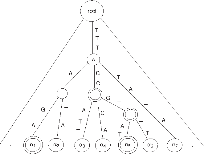end{document} is obtained as follows (see Fig. 1 for an illustration):

1. For each string α ∈ str(w) except heavypath(w), find p = 1 + |LCP(α, heavypath(w))|, that is, the position where the first mismatch occurs while matching the prefixes of α and heavypath(w).

2. Obtain a new string α′ from α by changing the character of α at position p to the character of heavypath(w) at the same position p. Specifically, α′ = α^{{(p,heavypath(w)[p])}}. Therefore, |LCP1(α, heavypath(w))| = |LCP(α′, heavypath(w))|.

3. Then \documentclass{aastex}\usepackage{amsbsy}\usepackage{amsfonts}\usepackage{amssymb}\usepackage{bm}\usepackage{mathrsfs}\usepackage{pifont}\usepackage{stmaryrd}\usepackage{textcomp}\usepackage{portland, xspace}\usepackage{amsmath, amsxtra}\pagestyle{empty}\DeclareMathSizes{10}{9}{7}{6}\begin{document} $${ \cal S}_{x^{ \prime}}$$ \end{document} is the union of str(w) and the set of (|str(w)|−1) newly created strings with respect to heavypath(w).

OPEN IN VIEWER

FIG. 1.

The heavy nodes are drawn as double circles. Here α₁ = TTTAGA, α₂ = TTTATA, α₃ = TTTCCATT, etc. str(w) = {α₁,…,α₇}, and heavypath(w) = α₅ = TTTCCGTAT. Therefore, set corresponding to w is str(w) \documentclass{aastex}\usepackage{amsbsy}\usepackage{amsfonts}\usepackage{amssymb}\usepackage{bm}\usepackage{mathrsfs}\usepackage{pifont}\usepackage{stmaryrd}\usepackage{textcomp}\usepackage{portland, xspace}\usepackage{amsmath, amsxtra}\pagestyle{empty}\DeclareMathSizes{10}{9}{7}{6}\begin{document} $$\cup \ \{ \alpha_1^{ \prime} , \alpha_2^{ \prime} , \alpha_3^{ \prime} , \alpha_4^{ \prime} , \alpha_6^{ \prime} , \alpha_7^{ \prime} \} $$ \end{document} , where \documentclass{aastex}\usepackage{amsbsy}\usepackage{amsfonts}\usepackage{amssymb}\usepackage{bm}\usepackage{mathrsfs}\usepackage{pifont}\usepackage{stmaryrd}\usepackage{textcomp}\usepackage{portland, xspace}\usepackage{amsmath, amsxtra}\pagestyle{empty}\DeclareMathSizes{10}{9}{7}{6}\begin{document} $$\alpha_1^{ \prime}$$ \end{document}  = TTTCGA, \documentclass{aastex}\usepackage{amsbsy}\usepackage{amsfonts}\usepackage{amssymb}\usepackage{bm}\usepackage{mathrsfs}\usepackage{pifont}\usepackage{stmaryrd}\usepackage{textcomp}\usepackage{portland, xspace}\usepackage{amsmath, amsxtra}\pagestyle{empty}\DeclareMathSizes{10}{9}{7}{6}\begin{document} $$\alpha_2^{ \prime}$$ \end{document}  = TTTCTA, \documentclass{aastex}\usepackage{amsbsy}\usepackage{amsfonts}\usepackage{amssymb}\usepackage{bm}\usepackage{mathrsfs}\usepackage{pifont}\usepackage{stmaryrd}\usepackage{textcomp}\usepackage{portland, xspace}\usepackage{amsmath, amsxtra}\pagestyle{empty}\DeclareMathSizes{10}{9}{7}{6}\begin{document} $$\alpha_3^{ \prime}$$ \end{document}  = TTTCCGTT, \documentclass{aastex}\usepackage{amsbsy}\usepackage{amsfonts}\usepackage{amssymb}\usepackage{bm}\usepackage{mathrsfs}\usepackage{pifont}\usepackage{stmaryrd}\usepackage{textcomp}\usepackage{portland, xspace}\usepackage{amsmath, amsxtra}\pagestyle{empty}\DeclareMathSizes{10}{9}{7}{6}\begin{document} $$\alpha_4^{ \prime}$$ \end{document}  = TTTCCGA, \documentclass{aastex}\usepackage{amsbsy}\usepackage{amsfonts}\usepackage{amssymb}\usepackage{bm}\usepackage{mathrsfs}\usepackage{pifont}\usepackage{stmaryrd}\usepackage{textcomp}\usepackage{portland, xspace}\usepackage{amsmath, amsxtra}\pagestyle{empty}\DeclareMathSizes{10}{9}{7}{6}\begin{document} $$\alpha_6^{ \prime}$$ \end{document}  = TTTCCGTAT, and \documentclass{aastex}\usepackage{amsbsy}\usepackage{amsfonts}\usepackage{amssymb}\usepackage{bm}\usepackage{mathrsfs}\usepackage{pifont}\usepackage{stmaryrd}\usepackage{textcomp}\usepackage{portland, xspace}\usepackage{amsmath, amsxtra}\pagestyle{empty}\DeclareMathSizes{10}{9}{7}{6}\begin{document} $$\alpha_7^{ \prime}$$ \end{document}  = TTTCATA.

Clearly, \documentclass{aastex}\usepackage{amsbsy}\usepackage{amsfonts}\usepackage{amssymb}\usepackage{bm}\usepackage{mathrsfs}\usepackage{pifont}\usepackage{stmaryrd}\usepackage{textcomp}\usepackage{portland, xspace}\usepackage{amsmath, amsxtra}\pagestyle{empty}\DeclareMathSizes{10}{9}{7}{6}\begin{document} $$\mid { \cal S}_{x^{ \prime}} \mid = ( 2 \mid { \sf str} ( w ) \mid - 1 ) = O ( \mid { \cal S}_x \mid )$$ \end{document} . The number of sets (associated with the children of x) in which a particular string in \documentclass{aastex}\usepackage{amsbsy}\usepackage{amsfonts}\usepackage{amssymb}\usepackage{bm}\usepackage{mathrsfs}\usepackage{pifont}\usepackage{stmaryrd}\usepackage{textcomp}\usepackage{portland, xspace}\usepackage{amsmath, amsxtra}\pagestyle{empty}\DeclareMathSizes{10}{9}{7}{6}\begin{document} $${ \cal S}_x$$ \end{document} or a modified version of it belongs to is bounded by the maximum number of light ancestors of any node in \documentclass{aastex}\usepackage{amsbsy}\usepackage{amsfonts}\usepackage{amssymb}\usepackage{bm}\usepackage{mathrsfs}\usepackage{pifont}\usepackage{stmaryrd}\usepackage{textcomp}\usepackage{portland, xspace}\usepackage{amsmath, amsxtra}\pagestyle{empty}\DeclareMathSizes{10}{9}{7}{6}\begin{document} $${ \cal T}$$ \end{document} , which is \documentclass{aastex}\usepackage{amsbsy}\usepackage{amsfonts}\usepackage{amssymb}\usepackage{bm}\usepackage{mathrsfs}\usepackage{pifont}\usepackage{stmaryrd}\usepackage{textcomp}\usepackage{portland, xspace}\usepackage{amsmath, amsxtra}\pagestyle{empty}\DeclareMathSizes{10}{9}{7}{6}\begin{document} $$\log \mid { \cal S}_x \mid$$ \end{document} . This gives an upper bound \documentclass{aastex}\usepackage{amsbsy}\usepackage{amsfonts}\usepackage{amssymb}\usepackage{bm}\usepackage{mathrsfs}\usepackage{pifont}\usepackage{stmaryrd}\usepackage{textcomp}\usepackage{portland, xspace}\usepackage{amsmath, amsxtra}\pagestyle{empty}\DeclareMathSizes{10}{9}{7}{6}\begin{document} $$2 \mid { \cal S}_x \mid \log \mid { \cal S}_x \mid$$ \end{document} on the sum of sizes of the sets associated with the children of x. Finally, let \documentclass{aastex}\usepackage{amsbsy}\usepackage{amsfonts}\usepackage{amssymb}\usepackage{bm}\usepackage{mathrsfs}\usepackage{pifont}\usepackage{stmaryrd}\usepackage{textcomp}\usepackage{portland, xspace}\usepackage{amsmath, amsxtra}\pagestyle{empty}\DeclareMathSizes{10}{9}{7}{6}\begin{document} $${ \sf X}_i^{ \Delta}$$ \end{document} and \documentclass{aastex}\usepackage{amsbsy}\usepackage{amsfonts}\usepackage{amssymb}\usepackage{bm}\usepackage{mathrsfs}\usepackage{pifont}\usepackage{stmaryrd}\usepackage{textcomp}\usepackage{portland, xspace}\usepackage{amsmath, amsxtra}\pagestyle{empty}\DeclareMathSizes{10}{9}{7}{6}\begin{document} $${ \sf Y}_j^{ \Delta^{ \prime}}$$ \end{document} be two modified suffixes in \documentclass{aastex}\usepackage{amsbsy}\usepackage{amsfonts}\usepackage{amssymb}\usepackage{bm}\usepackage{mathrsfs}\usepackage{pifont}\usepackage{stmaryrd}\usepackage{textcomp}\usepackage{portland, xspace}\usepackage{amsmath, amsxtra}\pagestyle{empty}\DeclareMathSizes{10}{9}{7}{6}\begin{document} $${ \cal S}_x$$ \end{document} that form an (i, j)_h−1-maxpair, and let u (resp., w) be the lowest common ancestor (resp., light ancestor) of the leaves corresponding to them in \documentclass{aastex}\usepackage{amsbsy}\usepackage{amsfonts}\usepackage{amssymb}\usepackage{bm}\usepackage{mathrsfs}\usepackage{pifont}\usepackage{stmaryrd}\usepackage{textcomp}\usepackage{portland, xspace}\usepackage{amsmath, amsxtra}\pagestyle{empty}\DeclareMathSizes{10}{9}{7}{6}\begin{document} $${ \cal T}$$ \end{document} . Then, our method creates a set corresponding to w, such that it contains two modified suffixes \documentclass{aastex}\usepackage{amsbsy}\usepackage{amsfonts}\usepackage{amssymb}\usepackage{bm}\usepackage{mathrsfs}\usepackage{pifont}\usepackage{stmaryrd}\usepackage{textcomp}\usepackage{portland, xspace}\usepackage{amsmath, amsxtra}\pagestyle{empty}\DeclareMathSizes{10}{9}{7}{6}\begin{document} $${ \sf X}_i^{ \Delta^{ \prime \prime}}$$ \end{document} and \documentclass{aastex}\usepackage{amsbsy}\usepackage{amsfonts}\usepackage{amssymb}\usepackage{bm}\usepackage{mathrsfs}\usepackage{pifont}\usepackage{stmaryrd}\usepackage{textcomp}\usepackage{portland, xspace}\usepackage{amsmath, amsxtra}\pagestyle{empty}\DeclareMathSizes{10}{9}{7}{6}\begin{document} $${ \sf Y}_j^{ \Delta^{ \prime \prime \prime}}$$ \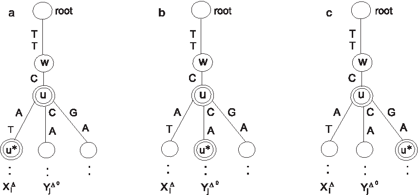end{document} that form an (i, j) _h -maxpair. Specifically, Δ″ and Δ′″ are as follows (see Fig. 2 for an illustration):

(a) If the heavy child of u, say u*, is an ancestor of the leaf corresponding to \documentclass{aastex}\usepackage{amsbsy}\usepackage{amsfonts}\usepackage{amssymb}\usepackage{bm}\usepackage{mathrsfs}\usepackage{pifont}\usepackage{stmaryrd}\usepackage{textcomp}\usepackage{portland, xspace}\usepackage{amsmath, amsxtra}\pagestyle{empty}\DeclareMathSizes{10}{9}{7}{6}\begin{document} $${ \sf X}_i^{ \Delta}$$ \end{document} , then Δ′′ = Δ and Δ′′′ = Δ′∪{(p, X _i [p])}, where p = 1 plus string depth of u. ^†

(b) If u* is an ancestor of the leaf corresponding to \documentclass{aastex}\usepackage{amsbsy}\usepackage{amsfonts}\usepackage{amssymb}\usepackage{bm}\usepackage{mathrsfs}\usepackage{pifont}\usepackage{stmaryrd}\usepackage{textcomp}\usepackage{portland, xspace}\usepackage{amsmath, amsxtra}\pagestyle{empty}\DeclareMathSizes{10}{9}{7}{6}\begin{document} $${ \sf Y}_j^{ \Delta^{ \prime}}$$ \end{document} , then Δ′′ = Δ ∪{(p, Y _j [p])} and Δ′′′ = Δ′.

(c) If neither of the above is true, then we have Δ″ = Δ ∪{(p, heavypath(w)[p])} and Δ′′′ = Δ′∪{(p, heavypath(w)[p])}.

OPEN IN VIEWER

FIG. 2.

Heavy nodes are drawn as double circles. In this example, u is heavy, the string depth of u is 3, and p = 4. Then, Δ′′′ = Δ′∪{[4, A]} in case(a), Δ′′ = Δ ∪{[4, C]} in case(b), and Δ′′ = Δ ∪{[4, G]}, Δ′′′ = Δ′∪{[4, G]} in case(c).

4.1.1. Time and space complexity

The above recursive step can be executed as follows: First, construct \documentclass{aastex}\usepackage{amsbsy}\usepackage{amsfonts}\usepackage{amssymb}\usepackage{bm}\usepackage{mathrsfs}\usepackage{pifont}\usepackage{stmaryrd}\usepackage{textcomp}\usepackage{portland, xspace}\usepackage{amsmath, amsxtra}\pagestyle{empty}\DeclareMathSizes{10}{9}{7}{6}\begin{document} $${ \cal T}$$ \end{document} using the following steps.

1. Lexicographically sort all modified suffixes in \documentclass{aastex}\usepackage{amsbsy}\usepackage{amsfonts}\usepackage{amssymb}\usepackage{bm}\usepackage{mathrsfs}\usepackage{pifont}\usepackage{stmaryrd}\usepackage{textcomp}\usepackage{portland, xspace}\usepackage{amsmath, amsxtra}\pagestyle{empty}\DeclareMathSizes{10}{9}{7}{6}\begin{document} $$O ( \mid { \cal S}_x \mid )$$ \end{document} . We shall use the result in Lemma 2 and perform this step in \documentclass{aastex}\usepackage{amsbsy}\usepackage{amsfonts}\usepackage{amssymb}\usepackage{bm}\usepackage{mathrsfs}\usepackage{pifont}\usepackage{stmaryrd}\usepackage{textcomp}\usepackage{portland, xspace}\usepackage{amsmath, amsxtra}\pagestyle{empty}\DeclareMathSizes{10}{9}{7}{6}\begin{document} $$O ( \mid { \cal S}_x \mid \log \mid { \cal S}_x \mid )$$ \end{document} time.

2. Compute |LCP(·,·)| between all consecutive pairs of modified suffixes in \documentclass{aastex}\usepackage{amsbsy}\usepackage{amsfonts}\usepackage{amssymb}\usepackage{bm}\usepackage{mathrsfs}\usepackage{pifont}\usepackage{stmaryrd}\usepackage{textcomp}\usepackage{portland, xspace}\usepackage{amsmath, amsxtra}\pagestyle{empty}\DeclareMathSizes{10}{9}{7}{6}\begin{document} $${ \cal S}_x$$ \end{document} . Using GST, we can execute this step in \documentclass{aastex}\usepackage{amsbsy}\usepackage{amsfonts}\usepackage{amssymb}\usepackage{bm}\usepackage{mathrsfs}\usepackage{pifont}\usepackage{stmaryrd}\usepackage{textcomp}\usepackage{portland, xspace}\usepackage{amsmath, amsxtra}\pagestyle{empty}\DeclareMathSizes{10}{9}{7}{6}\begin{document} $$O ( \mid { \cal S}_x \mid )$$ \end{document} time using Lemma 1.

3. Finally, to construct \documentclass{aastex}\usepackage{amsbsy}\usepackage{amsfonts}\usepackage{amssymb}\usepackage{bm}\usepackage{mathrsfs}\usepackage{pifont}\usepackage{stmaryrd}\usepackage{textcomp}\usepackage{portland, xspace}\usepackage{amsmath, amsxtra}\pagestyle{empty}\DeclareMathSizes{10}{9}{7}{6}\begin{document} $${ \cal T}$$ \end{document} using the results from Step (1) and Step (2), we borrow well-known techniques from the suffix tree construction literature [Farach-Colton et al., 2000): a patricia tree over a set of strings can be constructed in time linear in the number of strings, given the lexicographical ordering of all strings and length of the longest common prefix of all pairs of consecutive leaves of the tree. Therefore, time complexity is \documentclass{aastex}\usepackage{amsbsy}\usepackage{amsfonts}\usepackage{amssymb}\usepackage{bm}\usepackage{mathrsfs}\usepackage{pifont}\usepackage{stmaryrd}\usepackage{textcomp}\usepackage{portland, xspace}\usepackage{amsmath, amsxtra}\pagestyle{empty}\DeclareMathSizes{10}{9}{7}{6}\begin{document} $$O ( \mid { \cal S}_x \mid )$$ \end{document} .

Once \documentclass{aastex}\usepackage{amsbsy}\usepackage{amsfonts}\usepackage{amssymb}\usepackage{bm}\usepackage{mathrsfs}\usepackage{pifont}\usepackage{stmaryrd}\usepackage{textcomp}\usepackage{portland, xspace}\usepackage{amsmath, amsxtra}\pagestyle{empty}\DeclareMathSizes{10}{9}{7}{6}\begin{document} $${ \cal T}$$ \end{document} is constructed, all light internal nodes can be identified by a linear time tree traversal. Each light node w is then visited and the set corresponding to it is constructed in O(|str(w)|) time. The total time is proportional to the \documentclass{aastex}\usepackage{amsbsy}\usepackage{amsfonts}\usepackage{amssymb}\usepackage{bm}\usepackage{mathrsfs}\usepackage{pifont}\usepackage{stmaryrd}\usepackage{textcomp}\usepackage{portland, xspace}\usepackage{amsmath, amsxtra}\pagestyle{empty}\DeclareMathSizes{10}{9}{7}{6}\begin{document} $${ \cal S}_x$$ \end{document} plus the sum of sizes of all newly created sets, that is, \documentclass{aastex}\usepackage{amsbsy}\usepackage{amsfonts}\usepackage{amssymb}\usepackage{bm}\usepackage{mathrsfs}\usepackage{pifont}\usepackage{stmaryrd}\usepackage{textcomp}\usepackage{portland, xspace}\usepackage{amsmath, amsxtra}\pagestyle{empty}\DeclareMathSizes{10}{9}{7}{6}\begin{document} $$O ( \mid { \cal S}_x \mid \log \mid { \cal S}_x \mid )$$ \end{document} . Therefore, time for constructing TREE is \documentclass{aastex}\usepackage{amsbsy}\usepackage{amsfonts}\usepackage{amssymb}\usepackage{bm}\usepackage{mathrsfs}\usepackage{pifont}\usepackage{stmaryrd}\usepackage{textcomp}\usepackage{portland, xspace}\usepackage{amsmath, amsxtra}\pagestyle{empty}\DeclareMathSizes{10}{9}{7}{6}\begin{document} $$\sum \nolimits_{x \in { \rm NODES}} \mid { \cal S}_x \mid = O ( n \log^k n )$$ \end{document} .

Since we are not interested in storing the members of the partition, but just create, process, and discard them, the nodes in TREE can be created in the order of depth first search, so that at any point in time, we need to maintain nodes (and associated sets) in only one root to leaf path. Therefore, \documentclass{aastex}\usepackage{amsbsy}\usepackage{amsfonts}\usepackage{amssymb}\usepackage{bm}\usepackage{mathrsfs}\usepackage{pifont}\usepackage{stmaryrd}\usepackage{textcomp}\usepackage{portland, xspace}\usepackage{amsmath, amsxtra}\pagestyle{empty}\DeclareMathSizes{10}{9}{7}{6}\begin{document} $$O ( k \times \max \nolimits_{x \in { \rm NODES}} \mid { \cal S}_x \mid ) = O ( n )$$ \end{document} working space is sufficient. This completes phase 1 of our algorithm.

5. Phase 2: Processing the Partition

In this section, we describe how to process each member \documentclass{aastex}\usepackage{amsbsy}\usepackage{amsfonts}\usepackage{amssymb}\usepackage{bm}\usepackage{mathrsfs}\usepackage{pifont}\usepackage{stmaryrd}\usepackage{textcomp}\usepackage{portland, xspace}\usepackage{amsmath, amsxtra}\pagestyle{empty}\DeclareMathSizes{10}{9}{7}{6}\begin{document} $${ \cal P}_f$$ \end{document} of the partition independently. Let \documentclass{aastex}\usepackage{amsbsy}\usepackage{amsfonts}\usepackage{amssymb}\usepackage{bm}\usepackage{mathrsfs}\usepackage{pifont}\usepackage{stmaryrd}\usepackage{textcomp}\usepackage{portland, xspace}\usepackage{amsmath, amsxtra}\pagestyle{empty}\DeclareMathSizes{10}{9}{7}{6}\begin{document} $$\Lambda [ 1 , \mid { \sf X} \mid ]$$ \end{document} be an integer array of length |X| with all its entries initialized to 0. While processing the members, we update this array in such a way that after processing all members in the partition, we obtain \documentclass{aastex}\usepackage{amsbsy}\usepackage{amsfonts}\usepackage{amssymb}\usepackage{bm}\usepackage{mathrsfs}\usepackage{pifont}\usepackage{stmaryrd}\usepackage{textcomp}\usepackage{portland, xspace}\usepackage{amsmath, amsxtra}\pagestyle{empty}\DeclareMathSizes{10}{9}{7}{6}\begin{document} $$\lambda_k ( { \sf X}_i , { \sf Y} ) = \Lambda [ i ]$$ \end{document} . To process a particular \documentclass{aastex}\usepackage{amsbsy}\usepackage{amsfonts}\usepackage{amssymb}\usepackage{bm}\usepackage{mathrsfs}\usepackage{pifont}\usepackage{stmaryrd}\usepackage{textcomp}\usepackage{portland, xspace}\usepackage{amsmath, amsxtra}\pagestyle{empty}\DeclareMathSizes{10}{9}{7}{6}\begin{document} $${ \cal P}_f$$ \end{document} , we follow the steps below:

1. Create all nonempty subsets (called pi-sets) derived from \documentclass{aastex}\usepackage{amsbsy}\usepackage{amsfonts}\usepackage{amssymb}\usepackage{bm}\usepackage{mathrsfs}\usepackage{pifont}\usepackage{stmaryrd}\usepackage{textcomp}\usepackage{portland, xspace}\usepackage{amsmath, amsxtra}\pagestyle{empty}\DeclareMathSizes{10}{9}{7}{6}\begin{document} $${ \cal P}_f$$ \end{document} as defined below: \documentclass{aastex}\usepackage{amsbsy}\usepackage{amsfonts}\usepackage{amssymb}\usepackage{bm}\usepackage{mathrsfs}\usepackage{pifont}\usepackage{stmaryrd}\usepackage{textcomp}\usepackage{portland, xspace}\usepackage{amsmath, amsxtra}\pagestyle{empty}\DeclareMathSizes{10}{9}{7}{6}\begin{document} \begin{align*}\Pi_{ ( \delta , x , y ) } = \{ { \sf X}_i^{ \Delta} \in { \cal P}_f \mid \delta \subseteq \Delta \ { \rm and} \ \mid \Delta \mid = x \} \cup \{ { \sf Y}_j^{ \Delta^{ \prime}} \in { \cal P}_f \mid \delta \subseteq \Delta^{ \prime} \ { \rm and} \ \mid \Delta^{ \prime} \mid = y \} \end{align*} \end{document}

Here δ is a set of (position, character) pairs and x, y are integers in [0, k].

Correctness: To prove that λ_k(X _i , Y) = Λ[i] after processing all members, consider a fixed i, where λ_k(X _i , Y) = |LCP _k (X _i , Y_j*)|. While processing the member that contains an (i, j*) _k -maxpair (say \documentclass{aastex}\usepackage{amsbsy}\usepackage{amsfonts}\usepackage{amssymb}\usepackage{bm}\usepackage{mathrsfs}\usepackage{pifont}\usepackage{stmaryrd}\usepackage{textcomp}\usepackage{portland, xspace}\usepackage{amsmath, amsxtra}\pagestyle{empty}\DeclareMathSizes{10}{9}{7}{6}\begin{document} $${ \sf X}_i^{ \Delta_1}$$ \end{document} and \documentclass{aastex}\usepackage{amsbsy}\usepackage{amsfonts}\usepackage{amssymb}\usepackage{bm}\usepackage{mathrsfs}\usepackage{pifont}\usepackage{stmaryrd}\usepackage{textcomp}\usepackage{portland, xspace}\usepackage{amsmath, amsxtra}\pagestyle{empty}\DeclareMathSizes{10}{9}{7}{6}\begin{document} $${ \sf Y}_{j^*}^{ \Delta_2}$$ \end{document} ), a pi-set \documentclass{aastex}\usepackage{amsbsy}\usepackage{amsfonts}\usepackage{amssymb}\usepackage{bm}\usepackage{mathrsfs}\usepackage{pifont}\usepackage{stmaryrd}\usepackage{textcomp}\usepackage{portland, xspace}\usepackage{amsmath, amsxtra}\pagestyle{empty}\DeclareMathSizes{10}{9}{7}{6}\begin{document} $$\Pi_{ ( \Delta_1 \cap \Delta_2 , \mid \Delta_1 \mid , \mid \Delta_2 \mid ) }$$ \end{document} will be created, and while processing this particular pi-set, Λ[i] will be updated to \documentclass{aastex}\usepackage{amsbsy}\usepackage{amsfonts}\usepackage{amssymb}\usepackage{bm}\usepackage{mathrsfs}\usepackage{pifont}\usepackage{stmaryrd}\usepackage{textcomp}\usepackage{portland, xspace}\usepackage{amsmath, amsxtra}\pagestyle{empty}\DeclareMathSizes{10}{9}{7}{6}\begin{document} $$\mid { \sf LCP}_k ( { \sf X}_i , { \sf Y}_{j^*} ) \mid$$ \end{document} .

Analysis: Step 1 can be implemented as follows.

1. For each \documentclass{aastex}\usepackage{amsbsy}\usepackage{amsfonts}\usepackage{amssymb}\usepackage{bm}\usepackage{mathrsfs}\usepackage{pifont}\usepackage{stmaryrd}\usepackage{textcomp}\usepackage{portland, xspace}\usepackage{amsmath, amsxtra}\pagestyle{empty}\DeclareMathSizes{10}{9}{7}{6}\begin{document} $${ \sf X}_i^{ \Delta} \in { \cal P}_f$$ \end{document} , generate a (set, string) pair of the form ( \documentclass{aastex}\usepackage{amsbsy}\usepackage{amsfonts}\usepackage{amssymb}\usepackage{bm}\usepackage{mathrsfs}\usepackage{pifont}\usepackage{stmaryrd}\usepackage{textcomp}\usepackage{portland, xspace}\usepackage{amsmath, amsxtra}\pagestyle{empty}\DeclareMathSizes{10}{9}{7}{6}\begin{document} $$( \delta , { \sf X}_i^{ \Delta} )$$ \end{document} ) for each δ ⊆ Δ. Similarly, for each \documentclass{aastex}\usepackage{amsbsy}\usepackage{amsfonts}\usepackage{amssymb}\usepackage{bm}\usepackage{mathrsfs}\usepackage{pifont}\usepackage{stmaryrd}\usepackage{textcomp}\usepackage{portland, xspace}\usepackage{amsmath, amsxtra}\pagestyle{empty}\DeclareMathSizes{10}{9}{7}{6}\begin{document} $${ \sf Y}_j^{ \Delta^{ \prime}} \in { \cal P}_f$$ \end{document} , generate pair ( \documentclass{aastex}\usepackage{amsbsy}\usepackage{amsfonts}\usepackage{amssymb}\usepackage{bm}\usepackage{mathrsfs}\usepackage{pifont}\usepackage{stmaryrd}\usepackage{textcomp}\usepackage{portland, xspace}\usepackage{amsmath, amsxtra}\pagestyle{empty}\DeclareMathSizes{10}{9}{7}{6}\begin{document} $$( \delta , { \sf Y}_j^{ \Delta^{ \prime}} )$$ \end{document} ) for each δ ⊆ Δ′. Therefore, the number of pairs is \documentclass{aastex}\usepackage{amsbsy}\usepackage{amsfonts}\usepackage{amssymb}\usepackage{bm}\usepackage{mathrsfs}\usepackage{pifont}\usepackage{stmaryrd}\usepackage{textcomp}\usepackage{portland, xspace}\usepackage{amsmath, amsxtra}\pagestyle{empty}\DeclareMathSizes{10}{9}{7}{6}\begin{document} $$\leq 2^k \mid { \cal P}_f \mid$$ \end{document} .

Essentially, step 1 involves sorting and scanning several sets of integers of total cardinality \documentclass{aastex}\usepackage{amsbsy}\usepackage{amsfonts}\usepackage{amssymb}\usepackage{bm}\usepackage{mathrsfs}\usepackage{pifont}\usepackage{stmaryrd}\usepackage{textcomp}\usepackage{portland, xspace}\usepackage{amsmath, amsxtra}\pagestyle{empty}\DeclareMathSizes{10}{9}{7}{6}\begin{document} $$O ( \mid { \cal P}_f \mid )$$ \end{document} . The key operations involved in step 2 are also the same. Therefore, a particular \documentclass{aastex}\usepackage{amsbsy}\usepackage{amsfonts}\usepackage{amssymb}\usepackage{bm}\usepackage{mathrsfs}\usepackage{pifont}\usepackage{stmaryrd}\usepackage{textcomp}\usepackage{portland, xspace}\usepackage{amsmath, amsxtra}\pagestyle{empty}\DeclareMathSizes{10}{9}{7}{6}\begin{document} $${ \cal P}_f$$ \end{document} can be processed in \documentclass{aastex}\usepackage{amsbsy}\usepackage{amsfonts}\usepackage{amssymb}\usepackage{bm}\usepackage{mathrsfs}\usepackage{pifont}\usepackage{stmaryrd}\usepackage{textcomp}\usepackage{portland, xspace}\usepackage{amsmath, amsxtra}\pagestyle{empty}\DeclareMathSizes{10}{9}{7}{6}\begin{document} $$O ( \mid { \cal P}_f \mid \log \mid { \cal P}_f \mid )$$ \end{document} time using \documentclass{aastex}\usepackage{amsbsy}\usepackage{amsfonts}\usepackage{amssymb}\usepackage{bm}\usepackage{mathrsfs}\usepackage{pifont}\usepackage{stmaryrd}\usepackage{textcomp}\usepackage{portland, xspace}\usepackage{amsmath, amsxtra}\pagestyle{empty}\DeclareMathSizes{10}{9}{7}{6}\begin{document} $$O ( n + \mid { \cal P}_f \mid )$$ \end{document} working space. Therefore, we can implement phase 2 in \documentclass{aastex}\usepackage{amsbsy}\usepackage{amsfonts}\usepackage{amssymb}\usepackage{bm}\usepackage{mathrsfs}\usepackage{pifont}\usepackage{stmaryrd}\usepackage{textcomp}\usepackage{portland, xspace}\usepackage{amsmath, amsxtra}\pagestyle{empty}\DeclareMathSizes{10}{9}{7}{6}\begin{document} $$O ( n + \max \nolimits_f \mid { \cal P}_f \mid ) = O ( n )$$ \end{document} space and \documentclass{aastex}\usepackage{amsbsy}\usepackage{amsfonts}\usepackage{amssymb}\usepackage{bm}\usepackage{mathrsfs}\usepackage{pifont}\usepackage{stmaryrd}\usepackage{textcomp}\usepackage{portland, xspace}\usepackage{amsmath, amsxtra}\pagestyle{empty}\DeclareMathSizes{10}{9}{7}{6}\begin{document} $$O ( n \log^k n + \sum \nolimits_f \mid { \cal P}_f \mid \log \mid { \cal P}_f \mid ) = O ( n \log^{k + 1}n )$$ \end{document} time.

6. Conclusions

We present an efficient algorithm for the k-mismatch average common substring problem that runs in O(n log^kn) time and O(n) space. This constitutes a significant improvement over the O(n²) worst case run-time of the prior state of the art. In the absence of the proposed space-saving technique, our algorithm would have taken O(n log ^k n) space, which would be impractical for even small values of k. Our algorithm achieves linear working space by decomposing the set of modified suffixes so that they can be processed and discarded independently, while preserving the ability to bring pairs of modified suffixes together. Note that the biological applications of ACS _k are well documented in Leimeister and Morgenstern (2014). The vastly improved efficiency in computing ACS _k by our algorithm should naturally impact these applications positively.