Rapidly Registering Identity-by-Descent Across Ancestral Recombination Graphs

Abstract

The genomes of remotely related individuals occasionally contain long segments that are identical by descent (IBD). Sharing of IBD segments has many applications in population and medical genetics, and it is thus desirable to study their properties in simulations. However, no current method provides a direct, efficient means to extract IBD segments from simulated genealogies. Here, we introduce computationally efficient approaches to extract ground-truth IBD segments from a sequence of genealogies, or equivalently, an ancestral recombination graph. Specifically, we use a two-step scheme, where we first identify putative shared segments by comparing the common ancestors of all pairs of individuals at some distance apart. This reduces the search space considerably, and we then proceed by determining the true IBD status of the candidate segments. Under some assumptions and when allowing a limited resolution of segment lengths, our run-time complexity is reduced from O(n³ log n) for the naïve algorithm to O(n log n), where n is the number of individuals in the sample.

1. Introduction

Segments in the genomes of two individuals that are inherited from a single most recent common ancestor are said to be identical-by-descent (IBD). Such segments have many applications in medical and population genetics (Gusev et al., 2011, 2012; Albrechtsen et al., 2010). For example, IBD segments are useful for identifying relatives (Huff et al., 2011; Henn et al., 2012b), and, using various inference methods, the observed number and lengths of IBD segments can be used to reconstruct the demographic history of populations (Palamara et al., 2012; Carmi et al., 2013; Ralph and Coop, 2013; Mathieson and McVean, 2014; Palamara and Pe'er, 2013; Carmi et al., 2014b).

Multiple inference paradigms, such as approximate Bayesian computation (Beaumont et al., 2002) or importance sampling (Fearnhead and Donnelly, 2001), are based on sampling from a probability space defined by the hypothesized model for the data. In the context of demographic inference, these methods require simulating IBD segments often based on complicated models for histories of populations. Naively, this would be carried out by simulating genetic data using genome simulators (e.g., Excoffier and Foll, 2011; Excoffier et al., 2013; Schaffner et al., 2005; Liang et al., 2007, followed by computational recovery of IBD segments (e.g., Gusev et al., 2009; Browning and Browning 2011). However, this process is both computationally intensive, therefore limiting sample sizes, as well as error prone, contrasting with its role of producing ground-truth simulated data.

In addition to the computational burden, inference of IBD segments from simulated sequences is also redundant, in the sense that information about IBD segments is intrinsic to the simulated genealogies, without the need to explicitly generate the entire sequences. Specifically, genetic data simulated according to the coalescent with recombination is represented as an ancestral recombination graph (ARG), a combinatorial structure that has the genealogies of the entire sample at all positions along the chromosome (see Hudson, 1990; Griffiths and Marjoram, 1996, 1997; and below for definitions). Equivalently, the ARG can be represented as a sequence of genealogical (or “coalescent”) trees, where each new tree is formed due to a recombination event in the history of the sample (Wiuf and Hein, 1999). Our goal in this work is to efficiently scan such a series of trees for IBD segments, that is, find all contiguous segments where pairs of individuals share the same common ancestor. Previous studies have either employed a naïve algorithm (see below; Browning and Browning, 2013; Tataru et al., 2014; Chiang et al., 2014) or avoided coalescent simulations by using permutations of real genotypes (Gusev et al., 2009; Browning and Browning, 2011; Su et al., 2012).

The article is organized as follows. In section 2, we introduce notation and models. In section 3, we describe a series of computational approaches for extracting ground-truth IBD segments from ARGs. In section 3.1, a naïve algorithm is presented. In section 3.2, we analyze the complexity of the algorithm when segment lengths are discretized. In section 3.3, we describe a two-step approach for segment discovery, which is based on decoupling the problem into first identifying a small set of “candidate” pairs and segments, some of which are false but which include all true segments. Then, taking advantage of the constant time LCA query algorithm, we rapidly eliminate all false positives. In section 3.4, we present a fast algorithm to compare the common ancestors of all pairs of leaves between two trees, which, when segment lengths are discretized and combined with the two-step approach, achieves the best asymptotic run-time complexity. In section 4, we present performance benchmarks demonstrating utility for practical applications. In section 5, we demonstrate the application of our tool in demographic inference, and in section 6, we discuss limitations and future plans. The implementation of our algorithms is freely available (Yang, 2014).

2. Preliminaries

We are given a sample of n individuals, each of which is represented by a single continuous chromosome of length L Morgans (M). The ancestry of the sample is denoted by a series of trees, {T_i}, i = 0,…,n_T, each defined along a genomic interval, [x_i, x_i₊₁) (where x₀ = 0, x_n_{_T} = x_n_{_T}₊₁ = L and the last tree is degenerate). The tree at each genomic position corresponds to the genealogy of the individuals at that position (Fig. 1). Genealogies are formed according to the coalescent (Wakeley, 2005): Each pair of lineages merges, going backward in time, at rate 1/N, where N is the effective population size. Intervals are broken, and hence, new trees are formed, due to recombination in one of the lineages in the genealogy. Specifically, the effect of recombination is to create a breakpoint in the tree, leading to rewiring of the edges of the tree (Hudson, 1983; Wiuf and Hein, 1999). While rewiring can happen only in a limited number of ways, we do not make any assumption on the nature of the differences between successive trees. Internal nodes in the tree are formed by lineages merging into their common ancestors (going backward in time) and are labeled by the time in the past when those ancestors existed. Time is assumed to be continuous, and therefore, two internal nodes in different trees but with the same label correspond to the same ancestral individual. The collection of all trees, labels of internal nodes, and intervals is called an ancestral recombination graph (ARG) and is the input to our method.

FIG. 1.

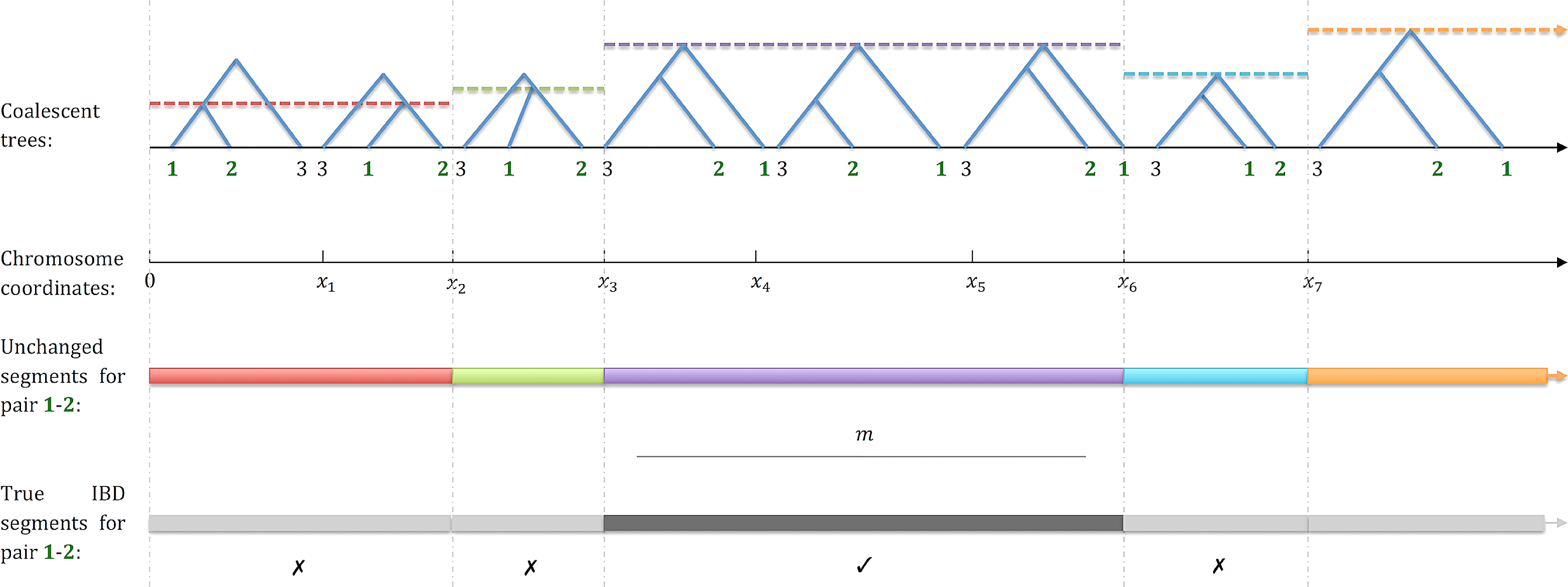
Extracting IBD segments from a sequence of coalescent trees. A series of trees for a sample of n = 3 is shown. The collection of all trees and their intervals forms an ancestral recombination graph (ARG). The time to the most recent common ancestor (tMRCA) of individuals 1 and 2 is indicated as a horizontal line for each tree. Below the trees, bars of different colors indicate the boundaries of the shared segments for this ARG and individuals 1 and 2, that is, maximal contiguous segments where the MRCA of 1 and 2 does not change. Imposing a minimal segment length m, only one segment exceeds the length cutoff (black). Other segments (gray) will not be reported.

Define a pair of individuals as IBD along a genomic interval if the interval is longer than a threshold m and the time to the most recent common ancestor (MRCA; equivalently, the lowest common ancestor [LCA]) of the individuals is the same along all the trees contained in the interval. Our desired output is the set of maximal IBD segments between all pairs of individuals, in the sense that no reported segment can be extended in either direction and remain IBD (Fig. 1). Typical values of m and L are 1 centiMorgans (cM; roughly a million base pairs) and 100cM (1M), respectively, and we treat them as constants throughout the paper. The mean number of trees is known to satisfy n_T = O(NL log n) (Griffiths and Marjoram, 1997). Running times are thus reported as functions of n and N, and occasionally, to project the result into a single dimension, we assume that N = O(n). This is realistic for human populations, where the effective population size is 10,000–20,000 (Conrad et al., 2006; Henn et al., 2012a), and current sample sizes are in the thousands (e.g., Zhang et al., 2015; Guha et al. 2012; The Wellcome Trust Case Control Consortium, 2007).

3. Methods

3.1. The naïve algorithm

The naïve algorithm works by keeping track of the time to the MRCA (tMRCA) between all pairs of chromosomes (i.e., leaves in the tree), and determining, for each tree, which tMRCAs have changed compared to the previous tree. To extract the tMRCAs of all pairs in a given tree, we used an in-order traversal algorithm (Yang, 2014). Whenever we detect a change of the tMRCA for a given pair of leaves, we report the segment as IBD if the previous tMRCA had persisted over length > m (Algorithm 1). Each comparison between trees involves all pairs of leaves and thus runs in time O (n²). As there are O (NL log n) trees, the total time complexity for the naïve algorithm is O (n²NL log n), or O (n³ log n) when treating L as a constant and assuming N = O(n).

Algorithm 1:

A naïve algorithm for reporting IBD

Naïve({T_i},{x_i})

1 for each (u, v)

2 PrevLCA[u, v] = 0, LastChanged[u, v] = 0

3 for i = 0,…,n_T

4 for each (u, v)

5 CurrLCA[u, v] = LCA of u and v in T_i

6 if CurrLCA[u, v]≠PrevLCA[u, v]

7 if x_i–LastChanged[u, v] > m

8 report((u, v), [LastChanged[u, v], x_i])

9 LastChanged[u, v] = x_i

10 PrevLCA[u, v] = CurrLCA[u, v]

3.2. Discretization of the genome

When the number of trees per unit genetic distance is large (e.g., whenever N or n are large), examining all trees has limited merit. We thus follow Browning and Browning (2013) and consider only trees at fixed tickmarks along the genome, every d = εm cM. This allows even the shortest segment length to be estimated with a relative error up to 1 ± ε, while reducing the running time to \documentclass{aastex}\usepackage{amsbsy}\usepackage{amsfonts}\usepackage{amssymb}\usepackage{bm}\usepackage{mathrsfs}\usepackage{pifont}\usepackage{stmaryrd}\usepackage{textcomp}\usepackage{portland, xspace}\usepackage{amsmath, amsxtra}\pagestyle{empty}\DeclareMathSizes{10}{9}{7}{6}\begin{document} $$O \left( \frac { L } { m \epsilon } n^2 \right) = O \left( n^2 \right)$$ \end{document} , an improvement of fold-change O (Nd log n). Discretization may introduce false negatives, such as segments of length in [m, m(1 + ε)) that appears as m(1 − ε), as well as false positives, due to individuals with an identical common ancestor at successive tickmarks but with a different ancestor between the tickmarks (see Supplementary Fig. S1 available online at www.liebertonline.com/cmb for details). However, empirical results, using ε = 0.01, demonstrate that the error is minuscule (Fig. 2). Note also that for the popular Markovian approximations of the pairwise coalescent with recombination (McVean and Cardin, 2005; Li and Durbin, 2011; Marjoram and Wall, 2006), discretization would not lead to false positives.

FIG. 2.

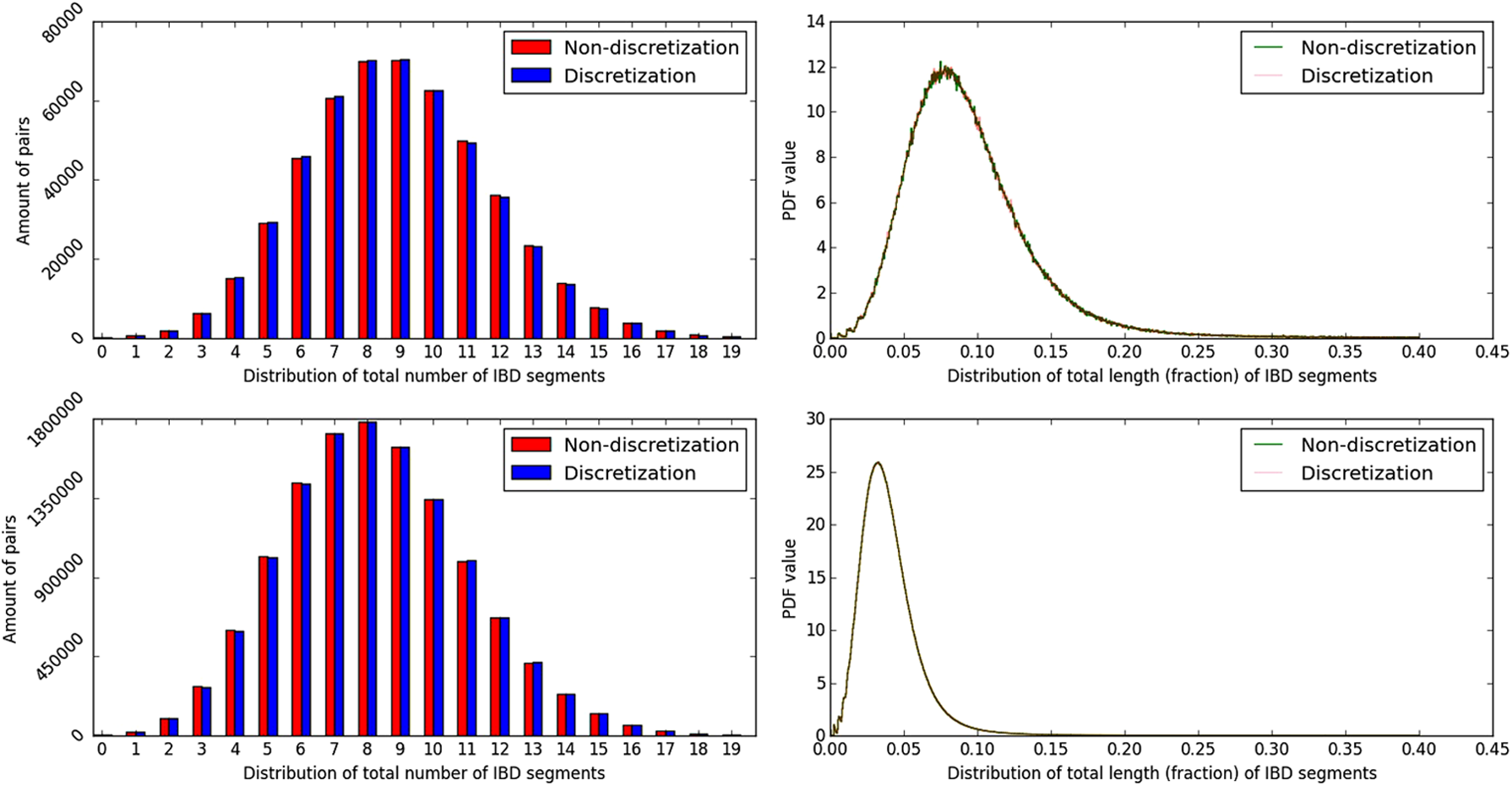
The effect of segment length discretization on the accuracy of genome-wide IBD statistics. (Left) The distribution of the total number of IBD segments shared between each pair of individuals. (Right) the density of the total fraction of the chromosome found in IBD segments. (Top) n = 1000, m = 0.00534; (bottom) n = 5000, m = 0.00245. In all panels, N = 2n, L = 1, and ε = 0.01.

3.3. A two-step approach

For typical values of m and N and in a typical genomic locus, most pairs of individuals do not maintain the same MRCA over lengths longer than m. Therefore, an appealing approach would be to rapidly eliminate, at each genomic position, all pairs of individuals that do not share an IBD segment, and then consider for validating only the remaining pairs. Specifically, when we compare the MRCAs of pairs of individuals at genomic tickmarks spaced s = m/2 apart, we observe that true IBD segments must span at least two consecutive tickmarks (Fig. 3; note that no discretization of segment lengths is assumed). For each pair of individuals that satisfies this condition, we first verify that the MRCA is unchanged in all trees between the tickmarks, and then extend the segment in both directions and determine whether the final segment length is longer than m. For the validation step, we use Bender's LCA algorithm (Bender and Farach-Colton, 2000; Berkman et al., 1989), which requires linear time to preprocess each tree, but then just a constant time for each LCA (i.e., tMRCA) query (Algorithm 2).

FIG. 3.

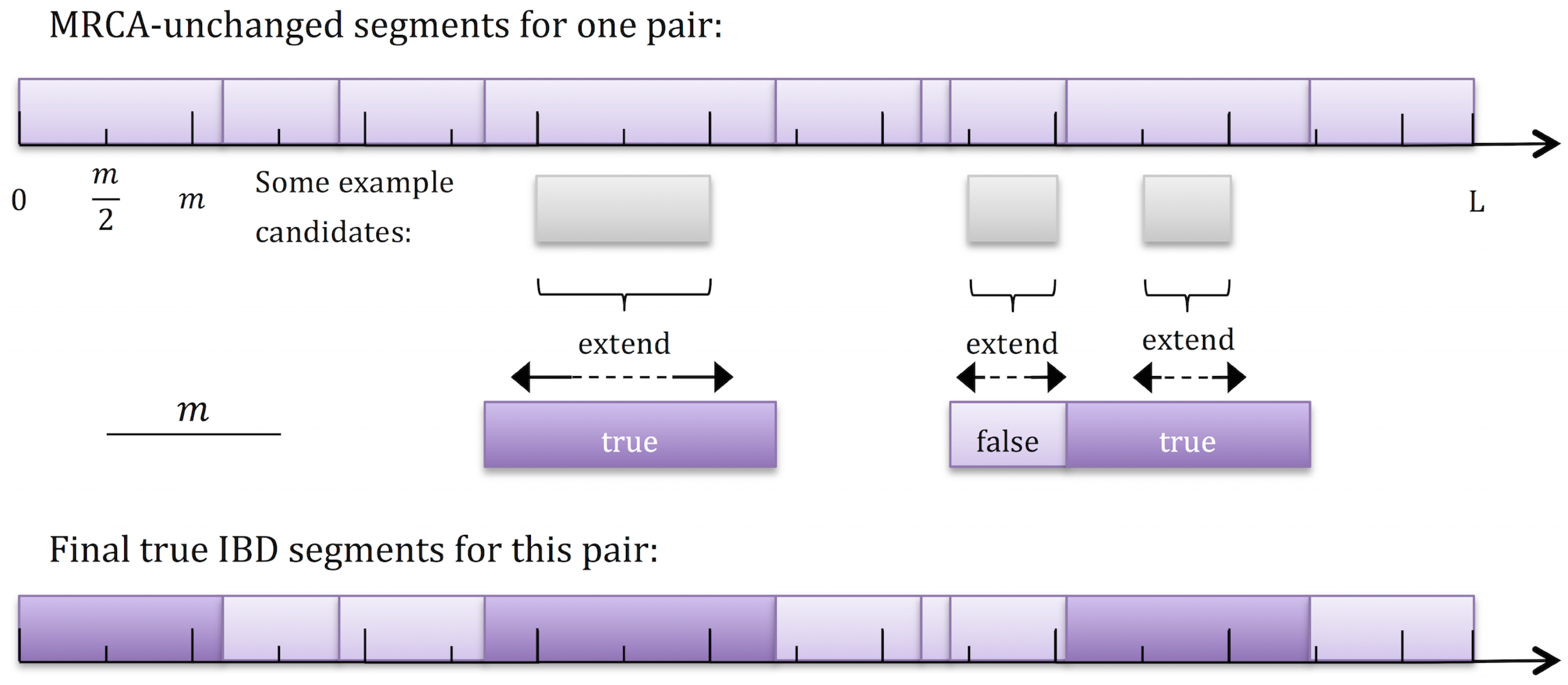
A two-step approach for IBD segment discovery. For a given pair of individuals, a partition of the chromosome into shared segments is shown at the top, where in each segment, the MRCA is unchanged. Tickmarks are shown at multiples of m/2, and segments that span at least two tickmarks are considered for further validation. Note that segments that span just a single tickmark are necessarily shorter than m. Extension of some of the candidate segments is shown below the chromosome. The partition of the chromosome at the bottom highlights IBD segments longer than m.

Algorithm 2:

Two-Step Algorithm

TwoStep({T_i}, {x_i})

1 for each (u,v)

2 PrevLCA[u, v] = LCA of u and v in T₀, LastChanged[u, v] = 0

3 s = m/2, Candidates = ∅, x = 0, b = 0

4 Preprocess all trees for LCA

5 while x < L

6 get (T_i, x_i), where i is the maximal index such that x_i < x + s

7 for each (u, v)

8 CurrLCA[u, v] = LCA of u and v in T_i

9 if CurrLCA[u, v] = = PrevLCA[u, v] // (u, v) is a candidate in block b

10 Candidates[b] = Candidates[b] ∪ (u, v)

11 PrevLCA[u, v] = CurrLCA[u, v]

12 if b > 0

13 IBDSearch(Candidates, b, Interval)

14 Interval = (x, x_i)

15 x = x_i, b = b + 1

16 IBDSearch(Candidates, b, Interval) // Process segments that end at L

IBDSearch(Candidates, b, Interval)

1 CL = Candidates[b − 2], CC = Candidates[b − 1], CR = Candidates[b]

2 get T_i where x_i = = Interval.start

3 for each (u, v)

4 PrevLCA[u, v] = LCA of u and v in T_i

5 for (u, v)∈CL and not in CC // Determine right boundary of segment in CL

6 for each (T_j, x_j) with x_j∈Interval

7 CurrLCA[u, v] = LCA of u and v in T_j

8 if CurrLCA[u, v] ≠ PrevLCA[u, v]

9 if x_j–LastChanged[u, v] > m

10 report((u, v), [LastChanged[u, v], x_j])

11 break

12 for (u, v)∈CR and not in CC // Determine left boundary of segment in CR

13 for each (T_j, x_j) with x_j∈Interval in reverse order

14 CurrLCA[u, v] = LCA of u and v in T_j

15 if CurrLCA[u, v] ≠ PrevLCA[u, v]

16 LastChanged[u, v] = x_j₊₁

17 break

18 for (u, v)∈CC // inner-segment validation

19 for each (T_j, x_j) with x_j∈Interval

20 CurrLCA[u, v] = LCA of u and v in T_j

21 if CurrLCA[u, v] ≠ PrevLCA[u, v]

22 if x_j–LastChanged[u, v] > m

23 report((u, v), [LastChanged[u, v], x_j])

24 LastChanged[u, v] = x_j

25 PrevLCA[u, v] = CurrLCA[u, v]

The running time of the candidate identification step is simply \documentclass{aastex}\usepackage{amsbsy}\usepackage{amsfonts}\usepackage{amssymb}\usepackage{bm}\usepackage{mathrsfs}\usepackage{pifont}\usepackage{stmaryrd}\usepackage{textcomp}\usepackage{portland, xspace}\usepackage{amsmath, amsxtra}\pagestyle{empty}\DeclareMathSizes{10}{9}{7}{6}\begin{document} $$O \left( \frac { L } { m } n^2 \right)$$ \end{document} . The running time of the validation step depends on the number of candidates. The average number of pairs of candidates when comparing two trees at distance m/2 apart is, from population genetic theory and for mN ≫ 1, approximately (mN)⁻¹ (Simonsen and Churchill, 1997). We therefore expect \documentclass{aastex}\usepackage{amsbsy}\usepackage{amsfonts}\usepackage{amssymb}\usepackage{bm}\usepackage{mathrsfs}\usepackage{pifont}\usepackage{stmaryrd}\usepackage{textcomp}\usepackage{portland, xspace}\usepackage{amsmath, amsxtra}\pagestyle{empty}\DeclareMathSizes{10}{9}{7}{6}\begin{document} $$O \left( \frac { n^2 } { mN } \right)$$ \end{document} candidate pairs of individuals per tickmark, and \documentclass{aastex}\usepackage{amsbsy}\usepackage{amsfonts}\usepackage{amssymb}\usepackage{bm}\usepackage{mathrsfs}\usepackage{pifont}\usepackage{stmaryrd}\usepackage{textcomp}\usepackage{portland, xspace}\usepackage{amsmath, amsxtra}\pagestyle{empty}\DeclareMathSizes{10}{9}{7}{6}\begin{document} $$O \left( \frac { L } { m } \times \frac { n^2 } { mN } \right)$$ \end{document} candidates overall. Each such candidate requires a comparison of the tMRCA between O (Nm log n) trees for its IBD status to be determined. Preprocessing all trees for LCA (in time O(n) for each tree), will require overall time O (NLn log n). Since each LCA query takes constant time, the combined LCA query time will be \documentclass{aastex}\usepackage{amsbsy}\usepackage{amsfonts}\usepackage{amssymb}\usepackage{bm}\usepackage{mathrsfs}\usepackage{pifont}\usepackage{stmaryrd}\usepackage{textcomp}\usepackage{portland, xspace}\usepackage{amsmath, amsxtra}\pagestyle{empty}\DeclareMathSizes{10}{9}{7}{6}\begin{document} $$O \left( \frac { L } { m } \times \frac { n^2 } { mN } \times Nm \log n \right) = O \left( \frac { L } { m } n^2 \log n \right)$$ \end{document} . Note that this is asymptotically larger than the time of the candidate extraction step \documentclass{aastex}\usepackage{amsbsy}\usepackage{amsfonts}\usepackage{amssymb}\usepackage{bm}\usepackage{mathrsfs}\usepackage{pifont}\usepackage{stmaryrd}\usepackage{textcomp}\usepackage{portland, xspace}\usepackage{amsmath, amsxtra}\pagestyle{empty}\DeclareMathSizes{10}{9}{7}{6}\begin{document} $$\Big(O \left( \frac { L } { m } n^2 \right)\Big)$$ \end{document} . The overall time complexity is therefore \documentclass{aastex}\usepackage{amsbsy}\usepackage{amsfonts}\usepackage{amssymb}\usepackage{bm}\usepackage{mathrsfs}\usepackage{pifont}\usepackage{stmaryrd}\usepackage{textcomp}\usepackage{portland, xspace}\usepackage{amsmath, amsxtra}\pagestyle{empty}\DeclareMathSizes{10}{9}{7}{6}\begin{document} $$O \left( \frac { L } { m } n^2 \log n + NLn \log n \right)$$ \end{document} , which is O (n² log n) assuming N = O(n) and considering L and m as constants.

3.4. A discretized two-step approach with a novel candidate extraction algorithm

Let us now analyze the complexity of the two-step approach when segment lengths are discretized. The time spent on candidate extraction remains \documentclass{aastex}\usepackage{amsbsy}\usepackage{amsfonts}\usepackage{amssymb}\usepackage{bm}\usepackage{mathrsfs}\usepackage{pifont}\usepackage{stmaryrd}\usepackage{textcomp}\usepackage{portland, xspace}\usepackage{amsmath, amsxtra}\pagestyle{empty}\DeclareMathSizes{10}{9}{7}{6}\begin{document} $$O \left( \frac { L } { m } n^2 \right)$$ \end{document} , but preprocessing and verification now take \documentclass{aastex}\usepackage{amsbsy}\usepackage{amsfonts}\usepackage{amssymb}\usepackage{bm}\usepackage{mathrsfs}\usepackage{pifont}\usepackage{stmaryrd}\usepackage{textcomp}\usepackage{portland, xspace}\usepackage{amsmath, amsxtra}\pagestyle{empty}\DeclareMathSizes{10}{9}{7}{6}\begin{document} $$O \left( \frac { L } { m } \times \left( n + \frac { n^2 } { mN } \right) \times \frac { m } { d } \right)$$ \end{document} , which is \documentclass{aastex}\usepackage{amsbsy}\usepackage{amsfonts}\usepackage{amssymb}\usepackage{bm}\usepackage{mathrsfs}\usepackage{pifont}\usepackage{stmaryrd}\usepackage{textcomp}\usepackage{portland, xspace}\usepackage{amsmath, amsxtra}\pagestyle{empty}\DeclareMathSizes{10}{9}{7}{6}\begin{document} $$O \left( \frac { Ln } { d } \times \left( 1 + \frac { n } { mN } \right) \right)$$ \end{document} compared to \documentclass{aastex}\usepackage{amsbsy}\usepackage{amsfonts}\usepackage{amssymb}\usepackage{bm}\usepackage{mathrsfs}\usepackage{pifont}\usepackage{stmaryrd}\usepackage{textcomp}\usepackage{portland, xspace}\usepackage{amsmath, amsxtra}\pagestyle{empty}\DeclareMathSizes{10}{9}{7}{6}\begin{document} $$O \left( L \log n \left( nN + \frac { n^2 } { m } \right) \right)$$ \end{document} when considering all trees. Assuming m, L, and d are constants and N = O(n), the overall complexity is quadratic, O (n²). While this is asymptotically no better than the discretized naïve algorithm (section 3.2), the complexity bottleneck for the discretized two-step approach is the candidate extraction stage, which we now seek to improve. Our novel algorithm relies on the following intuitive observation.

Observation 1 The MRCA, a, of a pair of leaves l, r in the respective subtrees spanned by the two children of a at locus x persists across to locus \documentclass{aastex}\usepackage{amsbsy}\usepackage{amsfonts}\usepackage{amssymb}\usepackage{bm}\usepackage{mathrsfs}\usepackage{pifont}\usepackage{stmaryrd}\usepackage{textcomp}\usepackage{portland, xspace}\usepackage{amsmath, amsxtra}\pagestyle{empty}\DeclareMathSizes{10}{9}{7}{6}\begin{document} $$x^ { \prime } = x + \frac { m } { 2 } $$ \end{document} , if and only if

– a is a node at x′, and

– l, r are leaves in respective subtrees spanned by the two children of a at x′.

The practical implication of Observation 1 is that we should look for a triple intersection between successive trees: an ancestor, a leaf in its left subtree, and a leaf in its right subtree. We implement this intersection by hashing all ancestors in the two trees and looking for shared ones, followed by determining which pairs of leaves are found, in both trees, in distinct subtrees that descend from the shared ancestor. The newly developed algorithm is illustrated in Fig. 4 (see pseudocode in Yang, 2014).

FIG. 4.

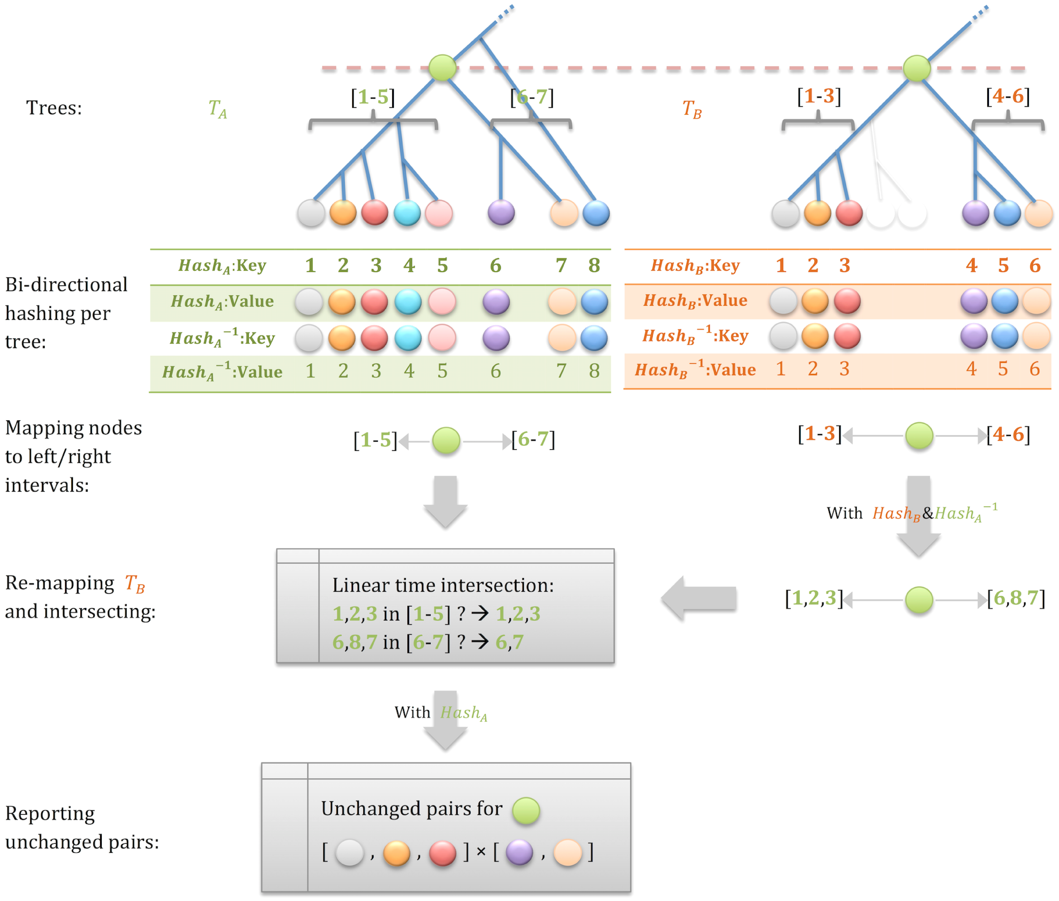
Intersecting trees using hashing. We perform an in-order traversal of each tree in linear time, while hashing all internal nodes, bidirectionally hashing all leaves, and mapping left and right intervals along the traversal order for each internal node. The hash and reverse-hash tables enable us to compute the intersection between the intervals of corresponding internal nodes of the two trees in linear time. Doing that for the left and right children of an ancestor yields the pairs of leaves for which the MRCA is unchanged between the two trees.

In-order traversal and hashing the internal nodes takes O(n) time, and finding the triple intersection can be done, for each internal node, in linear time using bidirectional hashing of the leaves. The overall time complexity is dominated by the number of potential shared ancestors (O(n)) times the number of leaves descending from each ancestor (O(n)) and is thus, at the worst case, O (n²). However, coalescent genealogies are asymptotically balanced (Li and Wiehe, 2013), and it is easy to show that for a full tree topology, the complexity is O (n log n) (see also Supplementary Fig. S2). With an O (n log n) algorithm to extract candidate pairs, the total time complexity, assuming N = O(n), becomes O (n log n), and this is our presently best theoretical result.

4. Benchmarking

We implemented the algorithms of section 3 in C/C++ and performed experiments to evaluate their practical running time. Testing was conducted on a standard workstation running Ubuntu 10.04 LTS. Figure 5 compares the wallclock running time of different algorithms. As a previous implementation of the naïve algorithm was based on the Python open source library DendroPy (Browning and Browning, 2013), results for that method are also shown. While the two-step approach is asymptotically superior, the LCA running time has a large prefactor compared to the tight implementation of the naïve algorithm, and it becomes faster only around n ≈ 7000.

FIG. 5.

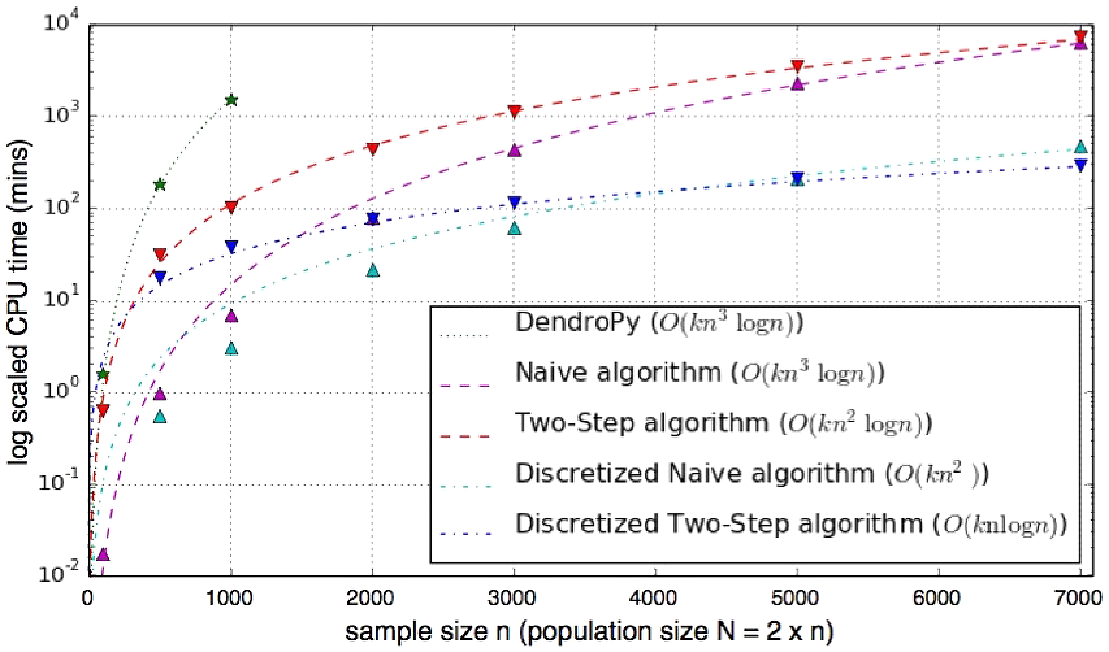
Running times of the algorithms considered in this study (symbols). In all experiments, we used fastsimcoal2 (Excoffier and Foll, 2011) to generate the ARGs, N = 2n, L = 1M, and m = 0.01M. When discretizing segment lengths, we used ε = 0.01. Lines are fits to the asymptotic running times (see boxed key).

5. Applications: Evaluating Demographic Parameters

In this section we show some examples of using our method for demographic inference of recent population history. We developed a tool that uses a new statistic of total IBD to infer demography and demonstrate the process of evaluating feasibility and accuracy of such analysis.

5.1. Population models and IBD statistics used

We first aim at evaluating the effectiveness of the new IBD statistic for inference. We thus start from very simple models, the constant population size model (parameterized by N) and the bottleneck model (parameterized by NA, NC, NB, T, and TB; see Fig. 6 for detailed explanation of the models and the parameters). The latter model is expressive enough to be consistent with some populations that went through a sharp decline in population size in recent history (Palamara et al., 2012; Gusev et al., 2012; Carmi et al., 2014a; Lim et al., 2014; Gauvin et al., 2014).

FIG. 6.

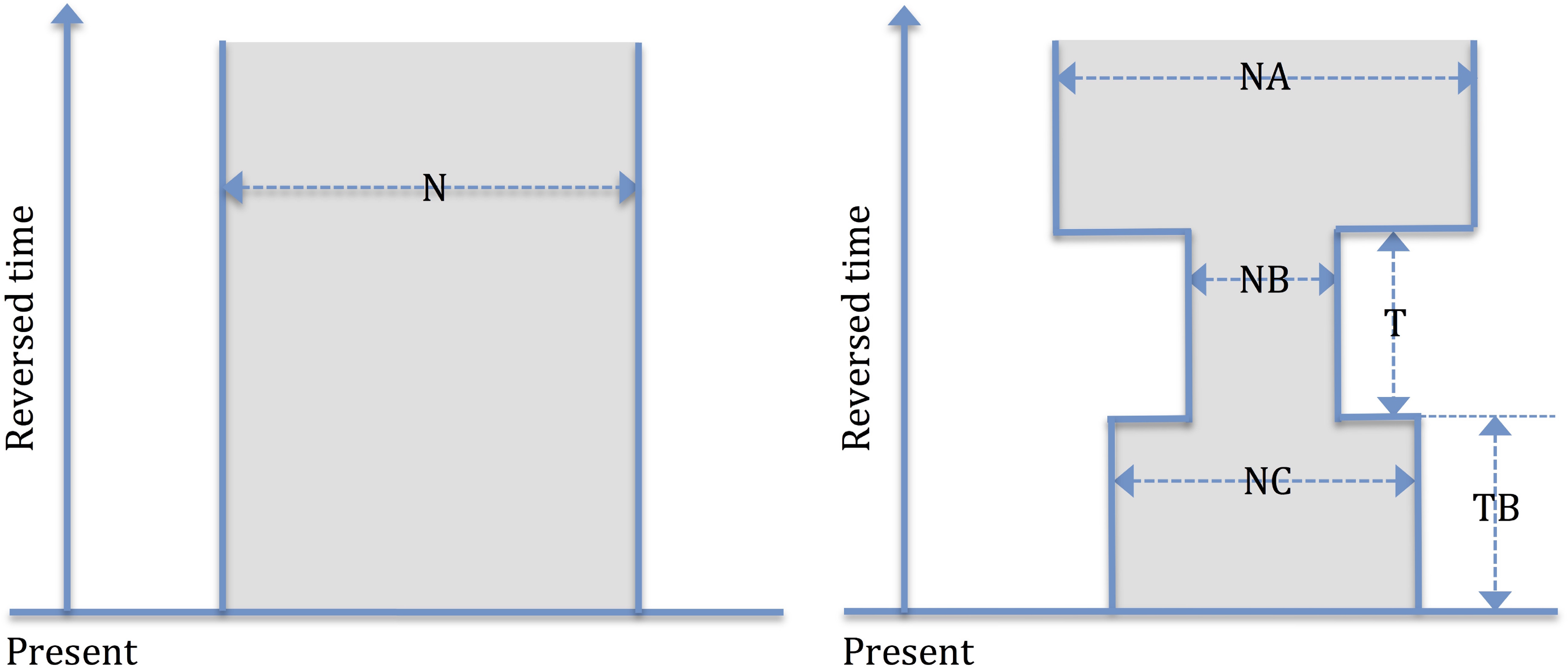
Simple demographic models. The left panel depicts a naive model of constant population size, and the right one depicts a more complicated and realistic bottleneck model, which involves recent population shrinkage. The time axis goes top to bottom. The constant size population model is parameterized by N (effective population size); the bottleneck model is parameterized by NA (ancient population size), NC (current population size), NB (bottleneck population size), T (bottleneck duration), and TB (time length to bottleneck event).

Figure 7 plots the statistic we use for inference, average total IBD-sharing across the cohort, for several constant population sizes across different cohort sizes and cutoffs m for IBD length. The decay pattern of this statistic as m increases and its growth, with accumulated reference genomes are both encoded as a matrix of total IBD statistics for different values of these two coordinates, which provides some information about the model parameters (see Palamara et al., 2012; Palamara and Pe'er, 2013; Carmi et al., (2014a,b). As shown in Figure 7, the value of model parameter N gives rise to a unique value of this IBD statistic, which suggests that it is possible to estimate this parameter based on the observed IBD statistics. Also, the developments in earlier sections of this manuscript allow using this statistic for demographic inference.

FIG. 7.

Total-sharing statistics for different population size parameters under constant population size model. Each statistic is constructed by all the points in a surface, which is indexed by the number of reference genomes i and the IBD cutoff value m. For a specific point in (i, m), the value of the statistic represents the average total fraction of IBD sharing of one genome against i other genomes where IBD cutoff value is m.

The practical inference process is as follows: We simulate data for different values of the studied parameter using the fastsimcoal2 simulator (Excoffier and Foll, 2011) and extract IBD segments with our designed tool; we tally total IBD statistics (average total IBD-sharing across the cohort, discussed in the above paragraph; also see Fig. 7) from these data, and we use 1000 replicates for one statistic under each parameter combination, which is necessary and enough to get a better quantification of the statistic (a stable or converged value of the statistic); we calculate the distance (sum of the squared differences) between the matrix of statistics for the designated “true” population parameter and those of all other guessed parameters. Ideally, the distance would be minimized at the “true” parameter, supporting single-point estimation for that parameter. In practice, when no ground truth solution is available, we will use the distance of the simulated statistics from the empirical matrix for real data instead of the true matrix. Figure 8 shows such measurement under constant population size model when we treat different N's as real parameters. In the next section, we will expand this evaluation to all parameters in bottleneck model.

FIG. 8.

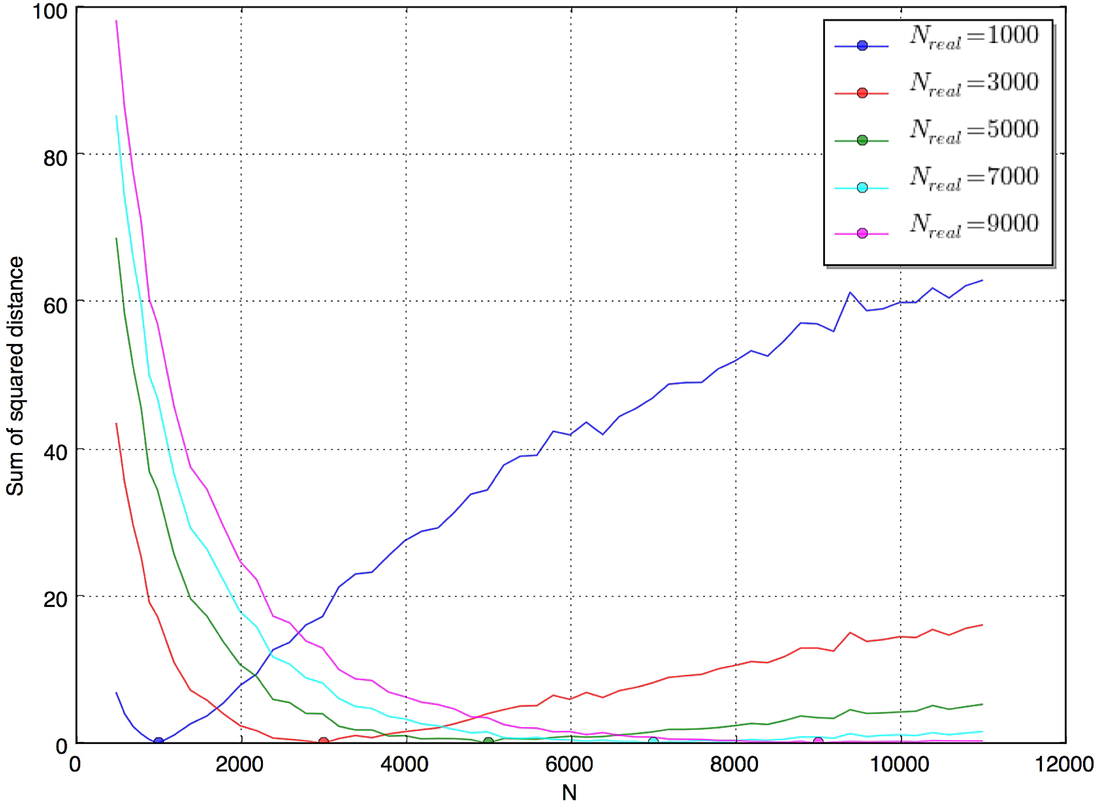
The distance curve under a constant population size model where the true parameter is set to different values. We can see the minimum distance is always attained at the true value (though inaccurate for large N), which means the total IBD statistic allows good estimation of this population parameter.

5.2. Results for the bottleneck model

In this section we present a single-point evaluation under the bottleneck model. This model requires five parameters to be estimated: NC, NA, NB, T, and TB. Their default values are set to NA = 10,000, NC = 1000, NB = 200, T = 10, TB = 30. We evaluated all of them, but focus the discussion on NB and T, which we find to be most instructive (see Supplementary Fig. S3, Fig. S4, and Fig. S5 for the results regarding NA, NC, and TB). We computed the joint distance surface for NB and T (see Fig. 9). We observed that individual values of NB and T are nearly indistinguishable in terms of total sharing, but there is a line across the joint plane that always achieves the minimum distance. This indicates that the ratio \documentclass{aastex}\usepackage{amsbsy}\usepackage{amsfonts}\usepackage{amssymb}\usepackage{bm}\usepackage{mathrsfs}\usepackage{pifont}\usepackage{stmaryrd}\usepackage{textcomp}\usepackage{portland, xspace}\usepackage{amsmath, amsxtra}\pagestyle{empty}\DeclareMathSizes{10}{9}{7}{6}\begin{document} $$ \frac { T } { NB } $$ \end{document} determines the best-fit model rather than the individual values of NB and T. A better parameterization for NB and T is thus f and NB, where \documentclass{aastex}\usepackage{amsbsy}\usepackage{amsfonts}\usepackage{amssymb}\usepackage{bm}\usepackage{mathrsfs}\usepackage{pifont}\usepackage{stmaryrd}\usepackage{textcomp}\usepackage{portland, xspace}\usepackage{amsmath, amsxtra}\pagestyle{empty}\DeclareMathSizes{10}{9}{7}{6}\begin{document} $$f = \frac { T } { NB } $$ \end{document} is the bottleneck strength to which total IBD is very sensitive.

FIG. 9.

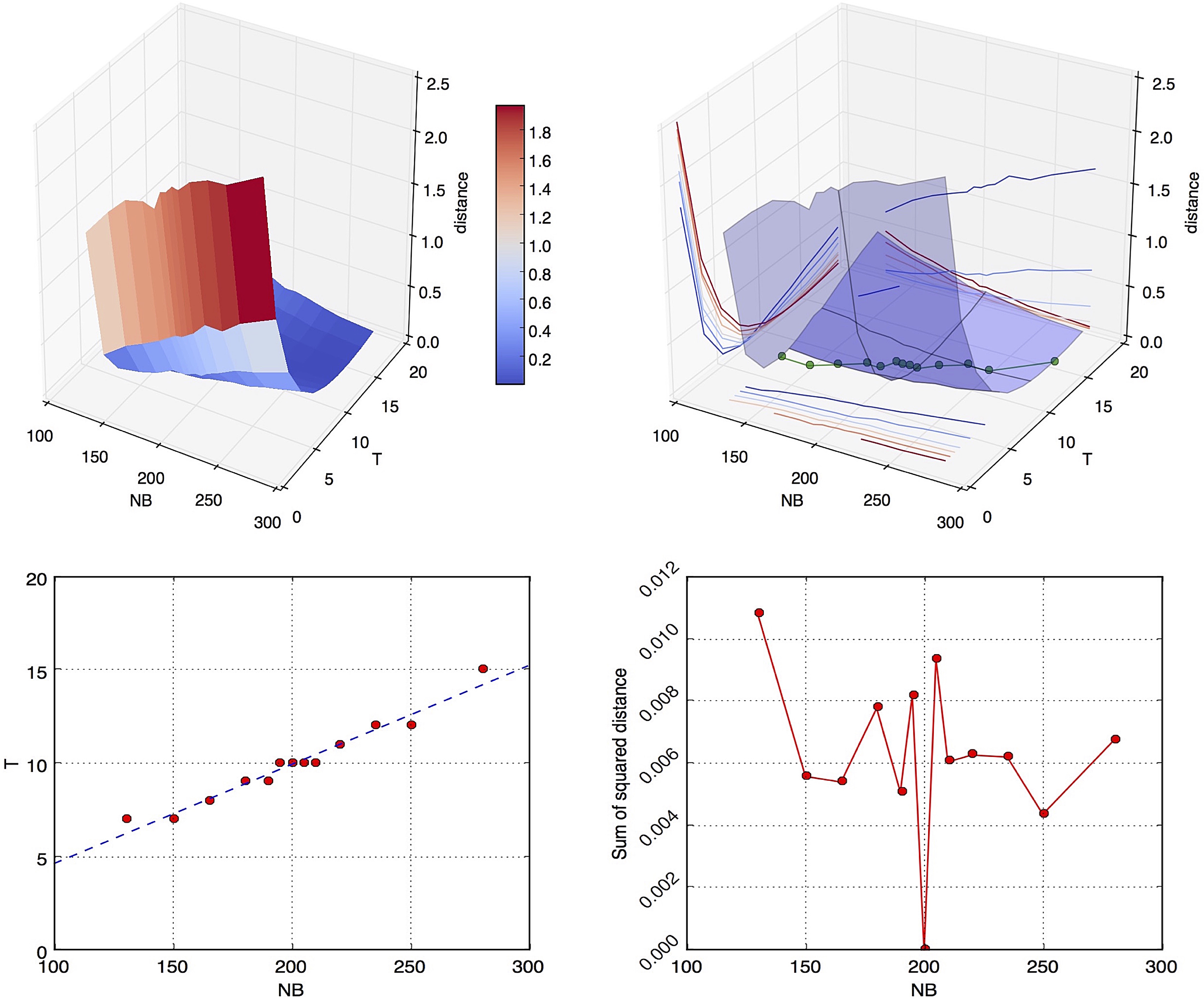
The top two figures are renderings of the joint distance surface for NB and T given all other three correct parameters, NA, NC, and TB, where the true values are NB_real = 200,T_real = 10. The points that attain the minimum distance are highlighted in green (top right). A linear-fit of only these minima (bottom left) is T = 0.053 × NB − 0.651, where the slope is very close to the true ratio of T and NB 0.05. The distances attained along the linear fit (bottom right) approach zero and give a sense of the noise level around the convex pattern.

The reasoning above allows evaluating feasibility of inferring distinct model parameters from total sharing statistics. We fit all these parameters to statistics from real data by a grid search. We experimented also with some faster optimization algorithms, both derivative-based, such as L-BFGS-B algorithm (Byrd et al., 1995), as well as non-derivative-based ones, such as Nelder-Mead algorithm (Nelder and Mead, 1965). Unfortunately, we report (data not shown) that these are ineffective for this problem due to instability across any of the specific dimensions of the problem. Specifically, the statistic used in the inference is simulated. In that case, the distance curve (or surface) we get from the statistics will be fluctuant all the time (as the statistics have no perfectly stable or converged values from finite replicates of simulations), thus unable to make these classical optimizers successfully optimize along.

6. Discussion

We designed and implemented a set of efficient algorithms for extraction of ground-truth IBD segments from a sequence of coalescent trees. We anticipate our method to facilitate progress across multiple areas of IBD research. First, extraction of IBD segments from simulated ARGs will inform analysis of methods based on the increasingly popular SMC and SMC¹ models (e.g., Harris and Nielsen, 2013; Li and Durbin, 2011). Second, while simulation-based approaches for demographic inference are widespread (Beaumont et al., 2002; Excoffier et al., 2013), no existing method is based on IBD sharing, which is highly informative regarding recent history. Our method will provide the community with the enabling tool for such analysis. Finally, an efficient means to generate ground-truth-simulated IBD data will enable researchers to generate a background null distribution of key IBD statistics, against which alternative hypothesis can be tested, such as positive natural selection (Albrechtsen et al., 2010) or genetic association (Gusev et al., 2011).

The coalescent trees (or ARGs) that are our input are often simulated, raising the possibility of replacing the benefits of our work by simulators that directly report IBD segments. However, even if simulators evolve to directly output IBD segments, the most straightforward path will be to include methods such as ours as a feature. Additionally, ARGs not only are, but will likely continue to be, the standard output of simulators, as they concisely report all relevant information about the genetic ancestry of the sample, so our method will likely be needed even as simulators evolve. We further point out that the empirical results have demonstrated that the utility of our new two-step approach is limited to sample sizes in the thousands. However, the fast decline in the cost of sequencing and the rapid growth in the number of available genomes generate demand for ever larger simulated samples, where our two-step algorithm is competitive.

The latter part of the article includes demonstration of the utility of our tool for demographic inference via total IBD sharing. We evaluated this new statistic across some simple models and showed the potential of our tool to be used broadly in the community for this type of analysis. This evaluation raises two issues worthy of future work. First, the need to evaluate many unknown parameters jointly, rather than pursue single-point estimation, is a weakness of this strategy. Potential improvement may rely on the ability to break up the set of parameters to low-dimension subsets that can each be optimized separately. The second issue has to do with the reliance of our parameterized models on specific model assumption, which often oversimplify realistic historical scenarios. More flexible models, for example with arbitrary population size at each generation, that rely on regularization rather than a limited number of parameters are an attractive strategy to tackle this issue in the future.

Footnotes

Acknowledgment

We thank the Human Frontier Science Program (SC) and NIH grant 1R01MH095458-01A1 (IP).

Author Disclosure Statement

No competing financial interests exist.

References

Albrechtsen

, Moltke

, and Nielsen

2010. Natural selection and the distribution of identity-by-descent in the human genome. Genetics, 186, 295–308.

Beaumont

M.A.

, and Farach-Colton

2000. The LCA problem revisited, pp. 88–94. In Proceedings of the 4th Latin American Symposium on Theoretical Informatics, LATIN ’00. London, 2000. Springer-Verlag, London.

Beaumont

M.A.

, Zhang

, and Balding

D.J.

2002. Approximate Bayesian computation in population genetics. Genetics, 162, 2025–2035.

Berkman

, Galil

, Schieber

, and Vishkin

1989. Highly parallelizable problems, pp. 309–319. In Proceedings of the Twenty-first Annual ACM Symposium on Theory of Computing, STOC ’89. New York, NY. ACM, New York.

Browning

B.L.

, and Browning

S.R.

2011. A fast, powerful method for detecting identity by descent. Am. J. Hum. Genet. 88, 173–182.

Browning

B.L.

, and Browning

S.R.

2013. Detecting identity by descent and estimating genotype error rates in sequence data. Am. J. Hum. Genet., 93, 840–851.

Byrd

R.H.

, Lu

, Nocedal

, and Zhu

1995. A limited memory algorithm for bound constrained optimization. SIAM J. Sci. Comput., 16, 1190–1208.

Carmi

, Francesco Palamara

, Vacic

, et al. 2013. The variance of identity-by-descent sharing in theWright-Fisher model. Genetics, 193, 911–928.

Carmi

, Hui

K.Y.

, Kochav

, et al. 2014a. Sequencing an ashkenazi reference panel supports population-targeted personal genomics and illuminates Jewish and European origins. Nat. Commun., 5, 4835.

10.

Carmi

, Wilton

P.R.

, Wakeley

, and Pe'er

2014b. A renewal theory approach to IBD sharing. Theor. Popul. Biol., 97, 35–48.

11.

Chiang

C.W.K.

, Ralph

, and Novembre

2014. Conations of short IBD blocks can bias inferred length of IBD.

12.

Conrad

D.F.

, Jakobsson

, Coop

, et al. 2006. A worldwide survey of haplotype variation and linkage disequilibrium in the human genome. Nat. Genet., 38, 1251–1260.

13.

Excoffier

, and Foll

2011. fastsimcoal: A continuous-time coalescent simulator of genomic diversity under arbitrarily complex evolutionary scenarios. Bioinformatics, 27, 1332–1334.

14.

Excoffier

, Dupanloup

, Huerta-Sánchez

, et al. 2013. Robust demographic inference from genomic and SNP data. PLoS Genet. 9, e1003905.

15.

Fearnhead

, and Donnelly

2001. Estimating recombination rates from population genetic data. Genetics, 159, 1299–1318.

16.

Gauvin

, Moreau

, Lefebvre

J.-F.

, et al. 2014. Wide patterns of identity-by-descent sharing in the french canadian founder population. Eur. J. Hum. Genet., 22, 814–821.

17.

Griffiths

R.C.

, and Marjoram

1996. Ancestral inference from samples of DNA sequences with recombination. J. Comput. Biol., 3, 479–502.

18.

Griffiths

R.C.

, and Marjoram

1997. An ancestral recombination graph, pp. 257–270. In Donnelly

, and Tavaré

, eds. Progress in Population Genetics and Human Evolution (IMA Volumes in Mathematics and its Applications), volume 87. Springer-Verlag, Berlin.

19.

Guha

, Rosenfeld

J.A.

, Malhotra

A.K.

, et al. 2012. Implications for health and disease in the genetic signature of the Ashkenazi Jewish population. Genome Biol. 13, R2.

20.

Gusev

, Kenny

E.E.

, Lowe

J.K.

, et al. 2011. DASH: A method for identical-by-descent haplotype mapping uncovers association with recent variation. Am. J. Hum. Genet., 88, 706–717.

21.

Gusev

, Lowe

J.K.

, Stoffel

, et al. 2009. Whole population, genome-wide mapping of hidden relatedness. Genome Res. 19, 318–326.

22.

Gusev

, Palamara

P.F.

, Aponte

, et al. 2012. The architecture of longrange haplotypes shared within and across populations. Mol. Biol. Evol. 29, 473–486.

23.

Harris

, and Nielsen

2013. Inferring demographic history from a spectrum of shared haplotype lengths. PLoS Genet. 9, e1003521.

24.

Henn

B.M.

, Cavalli-Sforza

L.L.

, and Feldman

M.W.

2012a. The great human expansion. Proc. Natl. Acad. Sci. USA, 109, 17758–17764.

25.

Henn

B.M.

, Hon

, Macpherson

J.M.

, et al. 2012b. Cryptic distant relatives are common in both isolated and cosmopolitan genetic samples. PLoS One, 7, e34267.

26.

Hudson

R.R.

1983. Properties of a neutral allele model with intragenic recombination. Theor. Popul. Biol., 23, 183–201.

27.

Hudson

R.R.

1990. Gene genealogies and the coalescent process. Oxford Surv. Evol. Biol. 7, 44.

28.

Huff

C.D.

, Witherspoon

D.J.

, Simonson

T.S.

, et al. 2011. Maximum-likelihood estimation of recent shared ancestry (ERSA). Genome Res. 21, 768–774.

29.

, and Durbin

2011. Inference of human population history from individual whole-genome sequences. Nature, 475, 493–496.

30.

, and Wiehe

2013. Coalescent tree imbalance and a simple test for selective sweeps based on microsatellite variation. PLoS Comput. Biol. 9, e1003060.

31.

Liang

, Zöllner

, and Abecasis

G.R.

2007. GENOME: a rapid coalescent-based whole genome simulator. Bioinformatics, 23, 1565–1567.

32.

Lim

E.T.

, Wrtz

, Havulinna

A.S.

, et al., for the Sequencing Initiative Suomi (SISu) Project. 2014. Distribution and medical impact of loss-of-function variants in the Finnish founder population. PLoS Genet. 10, e1004494.

33.

Marjoram

, and Wall

2006. Fast “coalescent” simulation. BMC Genet. 7, 16.

34.

Mathieson

, and McVean

2014. Demography and the age of rare variants. PLoS Genet. 10, e1004528.

35.

McVean

G.A.T.

, and Cardin

N.J.

2005. Approximating the coalescent with recombination. Philos. T. Roy. Soc. B., 360, 1387–1393.

36.

Nelder

J.A.

, and Mead

1965. A simplex method for function minimization. Comp. J., 7, 308–313.

37.

Palamara

P.F.

, and Pe'er

2013. Inference of historical migration rates via haplotype sharing. Bioinformatics, 29, 180–188.

38.

Palamara

P.F.

, Lencz

, Darvasi

, and Pe'er

2012. Length distributions of identity by descent reveal fine-scale demographic history. Am. J. Hum. Genet. 91, 809–822.

39.

Ralph

, and Coop

2013. The geography of recent genetic ancestry across Europe. PLoS Biol. 11, e1001555.

40.

Schaffner

S.F.

, Foo

, Gabriel

, et al. 2005. Calibrating a coalescent simulation of human genome sequence variation. Genome Res. 15, 1576–1583.

41.

Simonsen

K.T.

, and Churchill

G.A.

1997. A Markov chain model of coalescence with recombination. Theor. Popul. Biol. 52, 43–59.

42.

S.-Y.

, Kasberger

, Baranzini

, et al. 2012. Detection of identity by descent using nextgeneration whole genome sequencing data. BMC Bioinform. 13, 121.

43.

Tataru

, Nirody

J.A.

, and Song

Y.S.

2014. diCal–IBD: Demography-aware inference of identity-by-descent tracts in unrelated individuals. Bioinformatics, 30, 3430–3431.

44.

The Wellcome Trust Case Control Consortium. 2007. Genome-wide association study of 14,000 cases of seven common diseases and 3,000 shared controls. Nature, 447, 661–678.

45.

Wakeley

2005. Coalescent Theory, An Introduction. Roberts and Company, Greenwood Village, CO.

46.

Wiuf

, and Hein

1999. Recombination as a point process along sequences. Theor. Popul. Biol. 55, 248–259.

47.

Yang

2014. IBDdetection. https://github.com/morrisyoung/IBDdetection

48.

Zhang

Q.S.

, Browning

B.L.

, and Browning

S.R.

2015. Genome-wide haplotypic testing in a Finnish cohort identifies a novel association with low-density lipoprotein cholesterol. Eur. J. Hum. Genet. 23, 672–677.

Supplementary Material

Please find the following supplemental material available below.

For Open Access articles published under a Creative Commons License, all supplemental material carries the same license as the article it is associated with.

For non-Open Access articles published, all supplemental material carries a non-exclusive license, and permission requests for re-use of supplemental material or any part of supplemental material shall be sent directly to the copyright owner as specified in the copyright notice associated with the article.

0.00 MB

1.74 MB