Cell division is a key biological process in which cells divide forming new daughter cells. In the present study, we investigate continuously how a Coleochaete cell divides by introducing a modified differential equation model in parametric equation form. We discuss both the influence of “dead” cells and the effects of various end-points on the formation of the new cells' boundaries. We find that the boundary condition on the free end-point is different from that on the fixed end-point; the former has a direction perpendicular to the surface. It is also shown that the outer boundaries of new cells are arc-shaped. The numerical experiments and theoretical analyses for this model to construct the outer boundary are given.
1. Introduction
How does cell shape affect cell division? There has been some conjecture about this problem, but there is no completely theoretical result found.
More than 100 years ago, plant biologists believed that the majority of plant cell division orientation can be predicted by their shape. In 1863, W. Hofmeister noted that the new cell wall is usually perpendicular to the expanding on the main axis of the cells and forms in a plane, that is, perpendicular to the long axis of the cell. In 1888, Léo Errera said most of the cell wall of the plant cell division usually follows the shortest path rules (smith, 2001), often referred to as Errera's rule. Many experimental results support the claim. While there are some important findings, such as E.W. Sinnott and R. Bloch (1940) pointed out that cell split has the phenomenon of radial division.
Due to the characteristics of Coleochaete, it is used as an example to study the mechanism of plant cell division. The growth of this kind of cell is slow and also relatively “simple.” Coleochaete itself plays a very important role in plant research and is usually considered one of the most evolved species of green algae, and the studies on the evolutionary origin of land plants often refer to it (Graham, 1984; Timme and Delwiche, 2010).
Recently, Dupuy et al. (2010) and Besson and Dumais (2011) showed that the selection of plane of division involves a competition between alternative configurations whose geometries represent local area minima. They used the variational method to derive the condition that the new cell wall satisfies and found the relationship between the new wall and original outer membrane. They also used the statistical mechanism to analyze the image formation. This is a very innovative discovery, and their achievement was well reviewed by Prusinkiewicz (2011).
What is the relationship between cell division and some classical mathematical problems? There is a geometrical problem named “regional segmentation,” which is closely related to the classical isoperimetric problem. This problem was initially raised by Wiener (1914). By using geometric methods, Wiener proved that “the shortest line passing through two given points on the boundary of a given circle, dividing the area of the circle in a given ratio, is an arc of a circle.” Goldberg (1969) presented a general problem: Given a convex quadrilateral, find the shortest curve that divides it into two equal areas. This problem is still unsolved. In 1973, Richard Joss announced that he had proved it. However, Klamkin (1992) wrote: “Since Joss' proof has not been published, it should still be considered as an open problem.”
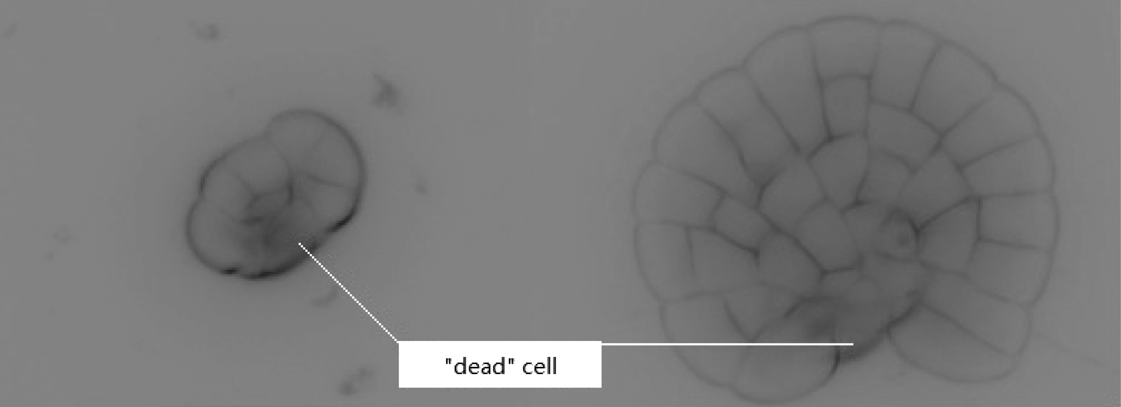
Shi and Wang (2012) had discussed the nonuniform division in which there is a “dead” cell, but they showed no theoretical analysis. A cell is called a dead cell if it keeps its size fixed and without division (Fig. 1). They gave a mathematical simulation of Coleochaete cell division process from the perspective of image simulation, mathematical morphology, and Chan-Vese active contour model for image processing and image fusion method, but they provided no mechanism analysis.
Cell-expanding pictures at 48 hours and 208 hours.
Motivated by the work of Besson and Dumais (2011), Wang et al. (2015) tried to establish a link between geometry and plant cell. They gave a model in the form of parametric equation to describe dividing flat domains with more complex boundaries, especially for some nonconvex domains. The equation system and their boundary value conditions in the model are consistent with the Cartesian coordinate form by Besson and Dumais (2011). Geometrically, this model can be used to find the solution to the fencing problem (regional segmentation). Wang et al. (2015) also simulated the expanding process for the nonuniform division, however, the formational mechanism of the outer boundary was not discussed.
The aim of this article is to continue investigating the formation of the outer boundary. The necessary conditions for the out film (i.e., cell's outer boundary) will be deduced, and then a numerical simulation for the nonuniform cell expanding process will be studied.
The remainder of this article is organized as follows. The model in parametric form is given in the next section, and the detailed deduction is arranged in the appendixes. Section 3 analyzes the expansion for the polyline boundaries, and the simulation discussion is in section 4, while the conclusion section follows.
2. Nonuniform Division Model
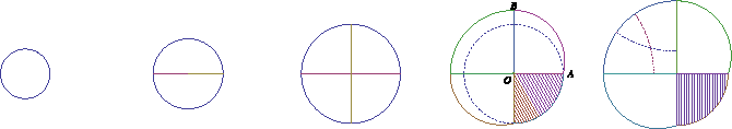
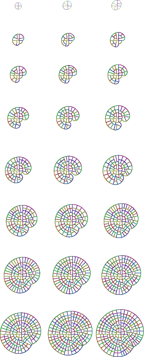
A Coleochaete cell divides into two parts when its volume (area in two-dimension) arrives at a fixed value. The cell begins with a disc to grow, then becomes two half-discs, and then four quarter-discs (see Fig. 2). The division follows the principle of cell film being the shortest length. This standard expanding process has been proven theoretically (Besson and Dumais, 2011; Wang, et al. 2015).
The initial five simulative process.
The Coleochaete cell has two kinds of divisions, one is radial with its wall being a part of the diameter, and the other one is tangent its wall being a part of arc. Wang, et al. (2015) present criteria to determine if a division is radial or tangent, which is consistent with the experiment results. One can determine the division being radial or tangent by comparing the size of the center angle \documentclass{aastex}\usepackage{amsbsy}\usepackage{amsfonts}\usepackage{amssymb}\usepackage{bm}\usepackage{mathrsfs}\usepackage{pifont}\usepackage{stmaryrd}\usepackage{textcomp}\usepackage{portland, xspace}\usepackage{amsmath, amsxtra}\pagestyle{empty}\DeclareMathSizes{10}{9}{7}{6}\begin{document}
$$\vartheta$$
\end{document} of the sector cell with the critical angle \documentclass{aastex}\usepackage{amsbsy}\usepackage{amsfonts}\usepackage{amssymb}\usepackage{bm}\usepackage{mathrsfs}\usepackage{pifont}\usepackage{stmaryrd}\usepackage{textcomp}\usepackage{portland, xspace}\usepackage{amsmath, amsxtra}\pagestyle{empty}\DeclareMathSizes{10}{9}{7}{6}\begin{document}
$${ \theta^*}$$
\end{document}, satisfying
\documentclass{aastex}\usepackage{amsbsy}\usepackage{amsfonts}\usepackage{amssymb}\usepackage{bm}\usepackage{mathrsfs}\usepackage{pifont}\usepackage{stmaryrd}\usepackage{textcomp}\usepackage{portland, xspace}\usepackage{amsmath, amsxtra}\pagestyle{empty}\DeclareMathSizes{10}{9}{7}{6}\begin{document}
\begin{align*}
{ \theta ^* } = \sqrt { \frac { 2 } { { { R^2 } + { r^2 } } } } \cdot ( R - r ). \tag { 1 }
\end{align*}
\end{document}
Here, R and r are the outer radius and radius of the sector cell respectively. The center angle \documentclass{aastex}\usepackage{amsbsy}\usepackage{amsfonts}\usepackage{amssymb}\usepackage{bm}\usepackage{mathrsfs}\usepackage{pifont}\usepackage{stmaryrd}\usepackage{textcomp}\usepackage{portland, xspace}\usepackage{amsmath, amsxtra}\pagestyle{empty}\DeclareMathSizes{10}{9}{7}{6}\begin{document}
$$\vartheta = { \theta ^*}$$
\end{document} is a threshold. This means that the division may be tangent as well as radial. And the division is radial as the center angle of the sector\documentclass{aastex}\usepackage{amsbsy}\usepackage{amsfonts}\usepackage{amssymb}\usepackage{bm}\usepackage{mathrsfs}\usepackage{pifont}\usepackage{stmaryrd}\usepackage{textcomp}\usepackage{portland, xspace}\usepackage{amsmath, amsxtra}\pagestyle{empty}\DeclareMathSizes{10}{9}{7}{6}\begin{document}
$$\vartheta > { \theta^*}$$
\end{document}, otherwise it is tangent for\documentclass{aastex}\usepackage{amsbsy}\usepackage{amsfonts}\usepackage{amssymb}\usepackage{bm}\usepackage{mathrsfs}\usepackage{pifont}\usepackage{stmaryrd}\usepackage{textcomp}\usepackage{portland, xspace}\usepackage{amsmath, amsxtra}\pagestyle{empty}\DeclareMathSizes{10}{9}{7}{6}\begin{document}
$$\vartheta < { \theta^*}$$
\end{document}. In fact, the randomness also appears in the division process, for example, the arc wall in the second quadrant of the standard cell division can be convex or concave (see the right one in Fig. 2).
A cell becomes frozen when it keeps in a situation with nogrowth and nodivision. This phenomenon has occurred in some experiments. For instance, one can find in Figure 1 that the southeast part keeps frozen like a “dead” cell.
For the discussion on nonuniform division, we assume the nonuniform cell appears after the second division like the cell in the fourth quadrant of the last two pictures in Figure 2. This cell keeps its boundary fixed and does not grow up. The other cells continue to expand symmetrically and divide, for example, the experimental images in Figure 1. Then, how can the new cells grow and divide in this nonuniform situation? We suggest an expanding model as shown in Figure 2.
A basic assumption in the following is that the new planar cell keeps its boundary as short as possible. And we also suppose that the “dead” cell keeps its shape unchanged in the nonuniform division process, and the alive cells can grow continuously. We try to determine the shapes, the boundaries, and the positions of all alive cells including the division walls.
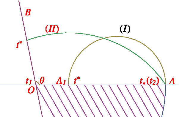
The growth model (Fig. 1) can be expressed in a mathematical problem (Fig. 3): For an angle\documentclass{aastex}\usepackage{amsbsy}\usepackage{amsfonts}\usepackage{amssymb}\usepackage{bm}\usepackage{mathrsfs}\usepackage{pifont}\usepackage{stmaryrd}\usepackage{textcomp}\usepackage{portland, xspace}\usepackage{amsmath, amsxtra}\pagestyle{empty}\DeclareMathSizes{10}{9}{7}{6}\begin{document}
$$\theta$$
\end{document}between the horizontal axis (x-axis) OA and the line OB, we need to look for a curve, like (I) or (II) inFigure 3. In this way, a planar region with fixed area is enclosed by this curve and the other two lines. It requires that one endpoint of the outer boundary should be fixed at a point A, and the other one can move on a line freely. So, how do you define the shape of curve (I) or (II) to minimize its length?
Finding the boundary with minimal length.
There's a big difference between this problem and the isoperimetric problem. The former one has two sides (lines), they form a polyline, and actually these two lines can be regarded as a curve. The third curve, the undetermined boundary, has a fixed endpoint and a free point, but the free endpoint has to comply with an undetermined boundary condition.
To find the rule that the nonstandard division process follows, we establish the objective function and constraints, then we get the Lagrangian function.
By variational method, it can be deduced that (please see the detailed demonstration in Section 6 Appendix A):
The third side, the undetermined boundary curve, is an arc and is perpendicular to the intersecting line at its free endpoint.
This result improves the theory obtained by Wang et al. (2015), meanwhile it lays the theoretical foundation for the subsequent nonstandard division.
Specifically, in Figure 3, we denote the angle between the line (another straight boundary of the cell) and the horizontal x-axis by \documentclass{aastex}\usepackage{amsbsy}\usepackage{amsfonts}\usepackage{amssymb}\usepackage{bm}\usepackage{mathrsfs}\usepackage{pifont}\usepackage{stmaryrd}\usepackage{textcomp}\usepackage{portland, xspace}\usepackage{amsmath, amsxtra}\pagestyle{empty}\DeclareMathSizes{10}{9}{7}{6}\begin{document}
$$\theta$$
\end{document}, and the union of these two lines by L. The curve (boundary to be determined) C starts from the point A on the x-axis (the parameter is \documentclass{aastex}\usepackage{amsbsy}\usepackage{amsfonts}\usepackage{amssymb}\usepackage{bm}\usepackage{mathrsfs}\usepackage{pifont}\usepackage{stmaryrd}\usepackage{textcomp}\usepackage{portland, xspace}\usepackage{amsmath, amsxtra}\pagestyle{empty}\DeclareMathSizes{10}{9}{7}{6}\begin{document}
$$t = {t_*}$$
\end{document}), the curve (I) or (II) in Figure 3, and it intersects with x-axis at point \documentclass{aastex}\usepackage{amsbsy}\usepackage{amsfonts}\usepackage{amssymb}\usepackage{bm}\usepackage{mathrsfs}\usepackage{pifont}\usepackage{stmaryrd}\usepackage{textcomp}\usepackage{portland, xspace}\usepackage{amsmath, amsxtra}\pagestyle{empty}\DeclareMathSizes{10}{9}{7}{6}\begin{document}
$${A_1} ( t = {t^*} )$$
\end{document} or with y-axis at point B1 (if it is not confusing, we still use the same parameter \documentclass{aastex}\usepackage{amsbsy}\usepackage{amsfonts}\usepackage{amssymb}\usepackage{bm}\usepackage{mathrsfs}\usepackage{pifont}\usepackage{stmaryrd}\usepackage{textcomp}\usepackage{portland, xspace}\usepackage{amsmath, amsxtra}\pagestyle{empty}\DeclareMathSizes{10}{9}{7}{6}\begin{document}
$$t = {t^*}$$
\end{document}). We write the undetermined boundary in the form of a parametric equation:
\documentclass{aastex}\usepackage{amsbsy}\usepackage{amsfonts}\usepackage{amssymb}\usepackage{bm}\usepackage{mathrsfs}\usepackage{pifont}\usepackage{stmaryrd}\usepackage{textcomp}\usepackage{portland, xspace}\usepackage{amsmath, amsxtra}\pagestyle{empty}\DeclareMathSizes{10}{9}{7}{6}\begin{document}
\begin{align*}
C: \left\{ { \begin{matrix}{x = \alpha ( t ) , } & { } \\{ y = \beta ( t ) , } & { } \\\end{matrix} } \right.t \in [ {t_ * } , {t^ * } ]. \tag{2}
\end{align*}
\end{document}
The other fixed boundary L can be expressed as the union of the following lines
\documentclass{aastex}\usepackage{amsbsy}\usepackage{amsfonts}\usepackage{amssymb}\usepackage{bm}\usepackage{mathrsfs}\usepackage{pifont}\usepackage{stmaryrd}\usepackage{textcomp}\usepackage{portland, xspace}\usepackage{amsmath, amsxtra}\pagestyle{empty}\DeclareMathSizes{10}{9}{7}{6}\begin{document}
\begin{align*}
{L_1}: \left\{ { \begin{matrix}{x = ( {t_1} - t ) \cos \theta , } & { } \\{ y = ( {t_1} - t ) \sin \theta , } & { } \\\end{matrix} } \right.t \in [ {t^ * } , {t_1} ] \ {\rm and} \ \ {L_2}: \left\{ { \begin{matrix}{x = t - {t_1} , } & { } \\ { y = 0 , }\hfill & { } \\ \end{matrix} } \right.t \in [ {t_1} , {t_2} ]. \tag{3}
\end{align*}
\end{document}
By the Lagrangian multiplier method, we can draw a variational problem of length with a condition:
\documentclass{aastex}\usepackage{amsbsy}\usepackage{amsfonts}\usepackage{amssymb}\usepackage{bm}\usepackage{mathrsfs}\usepackage{pifont}\usepackage{stmaryrd}\usepackage{textcomp}\usepackage{portland, xspace}\usepackage{amsmath, amsxtra}\pagestyle{empty}\DeclareMathSizes{10}{9}{7}{6}\begin{document}
\begin{align*}
J ( L ) = \int_ { { t_ * } } ^ { { t^ * } } \sqrt { { { ( \alpha^ { \prime } ( t ) ) } ^2 } + { { ( \beta^ { \prime } ( t ) ) } ^2 } } dt + \lambda \left( { \frac { 1 } { 2 } \oint_ { C \bigcup L } x \ dy - y \ dx - \Omega } \right). \tag { 4 }
\end{align*}
\end{document}
Here, the domain \documentclass{aastex}\usepackage{amsbsy}\usepackage{amsfonts}\usepackage{amssymb}\usepackage{bm}\usepackage{mathrsfs}\usepackage{pifont}\usepackage{stmaryrd}\usepackage{textcomp}\usepackage{portland, xspace}\usepackage{amsmath, amsxtra}\pagestyle{empty}\DeclareMathSizes{10}{9}{7}{6}\begin{document}
$$\Omega$$
\end{document} is the new cell, the enclosed area of the planar region by the fixed boundary L and the pending boundary C.
By calculation, we can see that curve C satisfies the equation
\documentclass{aastex}\usepackage{amsbsy}\usepackage{amsfonts}\usepackage{amssymb}\usepackage{bm}\usepackage{mathrsfs}\usepackage{pifont}\usepackage{stmaryrd}\usepackage{textcomp}\usepackage{portland, xspace}\usepackage{amsmath, amsxtra}\pagestyle{empty}\DeclareMathSizes{10}{9}{7}{6}\begin{document}
\begin{align*}
{ \frac { \rm { d } } { { \rm { d } } t } } \left( { { \frac { \{ \alpha^ { \prime } ( t ) , \beta^ { \prime } ( t ) \} } { \sqrt { { { ( \alpha^ { \prime } ( t ) ) } ^2 } + { { ( \beta^ { \prime } ( t ) ) } ^2 } } } } - \lambda \{ \beta ( t ) , - \alpha ( t ) \} } \right) = 0. \tag { 5 }
\end{align*}
\end{document}
Here, 0 is a zero vector on the right hand.
We can easily get the general solution of equations
\documentclass{aastex}\usepackage{amsbsy}\usepackage{amsfonts}\usepackage{amssymb}\usepackage{bm}\usepackage{mathrsfs}\usepackage{pifont}\usepackage{stmaryrd}\usepackage{textcomp}\usepackage{portland, xspace}\usepackage{amsmath, amsxtra}\pagestyle{empty}\DeclareMathSizes{10}{9}{7}{6}\begin{document}
\begin{align*}
\{ \alpha ( t ) , \beta ( t ) \} = \frac { 1 } { \lambda } \{ \sin ct , \cos ct \} + \{ { C_1 } , { C_2 } \} . \tag { 6 }
\end{align*}
\end{document}
Therefore, the curve is an arc.
By the joint conditions of the curves C and L, we can find that they are perpendicular to each other at the free intersect, that is:
\documentclass{aastex}\usepackage{amsbsy}\usepackage{amsfonts}\usepackage{amssymb}\usepackage{bm}\usepackage{mathrsfs}\usepackage{pifont}\usepackage{stmaryrd}\usepackage{textcomp}\usepackage{portland, xspace}\usepackage{amsmath, amsxtra}\pagestyle{empty}\DeclareMathSizes{10}{9}{7}{6}\begin{document}
\begin{align*}
\{ \alpha^{ \prime} ( {t^*} ) , \beta^{ \prime} ( {t^*} ) \} \cdot \{ \cos \theta , \sin \theta \} = 0. \tag{7}
\end{align*}
\end{document}
Now we can draw a conclusion that the process of cell growth and division follows rules:
The single cell begins to divide once it has grown to a fixed area (the threshold division area). For calculation purposes, in this article we set the area as 2\documentclass{aastex}\usepackage{amsbsy}\usepackage{amsfonts}\usepackage{amssymb}\usepackage{bm}\usepackage{mathrsfs}\usepackage{pifont}\usepackage{stmaryrd}\usepackage{textcomp}\usepackage{portland, xspace}\usepackage{amsmath, amsxtra}\pagestyle{empty}\DeclareMathSizes{10}{9}{7}{6}\begin{document}
$$\pi$$
\end{document}. That means the big cell will go into two individual new cells with equal area when the big one has an area of 2\documentclass{aastex}\usepackage{amsbsy}\usepackage{amsfonts}\usepackage{amssymb}\usepackage{bm}\usepackage{mathrsfs}\usepackage{pifont}\usepackage{stmaryrd}\usepackage{textcomp}\usepackage{portland, xspace}\usepackage{amsmath, amsxtra}\pagestyle{empty}\DeclareMathSizes{10}{9}{7}{6}\begin{document}
$$\pi$$
\end{document}. The division membrane of cell division follows the shortest length principle. It is theoretically based on the results of wang et al. (2015). Specifically, the division of a standard sector-shaped cell follows the criterion given byEquation (1). In the process, the interior cells won't grow or divide when they are totally surrounded, and the outer boundaries of external cells follow the shortest principle.
3. Analysis on Polyline Boundaries
As mentioned in the above section, the undetermined boundary (the outer boundary) C satisfies the conditions (5) and (7). Then, we can see from Figure 3, when the area \documentclass{aastex}\usepackage{amsbsy}\usepackage{amsfonts}\usepackage{amssymb}\usepackage{bm}\usepackage{mathrsfs}\usepackage{pifont}\usepackage{stmaryrd}\usepackage{textcomp}\usepackage{portland, xspace}\usepackage{amsmath, amsxtra}\pagestyle{empty}\DeclareMathSizes{10}{9}{7}{6}\begin{document}
$$\Omega$$
\end{document} increases, the outer boundary C, which is perpendicular to the horizontal axis, may suddenly jump to be perpendicular to another fixed boundary. It leaves us a question: When does it jump? Or what is the critical length lc of the curve C when it jumps?
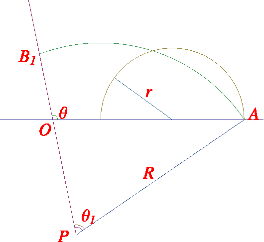
For the convenience of discussion, we assume that the length of the horizontal side OA is an unit length of 1. In Figure 4, when the length lc of C is less than the critical length lc, we denote by r the radius of the circle, and by R when lc is longer than that. The central angle corresponding to the radius R is \documentclass{aastex}\usepackage{amsbsy}\usepackage{amsfonts}\usepackage{amssymb}\usepackage{bm}\usepackage{mathrsfs}\usepackage{pifont}\usepackage{stmaryrd}\usepackage{textcomp}\usepackage{portland, xspace}\usepackage{amsmath, amsxtra}\pagestyle{empty}\DeclareMathSizes{10}{9}{7}{6}\begin{document}
$${ \theta _1}$$
\end{document}.
What is the critical length lc of the curve C when it jumps from one side to another?
Next, we will discuss the relation of the critical length lc and \documentclass{aastex}\usepackage{amsbsy}\usepackage{amsfonts}\usepackage{amssymb}\usepackage{bm}\usepackage{mathrsfs}\usepackage{pifont}\usepackage{stmaryrd}\usepackage{textcomp}\usepackage{portland, xspace}\usepackage{amsmath, amsxtra}\pagestyle{empty}\DeclareMathSizes{10}{9}{7}{6}\begin{document}
$$\theta$$
\end{document}. When the undetermined outer boundary is perpendicular to the x-axis at the free end, the length of the semicircle with its radius r is \documentclass{aastex}\usepackage{amsbsy}\usepackage{amsfonts}\usepackage{amssymb}\usepackage{bm}\usepackage{mathrsfs}\usepackage{pifont}\usepackage{stmaryrd}\usepackage{textcomp}\usepackage{portland, xspace}\usepackage{amsmath, amsxtra}\pagestyle{empty}\DeclareMathSizes{10}{9}{7}{6}\begin{document}
$$l = \pi r$$
\end{document}, and the area of the half-disk is \documentclass{aastex}\usepackage{amsbsy}\usepackage{amsfonts}\usepackage{amssymb}\usepackage{bm}\usepackage{mathrsfs}\usepackage{pifont}\usepackage{stmaryrd}\usepackage{textcomp}\usepackage{portland, xspace}\usepackage{amsmath, amsxtra}\pagestyle{empty}\DeclareMathSizes{10}{9}{7}{6}\begin{document}
$${S_r} = \pi {r^2} / 2 = {l^2} / ( 2 \pi )$$
\end{document}. When the critical length of the arc reaches and exceeds lc, the free end of the undetermined outer boundary jumps immediately to another fixed boundary. Here we can draw by sine theorem that
\documentclass{aastex}\usepackage{amsbsy}\usepackage{amsfonts}\usepackage{amssymb}\usepackage{bm}\usepackage{mathrsfs}\usepackage{pifont}\usepackage{stmaryrd}\usepackage{textcomp}\usepackage{portland, xspace}\usepackage{amsmath, amsxtra}\pagestyle{empty}\DeclareMathSizes{10}{9}{7}{6}\begin{document}
\begin{align*}
{ \theta _1 } = \arcsin \frac { { \sin ( \pi - \theta ) } } { R } .
\end{align*}
\end{document}
In this way, the cell area after the jump of the undetermined boundary can be expressed by the difference of the area of the sector APB1 with its central angle \documentclass{aastex}\usepackage{amsbsy}\usepackage{amsfonts}\usepackage{amssymb}\usepackage{bm}\usepackage{mathrsfs}\usepackage{pifont}\usepackage{stmaryrd}\usepackage{textcomp}\usepackage{portland, xspace}\usepackage{amsmath, amsxtra}\pagestyle{empty}\DeclareMathSizes{10}{9}{7}{6}\begin{document}
$${ \theta_1}$$
\end{document} and the area of the triangle \documentclass{aastex}\usepackage{amsbsy}\usepackage{amsfonts}\usepackage{amssymb}\usepackage{bm}\usepackage{mathrsfs}\usepackage{pifont}\usepackage{stmaryrd}\usepackage{textcomp}\usepackage{portland, xspace}\usepackage{amsmath, amsxtra}\pagestyle{empty}\DeclareMathSizes{10}{9}{7}{6}\begin{document}
$$\Delta APO$$
\end{document}. Note that the length of the critical arc is \documentclass{aastex}\usepackage{amsbsy}\usepackage{amsfonts}\usepackage{amssymb}\usepackage{bm}\usepackage{mathrsfs}\usepackage{pifont}\usepackage{stmaryrd}\usepackage{textcomp}\usepackage{portland, xspace}\usepackage{amsmath, amsxtra}\pagestyle{empty}\DeclareMathSizes{10}{9}{7}{6}\begin{document}
$$l = \pi r = { \theta _1}R$$
\end{document}, namely, the critical area.
\documentclass{aastex}\usepackage{amsbsy}\usepackage{amsfonts}\usepackage{amssymb}\usepackage{bm}\usepackage{mathrsfs}\usepackage{pifont}\usepackage{stmaryrd}\usepackage{textcomp}\usepackage{portland, xspace}\usepackage{amsmath, amsxtra}\pagestyle{empty}\DeclareMathSizes{10}{9}{7}{6}\begin{document}
\begin{align*}
{ \frac { { l^2 } } { 2 \pi } } = { \frac { { { ( { \theta _1 } R ) } ^2 } } { 2 \pi } } = \frac { 1 } { 2 } { R^2 } { \theta _1 } - \frac { R } { 2 } \sin ( \theta - { \theta _1 } ) \cdot 1.
\end{align*}
\end{document}
Note that, when the angle \documentclass{aastex}\usepackage{amsbsy}\usepackage{amsfonts}\usepackage{amssymb}\usepackage{bm}\usepackage{mathrsfs}\usepackage{pifont}\usepackage{stmaryrd}\usepackage{textcomp}\usepackage{portland, xspace}\usepackage{amsmath, amsxtra}\pagestyle{empty}\DeclareMathSizes{10}{9}{7}{6}\begin{document}
$$\theta$$
\end{document} is too small, this jump does not occur. Actually, when \documentclass{aastex}\usepackage{amsbsy}\usepackage{amsfonts}\usepackage{amssymb}\usepackage{bm}\usepackage{mathrsfs}\usepackage{pifont}\usepackage{stmaryrd}\usepackage{textcomp}\usepackage{portland, xspace}\usepackage{amsmath, amsxtra}\pagestyle{empty}\DeclareMathSizes{10}{9}{7}{6}\begin{document}
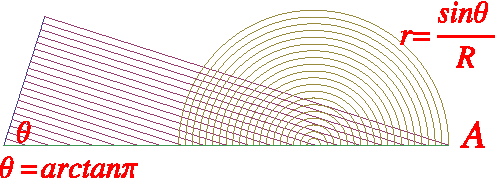
$$\theta < \arctan \pi$$
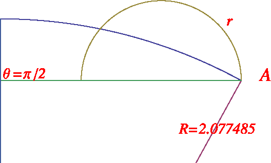
\end{document}, the shortest curve starting from the right endpoint A is a vertical line, and then this line and two boundary lines form a right triangle (see Figs. 5 and 6). We know that
\documentclass{aastex}\usepackage{amsbsy}\usepackage{amsfonts}\usepackage{amssymb}\usepackage{bm}\usepackage{mathrsfs}\usepackage{pifont}\usepackage{stmaryrd}\usepackage{textcomp}\usepackage{portland, xspace}\usepackage{amsmath, amsxtra}\pagestyle{empty}\DeclareMathSizes{10}{9}{7}{6}\begin{document}
\begin{align*}
\mathop { \lim } \limits_{ \theta \to \arctan \pi - } R = + \infty.
\end{align*}
\end{document}
The discussion on the critical length of the outer boundary: θ = arctanπ.
The discussion on the critical length of the outer boundary: θ = π/2.
Therefore, it is meaningful for discussion on the jump only when \documentclass{aastex}\usepackage{amsbsy}\usepackage{amsfonts}\usepackage{amssymb}\usepackage{bm}\usepackage{mathrsfs}\usepackage{pifont}\usepackage{stmaryrd}\usepackage{textcomp}\usepackage{portland, xspace}\usepackage{amsmath, amsxtra}\pagestyle{empty}\DeclareMathSizes{10}{9}{7}{6}\begin{document}
$$\theta$$
\end{document} is greater than \documentclass{aastex}\usepackage{amsbsy}\usepackage{amsfonts}\usepackage{amssymb}\usepackage{bm}\usepackage{mathrsfs}\usepackage{pifont}\usepackage{stmaryrd}\usepackage{textcomp}\usepackage{portland, xspace}\usepackage{amsmath, amsxtra}\pagestyle{empty}\DeclareMathSizes{10}{9}{7}{6}\begin{document}
$$\arctan \pi$$
\end{document}. Similarly, there is an upper bound for the angle \documentclass{aastex}\usepackage{amsbsy}\usepackage{amsfonts}\usepackage{amssymb}\usepackage{bm}\usepackage{mathrsfs}\usepackage{pifont}\usepackage{stmaryrd}\usepackage{textcomp}\usepackage{portland, xspace}\usepackage{amsmath, amsxtra}\pagestyle{empty}\DeclareMathSizes{10}{9}{7}{6}\begin{document}
$$\theta$$
\end{document} being 2.35 approximately. We omit detailed discussions here.
4. Division Simulation
We turn to simulate the division process by using the above rules.
In an experiment (refer to Fig. 1), a Coleochaete cell divides into two daughter cells, then four next-generation-daughter cells. The daughter cell in the fourth quadrant dies and keeps its size fixed. In Figure 2, it shows the process of growth and division from left to right. Like that, where does the right one in Figure 2 come from?
The simulated process bases theoretically of the discussion of the cell membrane growth in the article by Wang, et al. (2015), and the growth of new outer boundary (new cell membrane) comes from the theory presented in section 2. Note that in the second quadrant, cells comply with the standard division process, and we omit its discussion here (refer to Wang et al. 2015). The first and the third quadrant are symmetric, and in the following we take the cells in the first quadrant as an example to investigate.
4.1. Case 1
The cell in the first quadrant keeps its lower boundary (the upper boundary of the fourth quadrant) fixed because of the “death” of the cell in the fourth quadrant; at the same time, the former continues to grow and reaches to the area of \documentclass{aastex}\usepackage{amsbsy}\usepackage{amsfonts}\usepackage{amssymb}\usepackage{bm}\usepackage{mathrsfs}\usepackage{pifont}\usepackage{stmaryrd}\usepackage{textcomp}\usepackage{portland, xspace}\usepackage{amsmath, amsxtra}\pagestyle{empty}\DeclareMathSizes{10}{9}{7}{6}\begin{document}
$$2 \pi$$
\end{document} according to the theory in Section 2.
We can calculate and make comparisons of the length of the division arc (cell membrane, see Figure 7) specifically. When the area of the cell in the first quadrant reaches \documentclass{aastex}\usepackage{amsbsy}\usepackage{amsfonts}\usepackage{amssymb}\usepackage{bm}\usepackage{mathrsfs}\usepackage{pifont}\usepackage{stmaryrd}\usepackage{textcomp}\usepackage{portland, xspace}\usepackage{amsmath, amsxtra}\pagestyle{empty}\DeclareMathSizes{10}{9}{7}{6}\begin{document}
$$2 \pi$$
\end{document}, the center of the circle is \documentclass{aastex}\usepackage{amsbsy}\usepackage{amsfonts}\usepackage{amssymb}\usepackage{bm}\usepackage{mathrsfs}\usepackage{pifont}\usepackage{stmaryrd}\usepackage{textcomp}\usepackage{portland, xspace}\usepackage{amsmath, amsxtra}\pagestyle{empty}\DeclareMathSizes{10}{9}{7}{6}\begin{document}
$$( 0 , b ) \dot = ( 0 , 1.04815 )$$
\end{document}, and its radius is \documentclass{aastex}\usepackage{amsbsy}\usepackage{amsfonts}\usepackage{amssymb}\usepackage{bm}\usepackage{mathrsfs}\usepackage{pifont}\usepackage{stmaryrd}\usepackage{textcomp}\usepackage{portland, xspace}\usepackage{amsmath, amsxtra}\pagestyle{empty}\DeclareMathSizes{10}{9}{7}{6}\begin{document}
$$r \dot = 2.25801$$
\end{document}; the central angle with respect to this arc is \documentclass{aastex}\usepackage{amsbsy}\usepackage{amsfonts}\usepackage{amssymb}\usepackage{bm}\usepackage{mathrsfs}\usepackage{pifont}\usepackage{stmaryrd}\usepackage{textcomp}\usepackage{portland, xspace}\usepackage{amsmath, amsxtra}\pagestyle{empty}\DeclareMathSizes{10}{9}{7}{6}\begin{document}
$$\delta \dot = 2.05351$$
\end{document}. We can find that the length of the arc l1 in Figure 7 is the shortest as 2.20886. The detailed data about the radius, the center, and the length of each arc can be found in Table 1 in Appendix C.
First discussion in the first quadrant.
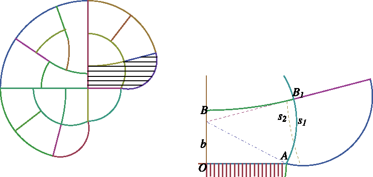
4.2. Case 2
Now we continue to discuss the division of individual parts. In the first quadrant, the outward growth of the first division arc (BB1 in Fig. 8) keeps the direction of that of the rays (tangent) of the arc BB1. And the central point of the outer boundary for new cells located on the ray, and the boundary, namely, the outer membrane, passes through point A.
Second division in the southeast corner for the first quadrant.
The boundary here being a union of three curves is different from the line boundary (y-axis), but the shape of the outer boundary is still an arc. This process can be deduced theoretically as in Appendix A. The detailed division data can be found in Table 2 in Appendix C.
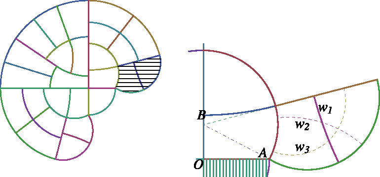
4.3. Case 3
The third division of the cell in the first quadrant begins with its central point of the outer boundary at (3.144,1.86759), and its corresponding radius is equal to 2.19012. After calculation, we find that the shortest length of the division curve of the cell is 2.16159, specifically in Figure 9 and Table 3.
Third division of the cell in the first quadrant.
4.4. Case 4
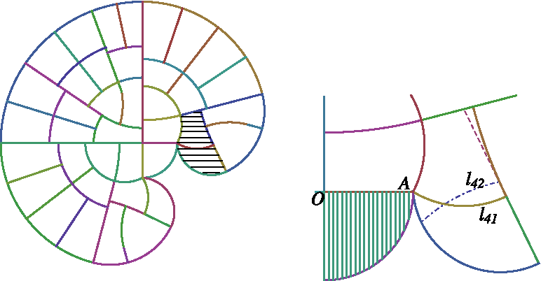
Next to case 3, the cell on the right of the division membrane w1 continuously expands in a normal way as the growth of cells in the second quadrant, and the left cell is in the constrained division. When the area of the left cell reaches \documentclass{aastex}\usepackage{amsbsy}\usepackage{amsfonts}\usepackage{amssymb}\usepackage{bm}\usepackage{mathrsfs}\usepackage{pifont}\usepackage{stmaryrd}\usepackage{textcomp}\usepackage{portland, xspace}\usepackage{amsmath, amsxtra}\pagestyle{empty}\DeclareMathSizes{10}{9}{7}{6}\begin{document}
$$2 \pi$$
\end{document}, the circle point P(3.97075, 0.160892) of the cell locates on the ray of the last cell division line, and the radius of the cell's outer membrane is 1.97731. Note that, at this moment, the outer boundary, namely the cell's outer membrane, only intersects with the boundary of the “dead” cell in the fourth quadrant at point A. In Figure 10, at this time there are two possible divisions, assumed l41, l42. By calculation, we can find that the length of division line l41 is 2.19165, and there's no solution in l42. See Table 4 for specific data.
Fourth division of the cell in the first quadrant.
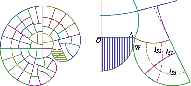
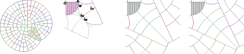
4.5. Case 5
After case 4, the division membrane l41 coincides with the membrane of the mother cell. In this way the original cell (the right cell in Fig. 10) has already been an “inner cell,” and it will not grow and divide. Only the cell on the outside will continue to grow (see Fig. 11). The detailed division data can be found in Table 5 in Appendix C.
Fifth division of the cell in the first quadrant.
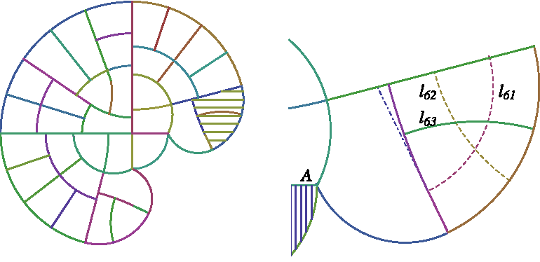
4.6. Case 6
After case 3, the cell on the right of the division membrane w1 in Figure 9 begins to grow; the left cell grows very slowly because it is pressed by its left “inner cell.” This division process is similar with case 1 (Fig. 7). The central point of the outer membrane for the lower right new cell locates at (3.144, 1.86759), and its radius is 3.06062 (Fig. 12). It can be found that the difference between this kind of division and case shows that this division membrane (\documentclass{aastex}\usepackage{amsbsy}\usepackage{amsfonts}\usepackage{amssymb}\usepackage{bm}\usepackage{mathrsfs}\usepackage{pifont}\usepackage{stmaryrd}\usepackage{textcomp}\usepackage{portland, xspace}\usepackage{amsmath, amsxtra}\pagestyle{empty}\DeclareMathSizes{10}{9}{7}{6}\begin{document}
$${l_{63}}$$
\end{document} being the shortest in Fig. 12) bends down, rather than the reverse situation in case 1. See Table 6 in Appendix C for detailed division data.
Sixth division of the cell in the first quadrant.
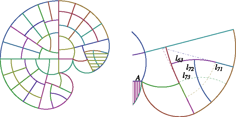
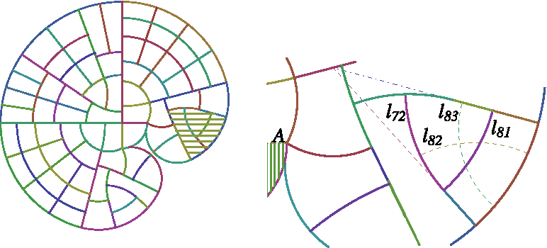
4.7. Case 7
This division is later than its left neighbor cell; its way of division is similar with case 6. There are three possible division forms when the cell grows to the threshold of the area \documentclass{aastex}\usepackage{amsbsy}\usepackage{amsfonts}\usepackage{amssymb}\usepackage{bm}\usepackage{mathrsfs}\usepackage{pifont}\usepackage{stmaryrd}\usepackage{textcomp}\usepackage{portland, xspace}\usepackage{amsmath, amsxtra}\pagestyle{empty}\DeclareMathSizes{10}{9}{7}{6}\begin{document}
$$2 \pi$$
\end{document}. After calculation, we find that the new membrane \documentclass{aastex}\usepackage{amsbsy}\usepackage{amsfonts}\usepackage{amssymb}\usepackage{bm}\usepackage{mathrsfs}\usepackage{pifont}\usepackage{stmaryrd}\usepackage{textcomp}\usepackage{portland, xspace}\usepackage{amsmath, amsxtra}\pagestyle{empty}\DeclareMathSizes{10}{9}{7}{6}\begin{document}
$${l_{72}}$$
\end{document} being 2.61411 in vertical direction is the shortest in Figure 13, and the old boundary \documentclass{aastex}\usepackage{amsbsy}\usepackage{amsfonts}\usepackage{amssymb}\usepackage{bm}\usepackage{mathrsfs}\usepackage{pifont}\usepackage{stmaryrd}\usepackage{textcomp}\usepackage{portland, xspace}\usepackage{amsmath, amsxtra}\pagestyle{empty}\DeclareMathSizes{10}{9}{7}{6}\begin{document}
$${l_{71}}$$
\end{document} of the original cell is not the shortest. The detailed division data can be found in Table 7 in Appendix C.
Seventh division of the cell in the first quadrant.
4.8. Case 8
The fast-developing group of outer cells formed in case 7 begins to divide; the central point of the outer arc still remains at (3.144, 1.86759), and its radius increases to 5.25889. It is easy to find that the division arc formed by the original outer boundary \documentclass{aastex}\usepackage{amsbsy}\usepackage{amsfonts}\usepackage{amssymb}\usepackage{bm}\usepackage{mathrsfs}\usepackage{pifont}\usepackage{stmaryrd}\usepackage{textcomp}\usepackage{portland, xspace}\usepackage{amsmath, amsxtra}\pagestyle{empty}\DeclareMathSizes{10}{9}{7}{6}\begin{document}
$${l_{81}}$$
\end{document} is the shortest one (Fig. 14 and Table 8).
Eighth division of the cell in the first quadrant.
4.9. Case 9
When the new cell formed in Case 5 is separated by \documentclass{aastex}\usepackage{amsbsy}\usepackage{amsfonts}\usepackage{amssymb}\usepackage{bm}\usepackage{mathrsfs}\usepackage{pifont}\usepackage{stmaryrd}\usepackage{textcomp}\usepackage{portland, xspace}\usepackage{amsmath, amsxtra}\pagestyle{empty}\DeclareMathSizes{10}{9}{7}{6}\begin{document}
$${l_{51}}$$
\end{document} into two daughter cells because of the cell's symmetric growth, the cells in the third quadrant will also grow accordingly, except that the outer membrane of cells will be pressed by the original “dead” cell membranes in the fourth quadrant. This leads to a common boundary in the fourth quadrant, the bisector of the fourth quadrant in Figure 15. In the expanding process, some of cells in the fourth quadrant have division arcs convex toward the center of the whole cell (refer to the right-hand pictures in Fig. 15).
Ninth division of the cell in the first quadrant.
5. Conclusion
A cell-expanding model based on the geometric shape and the area for the Coleochaete cell has been investigated in a case of nonuniform division. We mainly focus on the discussion for the expanding of the outer boundary under the assumption that a cell keeps its area frozen, that is, this cell does not change its shape. This outer boundary keeps its shape as part of a circle, and its one endpoint is fixed as well as the other one is perpendicular to a ray. The inner division curve is also an arc satisfying some conditions described by Wang et al. (2015). This model has been highly consistent with the experimental data. It presents a possibility to find the geometric mechanism for a cells' division in three dimensions.
6. Appendix A: Theoretical Analysis on Division Model
is a piecewise smooth curve, and the domain surrounded by this curve, x-axis and y-axis, is \documentclass{aastex}\usepackage{amsbsy}\usepackage{amsfonts}\usepackage{amssymb}\usepackage{bm}\usepackage{mathrsfs}\usepackage{pifont}\usepackage{stmaryrd}\usepackage{textcomp}\usepackage{portland, xspace}\usepackage{amsmath, amsxtra}\pagestyle{empty}\DeclareMathSizes{10}{9}{7}{6}\begin{document}
$$\Omega$$
\end{document}, also \documentclass{aastex}\usepackage{amsbsy}\usepackage{amsfonts}\usepackage{amssymb}\usepackage{bm}\usepackage{mathrsfs}\usepackage{pifont}\usepackage{stmaryrd}\usepackage{textcomp}\usepackage{portland, xspace}\usepackage{amsmath, amsxtra}\pagestyle{empty}\DeclareMathSizes{10}{9}{7}{6}\begin{document}
$$t = {t_*}$$
\end{document} is a fixed point; now we are looking for the shortest curve to make the area of the planar domain (we still denote it by \documentclass{aastex}\usepackage{amsbsy}\usepackage{amsfonts}\usepackage{amssymb}\usepackage{bm}\usepackage{mathrsfs}\usepackage{pifont}\usepackage{stmaryrd}\usepackage{textcomp}\usepackage{portland, xspace}\usepackage{amsmath, amsxtra}\pagestyle{empty}\DeclareMathSizes{10}{9}{7}{6}\begin{document}
$$\Omega$$
\end{document}), which is surrounded by the curve, x-axis (or probably together with y-axis) is \documentclass{aastex}\usepackage{amsbsy}\usepackage{amsfonts}\usepackage{amssymb}\usepackage{bm}\usepackage{mathrsfs}\usepackage{pifont}\usepackage{stmaryrd}\usepackage{textcomp}\usepackage{portland, xspace}\usepackage{amsmath, amsxtra}\pagestyle{empty}\DeclareMathSizes{10}{9}{7}{6}\begin{document}
$$\Omega$$
\end{document}. Another endpoint of the shortest curve is still to be determined, and we mark its parameter as \documentclass{aastex}\usepackage{amsbsy}\usepackage{amsfonts}\usepackage{amssymb}\usepackage{bm}\usepackage{mathrsfs}\usepackage{pifont}\usepackage{stmaryrd}\usepackage{textcomp}\usepackage{portland, xspace}\usepackage{amsmath, amsxtra}\pagestyle{empty}\DeclareMathSizes{10}{9}{7}{6}\begin{document}
$$t = {t^*}$$
\end{document}.
There are two situations of the pending endpoint: it can be on the x-axis or on the y-axis. We will discuss them one after another in the following.
6.1. Pending endpoint on the x-axis
In Figure 3, we denote two curves (one is a line) by
\documentclass{aastex}\usepackage{amsbsy}\usepackage{amsfonts}\usepackage{amssymb}\usepackage{bm}\usepackage{mathrsfs}\usepackage{pifont}\usepackage{stmaryrd}\usepackage{textcomp}\usepackage{portland, xspace}\usepackage{amsmath, amsxtra}\pagestyle{empty}\DeclareMathSizes{10}{9}{7}{6}\begin{document}
\begin{align*}
C: \left\{ { \begin{matrix}{x = \alpha ( t ) , } & \\ { y = \beta ( t ) , } & \\ \end{matrix} } \right.t \in [ {t_ * } , {t^ * } ]; \ \ {\rm and} \ \ L: \left\{ { \begin{matrix}{x = t - {t^ * } , } & \\ { y = 0 , }\hfill & \\ \end{matrix} } \right.t \in [ {t^ * } , {t_ * } ]. \tag{10}
\end{align*}
\end{document}
Using the Lagrangian multiplier method, we can obtain the conditional variational problem
\documentclass{aastex}\usepackage{amsbsy}\usepackage{amsfonts}\usepackage{amssymb}\usepackage{bm}\usepackage{mathrsfs}\usepackage{pifont}\usepackage{stmaryrd}\usepackage{textcomp}\usepackage{portland, xspace}\usepackage{amsmath, amsxtra}\pagestyle{empty}\DeclareMathSizes{10}{9}{7}{6}\begin{document}
\begin{align*}
J ( L ) = \int_ { { t_ * } } ^ { { t^ * } } \sqrt { { { ( \alpha^ { \prime } ( t ) ) } ^2 } + { { ( \beta^ { \prime } ( t ) ) } ^2 } } dt + \lambda \left( { \frac { 1 } { 2 } \oint_ { C \bigcup L } x { \rm { d } } y - y { \rm { d } } x - \Omega } \right). \tag { 11 }
\end{align*}
\end{document}
Therefore, the arc is vertical to the boundary at \documentclass{aastex}\usepackage{amsbsy}\usepackage{amsfonts}\usepackage{amssymb}\usepackage{bm}\usepackage{mathrsfs}\usepackage{pifont}\usepackage{stmaryrd}\usepackage{textcomp}\usepackage{portland, xspace}\usepackage{amsmath, amsxtra}\pagestyle{empty}\DeclareMathSizes{10}{9}{7}{6}\begin{document}
$$t = {t^ * }$$
\end{document}.
Let us summarize the two cases mentioned above: the shortest curve we are looking for should be an arc and is vertical to the boundary at\documentclass{aastex}\usepackage{amsbsy}\usepackage{amsfonts}\usepackage{amssymb}\usepackage{bm}\usepackage{mathrsfs}\usepackage{pifont}\usepackage{stmaryrd}\usepackage{textcomp}\usepackage{portland, xspace}\usepackage{amsmath, amsxtra}\pagestyle{empty}\DeclareMathSizes{10}{9}{7}{6}\begin{document}
$$t = {t^*}$$
\end{document}.
7. Appendix B: Table of the Status of the Division Process
We give the following diagram describing the simulating division process and a simulating video “division.avi” in the accessory (see Supplementary Video).
8. Appendix C: Table of the Data for New Cell Walls
GrahamL.E.1984. Coleochaete and the origin of land plants. Am. J. Bot., 71, 603–608.
5.
KlamkinM.S.1992. Book reviews. SIAM Rev. 34, 335–338.
6.
PrusinkiewiczS.P.2011. Inherent randomness of cell division patterns. PNAS, 108, 5933–5934.
7.
ShiB.L., and WangY.D.2012. Evolution modeling on growth image of cells. Comput. Simul., 29, 307–311 (in Chinese).
8.
SmithL.G.2001. Plant cell division: Building walls in the right places. Nat. Rev. Mol. Cell Biol., 2, 33–39.
9.
TimmeR.E., and DelwicheC.F.2010. Uncovering the evolutionary origin of plant molecular processes: Comparison of Coleochaete (Coleochaetales) and Spirogyra (Zygnematales) transcriptomes. BMC Plant Biol. 10, 96.
10.
WangY.D., DouM.Y., and ZhouZ.G.2015. The fencing problem and Coleochaete cell division. J. Math. Biol., 70, 893–912.
11.
WienerN.1914. The shortest line dividing an area in a given ratio. Proc. Camb. Philos. Soc., 18, 56–58.
Supplementary Material
Please find the following supplemental material available below.
For Open Access articles published under a Creative Commons License, all supplemental material carries the same license as the article it is associated with.
For non-Open Access articles published, all supplemental material carries a non-exclusive license, and permission requests for re-use of supplemental material or any part of supplemental material shall be sent directly to the copyright owner as specified in the copyright notice associated with the article.