A New Approach in Applying Systems Engineering Tools and Analysis to Determine Hepatocyte Toxicogenomics Risk Levels to Human Health

Abstract

There is an increasing backlog of potentially toxic compounds that cannot be evaluated with current animal-based approaches in a cost-effective and expeditious manner, thus putting human health at risk. Extrapolation of animal-based test results for human risk assessment often leads to different physiological outcomes. This article introduces the use of quantitative tools and methods from systems engineering to evaluate the risk of toxic compounds by the analysis of the amount of stress that human hepatocytes undergo in vitro when metabolizing GW7647¹ over extended times and concentrations. Hepatocytes are exceedingly connected systems that make it challenging to understand the highly varied dimensional genomics data to determine risk of exposure. Gene expression data of peroxisome proliferator-activated receptor-α (PPARα)² binding was measured over multiple concentrations and varied times of GW7647 exposure and leveraging mahalanombis distance to establish toxicity threshold risk levels. The application of these novel systems engineering tools provides new insight into the intricate workings of human hepatocytes to determine risk threshold levels from exposure. This approach is beneficial to decision makers and scientists, and it can help reduce the backlog of untested chemical compounds due to the high cost and inefficiency of animal-based models.

1. Introduction

Currently, there are more than 80,000 pre-existing, commercially available chemical compounds in use in the United States that have never been tested for toxicity risk levels. This number continues to increase by ∼2,000 per year. The European Union estimates that they need to evaluate a similar number of substances as well. When these compounds are exposed to humans, they could cause some type of human health hazard (National Research Council, 2007).

Traditional testing methods have relied on numerous laboratory animals for a single compound that is expensive and very time consuming (Bouhifd et al., 2015). Conducting a thorough risk assessment of these chemicals will require ∼54 million vertebrate animals and will cost ∼$10 billion over the next 10 years using traditional toxicity testing methods (Hartung and Rovida, 2009). There must be a revolution in toxicity testing methods to adequately evaluate each chemical in a timely manner. An alternative and new approach in applying systems engineering tools and analysis to determine toxicogenomics risk levels from hazardous compound exposure could revolutionize toxicity testing and bring it into the 21st century.

In early 2000, the Environmental Protection Agency (EPA) requested that the National Research Council (NRC) review current scientific methods to develop a new vision and strategy for toxicity testing in the 21st century. The state of science has since evolved significantly to offer alternatives to animal-based toxicity testing. New tools and methods have been at the forefront to bring in a new era of toxicity testing by leveraging systems engineering tools, systems biology tools, computational toxicology and advances in toxicogenomics, and bioinformatics. These new methods move away from animal-based models to in vitro-based methods that could evaluate human cell lines more cost effectively and efficiently.

Animal-based approaches remain very expensive when compared with in vitro methods (Humane Society International, 2007), and extrapolation of animal-based test results for human risk assessment often lead to different physiological outcomes (National Research Council, 2007). Leveraging of systems engineering tools and analysis could move the science away from slow apical-endpoint³ testing to rapid dose- and time-response testing to reduce delays. This would provide valuable information to decision makers and scientists in evaluating the potential risk of new and existing chemicals to human health in an efficient and timely manner, and therefore reduce risk (National Research Council, 2007). In 2012, the National Research Defense Council reiterated the recommendations from the NRC to strengthen toxic chemical risk assessments, especially in the areas of dose response, risk characterization, hazardous assessment, and determination of the level of exposure (Janssen et al., 2012). The systems engineering approach advocated in this article supports the extant recommendations of the NRC in toxic chemical risk assessments.

Systems engineering tools and analysis is an approach and framework that can be used to solve very complex system-of-systems problems from mechanical systems to biological systems. A system that is simple and easily understood, for example, is a desktop computer composed of numerous systems that when combined are a system-of-systems platform. The liver is composed of a system of systems, and the tools and analysis techniques from systems engineering can be applied to hepatocytes as well. A hepatocyte cell (liver cell) in a human body is composed of numerous systems and these include the lysosome, cytoplasm, nuclear membrane, vacuole, mitochondrion, ribosomes, nucleus, nucleolus, golgi, endoplasmic reticulum, centriole, peroxisome, and cell membrane. These systems make up one cell and are very complex and not completely understood. The cell interacts with numerous hepatocytes to create a network of systems that interact with other human cells. This highly complex network of systems is responsible for responding to foreign and hazardous compounds that enter the human body. Some of these compounds will be metabolized and processed by human hepatocytes. As these liver cells metabolize and process foreign compounds, the hepatocyte may recover or become highly stressed and mutate. This state of high stress can result in a malfunction in the transcription of RNA in the human liver cells during reproduction and, eventually, develop into cancer.

The overall purpose of this article is to examine the application of the systems engineering V-model to toxicity testing and to discuss how the data collection and risk evaluation process assists decision makers and scientists. This article will inform decision makers how to evaluate risk by analyzing hepatocyte multidimensional systems and unique multivariate data to make robust decisions.

By understanding the patterns of the DNA data and the underlying health risk associated with exposure of possible hazardous compounds, one can establish an appropriate risk threshold measurement system in a timely and efficient manner. The mahalanobis distance (MD) model used to evaluate risk from the collected hepatocyte data will then be explained. This article will conclude by exploring the implications of this research on current toxicity testing and areas for future research.

2. Application of Systems Engineering Tools and Analysis to Measure Toxicity in Hepatocytes

2.1. Systems engineering V-model

Systems engineering approaches have been successfully applied to human systems in reducing the incidence of methicillin-resistant staph infection (Muder et al., 2008) and in validating a pulmonary physiology simulator (Das et al., 2010). The systems engineering V-model facilitates a rapid and cost-effective approach by analyzing multi-dimensional DNA data and provides a risk threshold level to decision makers on the chemical that is being evaluated for human exposure. The systems engineering approach supports the EPA's vision of encouraging research and analysis that will lead to new risk assessment methods (U.S. Enviromental Protection Agency, 1991). The systems engineering V-model (Fig. 1) provides a framework to support the vision and strategy of toxicity testing in the 21st century.

FIG. 1.

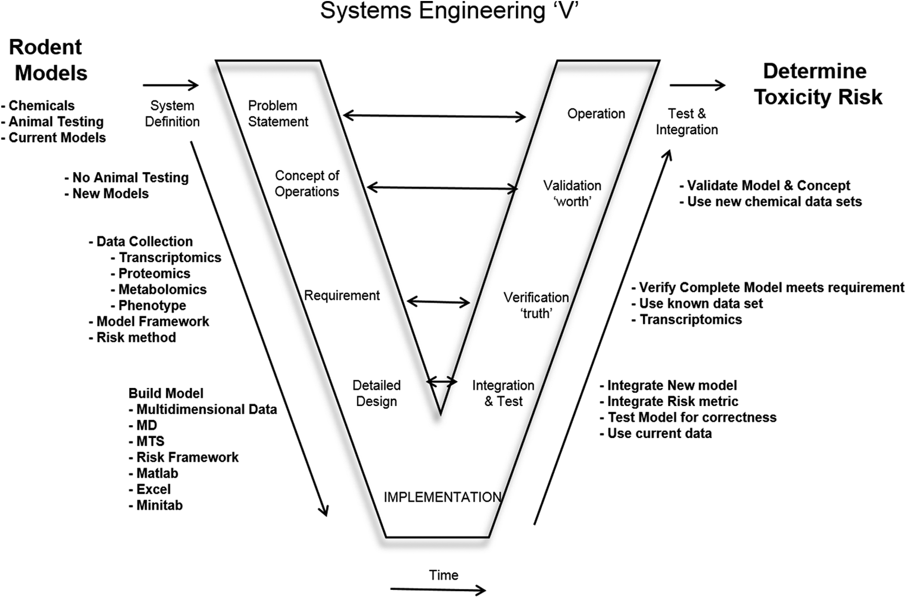
Systems Engineering V-model.

The V-model represents the sequence of steps from the problem statement to the operational solution of a systems engineering challenge. In Figure 1, the problem statement is that there are numerous chemicals that need to be tested and current rodent models and methodologies are too expensive, too time consuming, and can use a large number of animals for testing. Therefore, the concept of operation is to develop an approach that does not require rodent/animal models and is less expensive and quicker when evaluating the toxicity of chemicals.

The requirement is to collect human hepatocyte (liver cell) transcriptomics data. Transcriptomics is the study and analysis of RNA produced by the genome of the cell, a mirror image of the DNA. These data will help evaluate the effect of chemical exposure on the cells. It will help determine the amount of stress that the cells are experiencing and provide the framework for risk. Additionally, under requirements, a model framework will be established along with a risk methodology.

The detailed design will leverage MD and multidimensional DNA data from human hepatocytes along with the use of Matlab, Excel, and Minitab to evaluate the data to build a risk framework. After the implementation of the new approach through the methods previously described, integration and testing of the new approach will take place as shown by the right side of the systems engineering V-model.

Once the integration and testing phase is complete, laboratory-collected multivariate DNA data will be used to verify the approach from a known DNA response that occurs when hepatocytes are exposed to ligand⁴ GW7647. Further data will then be used to validate the response of the model in an operational setting, for example, a toxicity laboratory to determine the toxicity threshold risk from exposure of a known chemical compound.

2.2. Data collection

In Figure 1, one of the key elements in the systems engineering V-model is data collection. The Institute for Chemical Safety Science at the Hamner Institute of Health Science provided the newly collected data from recent in vitro microarray assay experiments of human hepatocytes that support this article, and all gene expression data have been made publicly available at Gene Expression Omnibus⁵—GSE53399 (McMullen et al., 2014). In general, human data are preferred to conduct a risk assessment from chemical exposure (U.S. Environmental Protection Agency, 1991). Four human donors were used to provide independent hepatocytes. These hepatocytes were exposed to GW7647 in vitro at numerous times of exposure and concentrations that resulted in 120 different experiments, of which 20 formed a baseline of unstressed cells (normal group) and 100 formed a baseline of stressed cells (abnormal group).

Microarray-based transcriptomics was used to identify statistically significant genes that were either up- or down-regulated from the 14,000 genes examined by micro-array analysis. Only 192 genes (Table 1) were identified that were of significance and exhibited a reaction to GW7647. A number of the 192 genes were analyzed using more than one probe and as a result, there were 465 different measurements or variables for each experiment. More than 80% showed up-regulation. Additionally, a majority of the 192 genes that showed up-regulation are known targets of peroxisome proliferator-activated receptor-α (PPARα) binding. PPARα are nuclear receptor proteins of the hepatocyte that regulate gene expression through transcription factors and are essential in the regulation of lipid metabolism. Thus, a majority of the up-regulated genes encompass many pathway genes that are responsible for lipid metabolism. Given next is a summary of the experiments, and Table 1 is a summary of the collected data.

Table 1.

Human Hepatocyte Genomics Data

	Observation	1	2	3	4	5	6	7	8	9	10	……	120
	Human	Hu1153	Hu1154	Hu1155	Hu1156	Hu1157	Hu1158	Hu1159	Hu1160	Hu1161	Hu1162	……	Hu1164
	Time	2	2	2	2	2	2	6	6	6	6	……	72
	Concentration	0	0.001	0.01	0.1	1	10	0	0.001	0.01	0.1	……	10
Variable	Gene symbol
1	AADAC	11.026	10.693	10.991	11.005	10.833	11.069	10.884	10.685	10.778	11.252	……	12.020
2	ABAT	7.199	7.012	6.898	7.137	7.245	7.172	7.126	6.528	7.254	6.992	……	5.760
3	ABAT	11.574	11.534	11.447	11.783	11.493	11.659	11.439	11.370	11.454	11.501	……	11.209
4	ABAT	12.195	12.299	12.148	12.317	12.436	12.276	12.162	12.237	12.252	12.158	……	11.977
5	ABCA17P	1.946	1.913	2.225	2.167	2.167	2.300	2.198	2.108	2.195	2.346	……	2.783
6	ABCD3	5.112	4.149	5.202	5.497	5.140	5.253	5.066	4.439	4.982	5.560	……	6.460
7	ABHD1	2.168	2.128	2.209	2.167	2.124	2.222	2.116	2.013	2.125	2.833	……	2.316
8	ABHD3	8.309	8.052	8.338	8.681	8.228	8.651	8.173	8.076	8.142	8.401	……	8.896
:	:	:	:	:	:	:	:	:	:	:	:	……	:
465	ZNF423	2.546	2.185	2.505	2.133	2.199	2.393	2.341	1.963	2.160	2.504	……	3.791

Hepatocyte Cells (Human Subject): Hu1153, Hu1154, Hu1156, Hu1164

Times (hours): 2, 6, 12, 24, 72

Concentration (micro-moles: μM): 0, 0.001, 0.01, 0.1, 1, 10

Number of unique genes probed (some with multiple probes): 192

Number of gene measurements (variables): 465

Total experiments (observations): 120

Baseline experiments/normal group/reference group: 20

Perturbation experiments/abnormal group: 100

2.3. Toxicity risk modeling using MD

Another critical element in the application of the systems engineering V-model approach, as depicted in Figure 1, is the development of the model. MD will be leveraged as the model that will feed into the risk evaluation of a particular compound. MD is a pattern comparison system that calculates a single measurement that describes the amount of divergence from the mean of the data by considering the correlation between the variables. It is a process of distinguishing one group from another or an abnormal group from a normal group. It has been used effectively in numerous applications that include: data classification and forecasting (Wang et al., 2004; Adebolaji, 2014), vehicle ride and braking analysis (Cudney et al., 2007, 2008; Cudney et al., 2010), semiconductor chemical vapor disposition (Jiang and Lin, 2013), health monitoring of cooling fans (Jin et al., 2012), fault diagnosis (Wang et al., 2012), centrifugal pump failure analysis (Soylemezoglu et al., 2011), bearing failures (Soylemezoglu et al., 2010), and structure health monitoring (Jin and Chendong, 2009), all of which are mechanical in design. However, it has also been used effectively in human health areas to include: analysis of blood viscosity (Yajuan et al., 2009), breast cancer detection and analysis (Taguchi and Rajesh, 2000; Cudney et al., 2007; Kestle and Cudney, 2011; Daniels et al., 2012), and liver function analysis and liver disease treatment (Taguchi et al., 2001).

In this article, there are more than 465 different variables, for example—AADAC, ABAT, ABCA17P, and ZNF423, that are evaluated using MD. This number of variables is quite large in comparison to other applications of the method described earlier that evaluated only 5 to 160 different variables. MD is extremely sensitive to inter-variable changes from the reference data, because it takes into account the variance of the multivariate data in each direction and it also takes into account the correlation between the 465 different variables or gene measurements. This allows for a more sensitive analysis in detecting any change among the different variables being measured to determine a normal or abnormal experiment from the reference/baseline data. The reference group (normal group) is referred to as the Mahalanobis space (MS), because it contains the baseline data that are in a normal state and to which other collected data will be compared. The reference data set contains the mean, standard deviation, and correlation matrix of the variables in the normal data set. Normal in this case is considered healthy hepatocyte DNA that has not been exposed to any chemical compound. The MD is calculated as follows (Taguchi and Jungulum, 2002): \documentclass{aastex}\usepackage{amsbsy}\usepackage{amsfonts}\usepackage{amssymb}\usepackage{bm}\usepackage{mathrsfs}\usepackage{pifont}\usepackage{stmaryrd}\usepackage{textcomp}\usepackage{portland, xspace}\usepackage{amsmath, amsxtra}\pagestyle{empty}\DeclareMathSizes{10}{9}{7}{6}\begin{document} \begin{align*}M{D_j} = D_j^2 = Z_{ij}^ \prime {C^{ - 1}}{Z_{ij}} \tag{1}\end{align*} \end{document} \documentclass{aastex}\usepackage{amsbsy}\usepackage{amsfonts}\usepackage{amssymb}\usepackage{bm}\usepackage{mathrsfs}\usepackage{pifont}\usepackage{stmaryrd}\usepackage{textcomp}\usepackage{portland, xspace}\usepackage{amsmath, amsxtra}\pagestyle{empty}\DeclareMathSizes{10}{9}{7}{6}\begin{document} \begin{align*} { Z_ { ij } } = { \frac { { X_ { ij } } - { m_i } } { { s_i } } } , \tag { 2 } \end{align*} \end{document}

X_ij = value of the ith characteristic (gene) of the jth observation (experiment)

m_i = mean of the ith characteristic (gene)

s_i = standard deviation of the ith characteristic (gene)

Z_ij = (z_1j, z_2j, z_3j,…, z_kj) standardized vector of the standardized values of the X_ij

Z_ij^′ = transpose of the Z_ij standardized vector

C⁻¹ = inverse of the correlation matrix

k = total number of gene measurements (465 variables).

Equation (1) uses matrix/vector algebra to determine the MD number. It is based on the data's mean and variance for each variable and the correlation matrix of all the variables. In the simplest of terms, Equation (2) standardizes the data and finds the center of mass of all the data points; whereas the correlation matrix in Equation (1) determines the shape of how the data are distributed in the MS. The shape of the MS would look like an ellipse in two-dimensional (2D) space and would describe the amount of variability in a particular direction from the center of mass as shown in Figure 2.

FIG. 2.

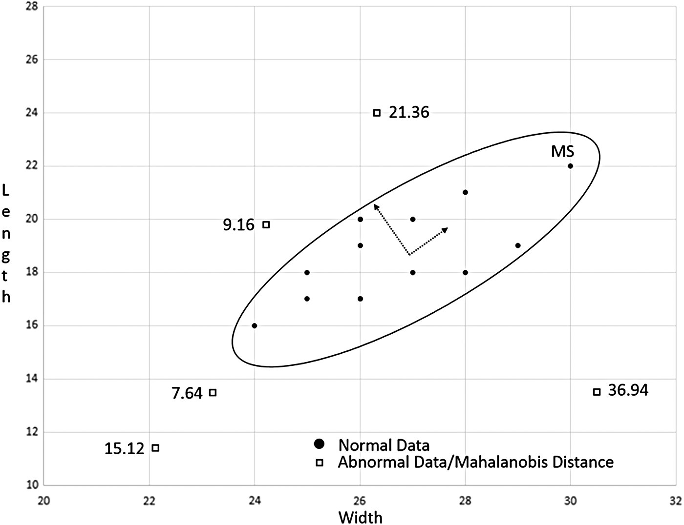
Mahalanobis space with normal and abnormal data plotted in two-dimensional space.

The MS is composed of the mean vector, standard deviation vector, and correlation matrix of the data. Once the MS is determined, Equation (1) can be used to calculate whether a randomly selected test point is within the MS. If the test point is within the MS, there is a high probability that it is a part of the group, because it is within the standard deviation from the center of mass of the normal data group. Otherwise, if it is outside the MS, it is not considered part of the group. The further away from the MS, the more significantly different the test point is from the center of mass and the normal group and the larger the calculated MD number.

It should be noted that genomics data can be highly correlated or multi-collinear across the many different variables and as a result, the correlation matrix can approach singularity. Singularity means the matrix has a determinant of zero, and the inverse correlation matrix will be undefined. As a result, the correlation matrix needs to be handled in such a manner so as to ensure that the inverse correlation matrix is neither undefined nor inaccurate. To handle this multicollinearity of the data, the inverse correlation matrix can be computed by using the adjoint matrix or by using the Moore–Penrose pseudo inverse function (Barata and Hussein, 2012). The Moore–Penrose pseudo inverse function has been widely used in data analysis applications, especially in dealing with a non-square matrix. The MD number is calculated in different stages:

(1) Stage I: Construction of the MS and measurement scale

Data must be collected to identify the reference group from the unstressed cells. These data will be used to build the MS. The MS will be determined by the normal group's mean and standard deviation vector, and the correlation matrix. The reference group will be referred to as the healthy/normal group. This is the most important aspect of the approach, as this MS will be the reference point in n-space. It is used to compare stressed hepatocyte data collected from the perturbed experiments. The measurement scale extends from the centroid of the MS and is typically one unit distance away. The centroid of the MS is the zero point for the measurement scale. The larger the MD number, the further it is from the centroid of the MS and the higher is the risk from exposure. The MD for each perturbed experiment will be derived from information describing the MS and will be shown next. The MD is a value that describes the relationship between the normal group and the experiment. As hepatocyte cells are stressed by varying concentrations and times of exposure, the same variables that were measured to establish the MS for the normal group will be used to determine an MD number for the experimental data. This MD number should be much higher than the reference group if the results of the experiment are significantly different. This MD number will be indicative of the experiment's generalized distance from the centroid of the healthy/normal group. As concentration and time of exposure increase, the MD number for that experiment could increase or decrease, depending on whether the stress of the genes is increasing or decreasing. In general, unstressed hepatocytes tend to look quite similar to the healthy/normal group, whereas stressed hepatocytes tend to look quite different from the healthy/normal group and will have a higher MD number. In addition, the changes in correlation structure among the stressed hepatocytes strongly affect the MD number. In the case where a hepatocyte's MD number reaches a predetermined high threshold value, genes may start mutating rapidly. If the MD number becomes similar to that of the healthy/normal group, the risk associated to exposure by a particular compound could be considered a low risk from exposure.

In this research, 20 different experiments were conducted to build the healthy/normal group where the cells were not exposed to GW7647. This baseline information is used to determine the amount of stress that the exposed cells are experiencing from the reference cell pattern of unstressed cells—the healthy/normal group. All the data collected in the 120 different experiments and 465 variables used the same units of measure, consistent with measuring differential gene expression data. During gene expression, the gene will produce gene products either as RNA or as proteins, and the amount of this product will be measured to determine how active the gene is. This is measured using log-base 2 to maintain symmetry and unbias between up- and down-regulated genes, and to accommodate several magnitudes of differential gene expression folding, for example, a twofold increase or decrease in gene activity. Next, the MD number for the reference experiments needs to be calculated to determine the baseline of the measurement scale that will be used to ascertain the risk threshold level.

The following is a simplistic example to show how to derive the MS and calculate the MD number for a given normal and abnormal group.

Step 1: Form a normal data set centered around (0, 0).

(a) Determine a group of normal measurements that will make up the normal group—Table 2.

(b) Calculate the mean, variance, and standard deviation for each of the column variables (width and length) as shown in Table 2.

(c) Calculate the centroid of the normal data by computing the standardized values using the appropriate mean and standard deviation for the given variable in Table 3. This causes the normal data set to be centered around (0, 0).

Table 2.

Normal Data

Normal data
Observation	Width	Length
1	24	16
2	25	18
3	26	17
4	27	18
5	28	18
6	27	20
7	29	19
8	26	20
9	28	21
10	30	22
11	25	17
12	26	17
13	26	19
14	26	20
Col_mean	26.64	18.71
Col_Var	2.709	2.989
Col_Std	1.646	1.729

Table 3.

Centroid—Standardized Matrix

	Centroid matrix Z = (x − m)/s
	1	2	3	4	5	6	7	8	9	10	11	12	13	14	Mean
Width	−1.606	−0.998	−0.391	0.217	0.825	0.217	1.432	−0.391	0.825	2.040	−0.998	−0.391	−0.391	−0.391	0
Length	−1.570	−0.413	−0.992	−0.413	−0.413	0.744	0.165	0.744	1.322	1.900	−0.992	−0.992	0.165	0.744	0

The normal data set for the hepatocyte experiments consists of the four different human liver cell lines that are exposed to 0 μM of concentration over the varying times −2, 6, 12, 24, and 72 hours from Table 1. This provides 20 observations that form the normal/reference group.

Step 2: Derive the MS in Table 4.

Table 4.

Mahalanobis Distance Space

Mahalanobis space
	Width	Length
Correlation matrix C for normal data
Width	1.000	0.691
Length	0.691	1.000
Col Mean	26.640	18.710
Col Std	1.646	1.729
Inverse correlatione matrix C⁻¹
Width	1.915	−1.324
Length	−1.324	1.915

(a) Calculate the correlation matrix of the normal data and note the mean and standard deviation of each variable from the normal data in Table 2.

(b) Calculate the inverse correlation matrix of the normal data shown in Table 4.

The normal data set of hepatocyte experiments from Table 1 will be used to derive the MS that is described by the correlation matrix, the mean vector, and the standard deviation vector as shown in this simple example.

Step 3: Derive MD for normal group.

(a) Multiply the transpose of the standardized matrix from Table 5 by the inverse correlation matrix in Table 4. This result is shown in Table 6.

(b) Multiply Table 6 by the standardized matrix in Table 3 to derive the MD for each normal data point in Table 7.

Table 5.

Centroid Transpose

Transpose Z' = (x − m)′/s
Width	Length
−1.606	−1.570
−0.998	−0.413
−0.391	−0.992
0.217	−0.413
0.825	−0.413
0.217	0.744
1.432	0.165
−0.391	0.744
0.825	1.322
2.040	1.900
−0.998	−0.992
−0.391	−0.992
−0.391	0.165
−0.391	0.744

Table 6.

Intermediate Calculations

Observation	((x − m)′/s) × C⁻¹
1	−0.997	−0.881
2	−1.365	0.530
3	0.565	−1.382
4	0.963	−1.079
5	2.126	−1.883
6	−0.569	1.137
7	2.524	−1.580
8	−1.733	1.941
9	−0.171	1.440
10	1.390	0.939
11	−0.599	−0.578
12	0.565	−1.382
13	−0.967	0.834
14	−1.733	1.941

Table 7.

Mahalanobis Distance of Normal Data

MD
2.98
1.14
1.15
0.65
2.53
0.72
3.35
2.12
1.76
4.62
1.17
1.15
0.52
2.12

MD, mahalanobis distance.

The mean of all the calculated MD values from Table 7 is 1.86. This mean value will be used as a baseline to compare against each MD number of the abnormal data. This will determine whether the test data's MD values are within the normal group or outside the normal group and by what magnitude of variability the abnormal data are different. This similar approach is used next to derive the MD number of the hepatocyte experiments for the normal data set from Table 1.

Step 4: Derive MD of experimental observations/abnormal data

(a) Analyze the experimental test data against the MS to determine whether the data are within or outside the normal group. Table 8 provides a small sample of what will be called abnormal data to demonstrate the calculations to derive the MD number for this data set. First, the abnormal data set is standardized using the mean and standard deviation from the original MS in Table 4. This will help derive the centroid matrix for the abnormal data shown in Table 9.

(b) Multiply the transpose of the standardized matrix from Table 10 by the inverse correlation matrix in Table 4. This result that is shown in Table 11 will then be multiplied by the standardized matrix in Table 9 to derive the MD number for each abnormal data point in Table 12.

Table 8.

Abnormal Data

Abnormal data
Observation	Width	Length
1	30	14
2	24	20
3	26	24
4	22	12
5	23	14

Table 9.

Centroid–Standardized Matrix

	Centroid matrix Z = (x − m)/s
	1	2	3	4	5
Width	2.040	−1.606	−0.391	−2.821	−2.213
Length	−2.727	0.744	3.057	−3.884	−2.727

Table 10.

Centroid Transpose

Transpose Z' = (x − m)′/s
Width	Length
2.040	−2.727
−1.606	0.744
−0.391	3.057
−2.821	−3.884
−2.213	−2.727

Table 11.

Intermediate Calculations

Observation	((x − m)′/s) × C⁻¹
1	7.517	−7.923
2	−4.060	3.550
3	−4.796	6.373
4	−0.261	−3.703
5	−0.629	−2.292

Table 12.

MD Abnormal Data

MD
36.94
9.16
21.36
15.12
7.64

The calculations described in step 4 for this simple example are used to derive the MD number for the varied times and concentrations (times: 2, 6, 12, 24, and 72 hours; concentrations: 0, 0.001, 0.01, 0.1, 1, and 10 μM) of the hepatocyte experiments or abnormal group from Table 1.

Step 5: Analyze experimental observations verses normal group

Determine whether the MD number for the abnormal data is within or outside the normal group or MS. Given the MD baseline of 1.86 for the normal group, it is quite resounding that the MD number for the abnormal data points (Table 12) is not within the normal group. Figure 2 depicts in 2D MS the cluster of normal data points within the solid ellipse line that represents the 1.86 MD baseline. The further the abnormal data points are from the center of the cluster, the larger the MD number indicating the amount of difference between a particular data point and the normal group. It also depicts the amount of variability in a given direction as noted by the arrows. Movement along the longer arrow's direction indicates a larger amount of variability, whereas movement along the shorter arrow's direction depicts a lesser amount of variability from the normal group. A similar analysis is performed on the hepatocyte data in Section 2.4. A 2D MS figure is not possible in the analysis for the hepatocyte data, because the MS resides in 465-dimensional space due to the large number of variables being analyzed.

(2) Stage II: Validation of measurement scale

First, conduct experiments that will stress the liver cells from exposure to GW7647, using a known agonist, and collect the data on the variables that will be used to construct the MS (Brown et al., 2001). In this article, 100 different experiments were conducted with multiple perturbations. Next, all the variables in the stressed experiments need to be normalized by using the standard deviation and mean of the healthy group. Finally, the correlation matrix from the healthy group will be used to calculate the MD space for the stressed cell experiments. If the MD scale that was developed from Stage I is acceptable, then the MD number for each of the stressed experiments should be higher than the baseline of the proposed measurement scale. Similarly, this was shown in the simple example cited earlier when comparing the abnormal data with the normal data. Figure 3 shows the flow from the selection of human liver cell lines to the establishment of the risk threshold scale that will be discussed later in the article.

FIG. 3.

Risk threshold development model.

2.4. Hepatocyte analysis

The analysis of the hepatocyte data supports the verification and validation of the systems engineering-V. MDs were computed for each of the perturbed experiments (varying time and concentration) using the correlation matrix from the healthy group. Table 13 shows the results for the human cell line 1153. The data in the table show that as the time and concentration of GW7647 increase, the MD number also increases. This response is due to additional stress that the hepatocyte system is experiencing from GW7647 exposure.

Table 13.

MD for Human 1153 Based On Different Exposure Times and Concentrations

Human	1153	1153	1153	1153	1153	1153	1153	1153	1153	1153	1153	1153	1153
Time, hours	2	2	2	2	2	6	6	6	6	6	12	12	12
Concentration, μM	0.001	0.01	0.1	1	10	0.001	0.01	0.1	1	10	0.001	0.01	0.1
MD	20.30	12.16	18.21	32.02	39.19	23.19	12.75	28.65	59.57	70.62	10.81	11.33	40.59

Human	1153	1153	1153	1153	1153	1153	1153	1153	1153	1153	1153	1153
Time, hours	12	12	24	24	24	24	24	72	72	72	72	72
Concentration, μM	1	10	0.001	0.01	0.1	1	10	0.001	0.01	0.1	1	10
MD	80.15	108.28	6.01	8.27	29.42	87.83	103.33	8.34	13.30	63.62	106.61	142.30

Additionally, the mean MDs from the four different human cell lines (1153, 1154, 1156, 1164) were computed for each of the perturbed experiments (varying time and concentration) using the correlation matrix from the healthy group, and the results are shown in Table 14. The average MD number for the four human cell lines also increases as a result of increased exposure and concentration of GW7647. Given the small sample size of 25 observations, these values support the research that Koch performed, in which he concluded that in general, biological systems typically induce a log-normal distribution (Koch, 1966), which can be seen in Figure 4.

FIG. 4.

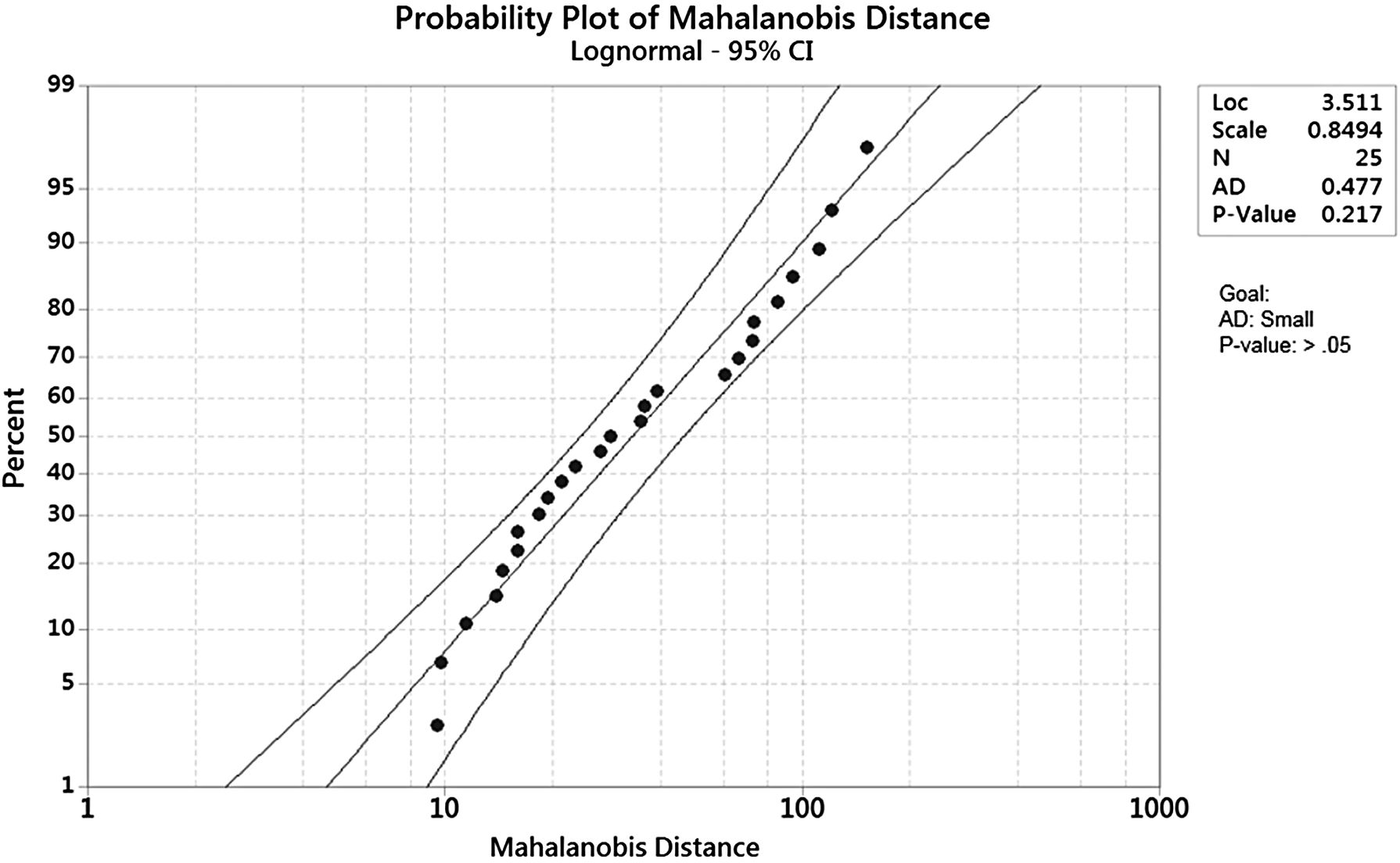
Log-normal distribution evaluation of average MD. MD, mahalanobis distance.

Table 14.

Mean MD for Humans 1153, 1154, 1156, and 1164

Time, hours	2	2	2	2	2	6	6	6	6	6	12	12	12	12	12
μM	0.001	0.01	0.1	1	10	0.001	0.01	0.1	1	10	0.001	0.01	0.1	1	10
MD mean	19.42	13.93	15.94	29.09	35.38	18.35	15.92	27.18	60.78	73.34	21.15	14.42	36.18	72.44	94.06

Time, hours	24	24	24	24	24	72	72	72	72	72
μM	0.001	0.01	0.1	1	10	0.001	0.01	0.1	1	10
MD mean	11.45	9.50	39.28	85.18	120.95	9.73	23.06	66.53	111.67	151.76

The MD results for each cell line is displayed in Figure 5 as a line plot grouped by a concentration of GW7647. The x-axis is time, and the y-axis is MD. The results for each cell line will not be identical because of the biological nature of the system. Each cell line/DNA came from a different human donor and responds differently when the cells are stressed by GW7647. However, all four cell lines have very similar graphs, and the MD number increases, in general, as the concentration and time of exposure increase. This finding shows the value and biological consistency of this approach in analyzing the change and response of the DNA from GW7647.

FIG. 5.

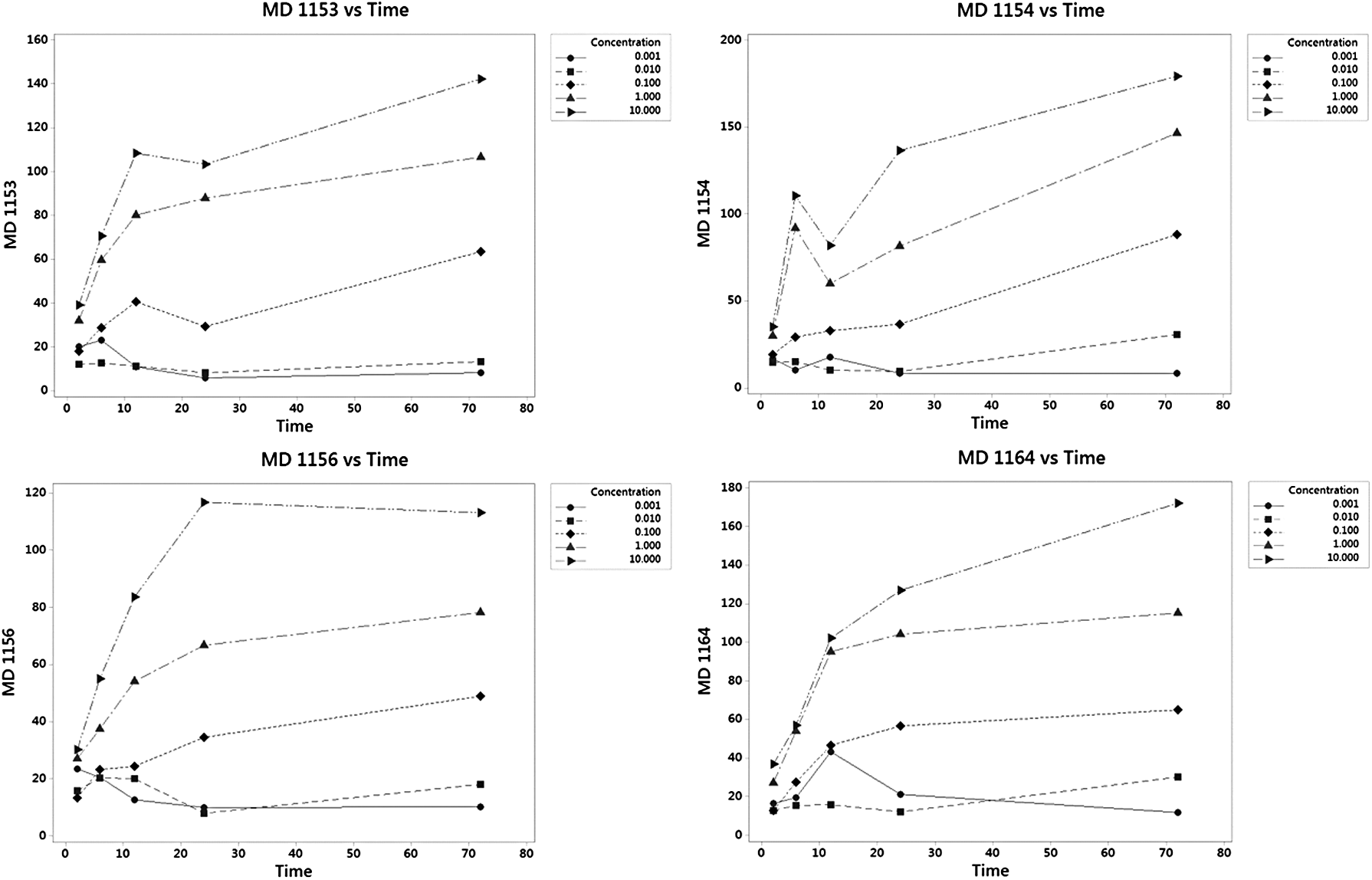
Line plot of MD by human cell line/concentration/time/MD.

Figure 6 provides further insight into the average response from the hepatocytes when exposed to GW7647 over varying times and concentrations. Once again, the MD increases, in general, as the exposure time and concentration increase. The maximum MD of 151.76 is at 72 hours with a concentration of 10.0 μM and a p-value of 0.003 at a 5% level of significance. From Figure 6, it appears that at a concentration of 0.001 and 0.01 μM, the liver cells are able to metabolize GW7647 efficiently and the amount of stress, as reflected by the MD, is starting to decrease as the length of time increases. The p-value data in Table 15 also support the fact that there is no significant difference between the healthy group and the data evaluated from 0.001 and 0.01 μM. This is not true with the other concentrations of GW7647. As concentration and time increase, the line plots clearly reflect an increased amount of stress on the genes, which accounts for a larger MD number as time and concentration levels increase. Finally, it appears as if the line plots are starting to approach the apical expression of down- or up-regulation of the genes being evaluated, for each concentration level above 0.10 μM. Additionally, in the line plots from Figures 5 and 6, the hepatocyte experiments show quite a similar response from the classical stress curve introduced by Hans Seyle for a system under stress (Selye, 1950). Figure 7 shows a modified Seyle curve for use with a biological system of cells being overly stressed and the similarities are compelling, supporting the argument that as the concentration and time of exposure increase, the hepatocytes are trying to establish a new hemeostasis state (Hartung et al., 2012).

FIG. 6.

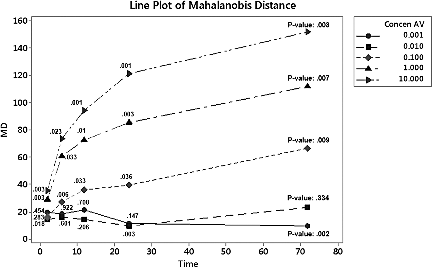
Mean MD for all human cell lines (1153, 1154, 1156, and1164) and p-values.

FIG. 7.

System under stress (Seyle, 1950; Hartung, 2012).

Table 15.

p-Values/MD at 0.05 Level of Significance

μM/h	2	6	12	24	72
0.001	0.454/19.42	0.922/18.35	0.708/21.15	0.147/11.45	0.002/9.73
0.01	0.018/13.93	0.601/15.92	0.206/14.42	0.003/9.5	0.334/23.06
0.1	0.283/15.95	0.006/27.18	0.033/36.17	0.036/39.28	0.009/66.53
1	0.003/29.09	0.033/60.78	0.01/72.44	0.003/85.18	0.007/111.67
10	0.003/35.38	0.023/73.34	0.001/94.06	0.001/120.95	0.003/151.76

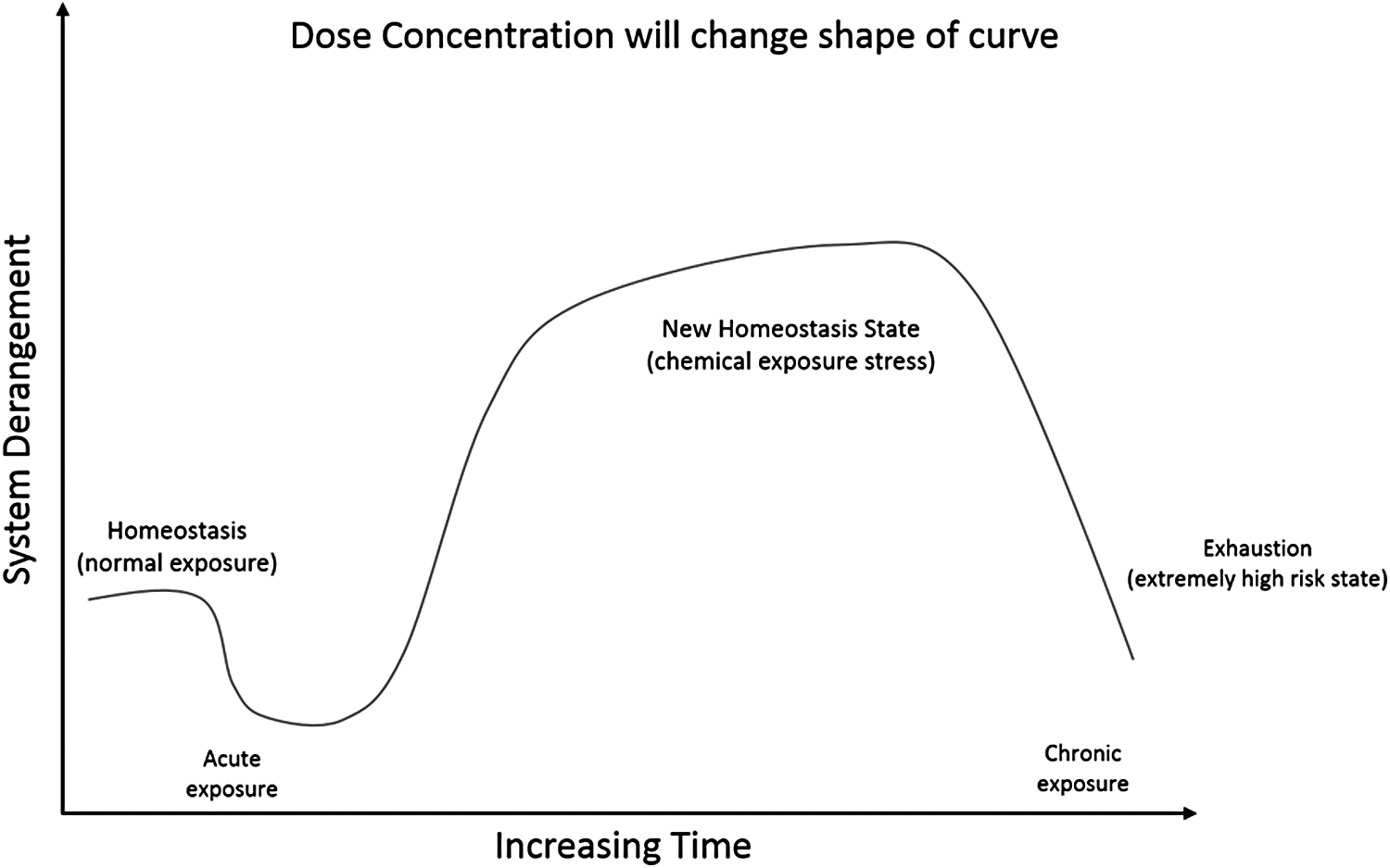
Table 15 provides a summary for the p-values for the MD number at the different times and concentration levels. Most of the MD numbers are significant, with the exceptions being the ones with p-values greater than 0.05 or less than the MD baseline of 18.05 for the healthy group. These occur mainly at concentrations levels of 0.001 and 0.01 μM. Because the insignificant values are at concentration levels of 0.001 and 0.01 μM, this implies that the cells are able to metabolize GW7647 efficiently and show no significant difference in stress than the liver cells that are not exposed to GW7647.

2.5. Toxicology threshold level

Lastly, the output of the systems engineering V-model provides a toxicity threshold level for the compound being evaluated at a given concentration level and time of exposure. Figure 8 is an approach that is used to provide a risk threshold level for GW7647 to a decision maker who is evaluating the acceptable amount of risk to human health from a particular chemical compound. The level of risk is associated with the distance from the normal/healthy group's MD baseline of 18.05. The larger the risk to human exposure, the larger the MD number from the baseline. In Figure 8, as the color of the risk threshold level gets darker, the greater is the risk to human exposure of the chemical compound being evaluated. The gradient of the risk threshold scale was calculated by the multiple deviations of the MD baseline. An MD of 36.10 would be one risk-deviation from the baseline, 54.15 would be two risk-deviations from the baseline, and 72.20 would be three risk-deviations from the baseline. Thus, the risk threshold level in Figure 8 uses an MD of 54.15, or two risk-deviations, as the maximum allowable MD to prevent risk of exposure to humans from ligand GW7647.

FIG. 8.

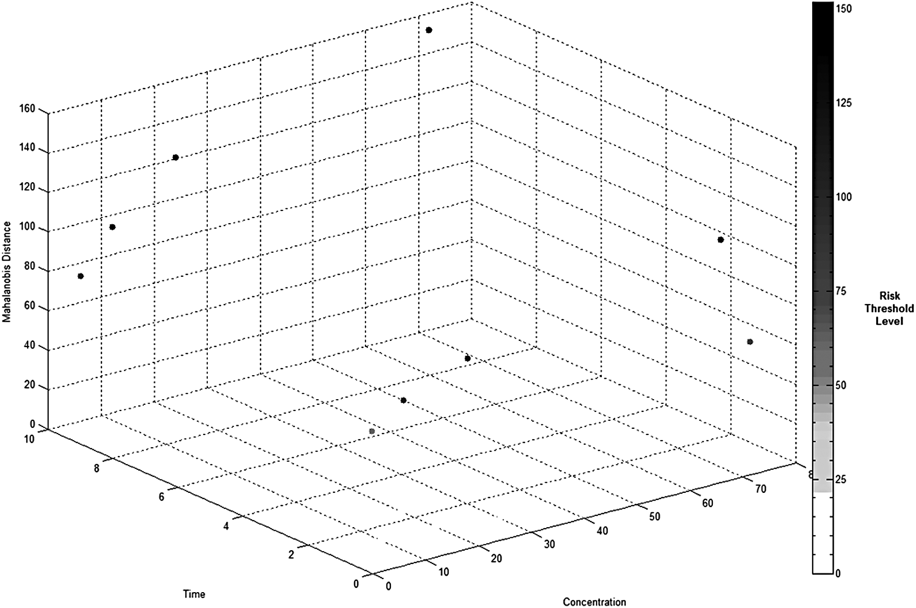
Risk threshold levels—MD versus time versus concentration.

Traditionally, existing methods rely primarily on in vivo animal testing to access toxicological risk to humans and they were designed decades ago. They are extremely time consuming and expensive to conduct at about $3 billion per year worldwide (Hartung, 2010). These decade-old methods also have low throughput rates and do not adequately predict human risk to dynamic dose-response exposure levels at the expense of millions of test animals. There is promise from this research in that it is moving away from animal testing and can be a tool to help determine initial risk of exposure. This method could work in conjunction with another non-animal-based method that compares new chemicals to the structure of known human toxic compounds (Rabesandratana, 2016). The research presented in this article is a paradigm shift from decade-old methods to a new forward-looking application of an efficient and cost-effective innovative model that does not rely on expensive animal-based methods and incorporates new emerging technologies based on human systems biology (Hartung et al., 2012).

3. Research Implications

This research suggests that dynamic dose-response models are possible when evaluating chemical compounds for risk, contrary to traditional methods using animal studies that are performed at apical doses above normal human exposure levels. Additionally, this research shows that human hepatocyte cells are a viable model when evaluating risk of exposure during initial studies for human risk. Typically, during drug development, ∼92% of drugs fail during clinical trials and 20% of those are a result of toxic side effects that were not identified during animal tests. Thus, there are concerns about the relevance and efficiency of current toxicity testing methods that use animals (Hartung, 2010). Overall, the model suggested in this research could help government and industry prescreen chemical compounds and reduce the need for expensive and lengthy animal testing by using this efficient and cost-effective approach.

4. Conclusion and Future Research

There is an escalating backlog of potentially toxic compounds that cannot be evaluated with current animal-based approaches in a cost-effective and timely manner, thus putting human health at risk. This research shows that systems engineering tools and analysis of multivariate DNA toxicogenomics data from human in vitro hepatocytes can establish toxicity threshold levels from MD calculations of potentially hazardous compounds.

Hepatocytes are complex cells with numerous subsystems, and the interactions among hepatocytes are complex and not completely understood. Gene expression patterns have been used to identify liver cancer but cannot determine the amount of risk from exposure to compounds (Chen et al., 2002). However, this systems engineering approach was shown to be an effective way to analyze the amount of stress that human hepatocytes undergo in vitro when metabolizing GW7647 over varying times and concentrations by using quantitative tools and methods that include data analysis and modeling.

Although statistical analysis is important in determining the effects of a particular compound, the biological significance of the data is the most relevant, as seen in Figure 5. The application of these tools provides new insight into the intricate workings of human hepatocytes to determine risk threshold levels from exposure. Currently, there is a paradigm shift from apical endpoints in animal testing to perturbation of toxicity pathways in human hepatocyte cells. Gene expression data of PPARα binding measured over multiple concentrations and exposure times of GW7647 doses, using MD to establish toxicity threshold risk levels, can be beneficial to decision makers and scientists, and they help reduce the backlog of untested chemical compounds due to the cost and lack of efficiency of animal-based models.

This systems engineering approach and the integration of MD strengthens toxic chemical risk assessments. It meets the need for innovation in toxicity testing as requested by the EPA, especially in the areas of dose response, risk characterization, hazardous assessment, and determining the level of exposure that is detrimental to human health. By using human hepatocytes, this approach takes into account the underlying biological response and provides a more robust estimation of the risk from exposure from a particular chemical (U.S. Environmental Protection Agency, 1991). This research has shown that new and revolutionary tools can be utilized from other engineering disciplines to help move toxicity testing into the 21st century as recommended by the NRC.

This proposed model, however, has both advantages and limitations. Its main advantage is that it supports high throughput testing and can quickly and cost effectively provide a risk determination to the potential harm to human exposure for chemical compounds without the need of lab animals. The main limitation is that it requires human hepatocyte cells in vitro for analysis and does not provide information on long-term low-level exposure accumulation and the associated risk, or the risk from compounds that are not metabolized by the liver.

Future research should be conducted to determine a suitable risk threshold level from a chemical exposure, based on the appropriate MD from the normal group's baseline. Also, additional experiments with GW7647 at longer times of exposure and concentration levels would provide the data necessary to help determine what the maximum MD number is when the genes are apically stressed or saturated and when the genes have reached stress exhaustion, as shown in Figure 7. Additionally, more work needs to be done by running similar experiments and analysis on different compounds to see whether the approach/model works as efficiently and effectively as was shown with GW7647. Finally, the application of Teguchi orthogonal arrays to the analysis of the variables that contribute significantly to the MD calculation should be explored. This research has suggested that future work in toxicity testing can accomplish the goals of reducing the number of laboratory animals used in experiments, increasing throughput, and reducing costs when attempting to determine toxicity risk to humans.

Footnotes

Acknowledgments

The Institute for Chemical Safety Science at the Hamner Institute of Health Science provided the newly collected data from recent in vitro microarray assay experiments of human hepatocytes that support this article, and all gene expression data have been made publicly available at Gene Expression Omnibus—GSE53399. There have been no financial relationships or affiliations with any commercial or government entity related to the research discussed in the article except as described earlier. Additionally, there are no other relationships or activities that have influenced the writing of this article.

Author Disclosure Statement

No competing financial interests exist.

References

Adebolaji

2014. Data classification and forecasting using the mahalanobis-taguchi method [Masters Theses]. Missouri University of Science and Technology.

Barata

J.C.

, and Hussein

M.S.

2012. The moore-penrose pseudoinvers. A tutorial review of the theory. Braz. J. Phys., 42, 146.

Bouhifd

, Andersen

M.E.

, Baghdikian

, et al. 2015. The human toxome project. ALTEX, 32, 112.

Brown

, Stuart

, Hurley

, et al. 2001. Identification of a subtype selective human PPARalpha agonist through parallel-array synthesis. Bioorg. Med. Chem. Lett., 11, 1225–7.

Chen

, Cheung

, So

, et al. 2002. Gene expression patterns in human liver cancers. Mol. Biol. Cell., 13, 1929–1939.

Cudney

, Hong

, Jugulum

, et al. 2007. An evaluation of mahalanobis-taguchi system and neural network for multivariate pattern recognition. J. Ind. Syst. Eng., 1, 139–150.

Cudney

, Paryani

, and Ragsdell

2007. Applying the mahalanobis-tagushi system to vehicle ride. J. Ind. Syst. Eng., 1, 251.

Cudney

, Paryani

, and Ragsdell

2008. Identifying useful variables for vehicle braking using the adjoint matrix approach to the mahalanobis-taguchi system. J. Ind. Syst. Eng., 1, 281–292.

Cudney

, Paryani

, and Ragsdell

2010. Forecasting consumer satisfaction for vehicle ride using the mahalanobis-taguchi gram-schmidt technique. Eng. Manage. J., 22, 3–9.

10.

Daniels

, Corns

S.M.

, and Cudney

E.A.

2012. Introduction of R-LCS and comparative analysis with FSC and mahalanobis-taguchi method for breast cancer classification. Computational Intelligence in Bioinformatics and Computational Biology (CIBCB), 2012 IEEE Symposium, San Diego, CA, pp. 283–289.

11.

Das

, Gao

, Menon

, et al. 2010. A systems engineering approach to validation of a pulmonary physiology simulator for clinical applications. J. R. Soc. Interface, 8, 44–55.

12.

Hartung

2010. Evidence-based toxicology—the toolbox of validation for the 21st century?. ALTEX 100953980, 253–263.

13.

Hartung

, and Rovida

2009. Chemical regulators have overreached. Nature, 460, 1080.

14.

Hartung

, van Vliet

E.F.

, Jaworska

J.F.

, et al. 2012. Systems toxicology. ALTEX, 29, 119.

15.

Humane Society International. 2007. Costs of animal and non-animal testing. Available at www.hsi.org/issues/chemical_product_testing/facts/time_and_cost.html (accessed Feb. 2016 )

16.

Janssen

, Sass

, Schettler

, et al. 2012. Strengthening Toxic Chemical Risk Assessments to Protect Human Health (February). National Research Defense Council. New York, NY.

17.

Jiang

, and Lin

2013. A comparison of the mahalanobis-taguchi system to A selective naive bayesian algorithm for semiconductor chemical vapor deposition process. Adv. Inf. Sci. Serv. Sci., 5, 720.

18.

Jin

, and Chendong

2009. Structural health monitoring using mahalanobis-taguchi system. Paper presented at the Information Engineering and Computer Science. 2009. ICIECS 2009. International Conference, Wuhan, pp. 1–4.

19.

Jin

, Ma

, Cheng

, et al. 2012. Health monitoring of cooling fans based on mahalanobis distance with mRMR feature selection. IEEE Trans. Instrum. Meas., 61, 2222–2229.

20.

Kestle

, and Cudney

2011. Classification application of mahalanobis-taguchi system for small datasets. Presented at Industrial Engineering Research Conference. Reno, NV.

21.

Koch

1966. The logarithm in biology. J. Theor. Biol., 23, 251.

22.

McMullen

, Bhattacharya

, Woods

, et al. 2014. A map of the PPARα transcription regulatory network for primary human hepatocytes. Chem. Biol. Interact., 209, 14–24.

23.

Muder

, Cunningham

, McCray

, et al. 2008. Implementation of an industrial systems-engineering approach to reduce the incidence of methicillin-resistant staphylococcus aureus infection. Infect. Control Hosp. Epidemiol., 20, 702–708.

24.

National Research Council. 2007. Toxicity Testing in the 21st Century: A Vision and a Strategy. The National Academies Press, Washington, DC.

25.

Rabesandratana

2016. A crystal ball for chemical safety. Science, 351, 651–651.

26.

Selye

1950. Stress and the general adaptation syndrome. Br. Med. J., 1, 1383–1392.

27.

Soylemezoglu

, Jagannathan

, and Saygin

2010. Mahalanobis taguchi system (MTS) as a prognostics tool for rolling element bearing failures. J Manuf. Sci. Eng., 132, 051014–051014.

28.

Soylemezoglu

, Jagannathan

, and Saygin

2011. Mahalanobis-taguchi system as a multi-sensor based decision making prognostics tool for centrifugal pump failures. IEEE Trans. Rel., 60, 864–878.

29.

Taguchi

, Chowdhury

, and Wu

2001. The Mahalanobis-Taguchi System. McGraw-Hill, New York, NY.

30.

Taguchi

, and Jungulum

2002. The Mahalanobis Taguchi Strategy: A Pattern Technology System. John Wiley & Sons, New York.

31.

Taguchi

, and Rajesh

2000. New trends in multivariate diagnosis. Sankhyā Ind. J. Stat. B (1960–2002), 62, 233–248.

32.

U.S. Enviromental Protection Agency. 1991. Guidelines for Developmental Toxicity Risk Assessment. (No. EPA/600/FR-91/001). Enviromental Protection Agency, Washington, DC.

33.

Wang

, Chiu

, and Su

2004. Data classification using the mahalanobis—Taguchi system. J. Chin. Inst. Ind. Eng., 21, 606–618.

34.

Wang

Zh.

, Wang

Zi.

, Tao

, and Ma

2012. Fault diagnosis for bearing based on mahalanobis-taguchi system. Paper presented at the Prognostics and System Health Management (PHM), 2012 IEEE Conference, Beijing, pp. 1–5.

35.

Yajuan

, Zhen

, and Guofang

2009. Improved mahalanobis-taguchi system and its application for potential cause analysis of abnormal observations. National Natural Science Foundation China. 12, 1–13.