Extracting Genes Involved in Disease from a Connected Network of Perturbed Biological Processes

Abstract

Metabolic disorders such as obesity and diabetes are nowadays regarded as diseases affecting majority of population. These diseases develop gradually over time in an individual. Recently, systematic experiments tracking disease progression are conducted giving a high-throughput complex data. There is a pressing need for developing methods to analyze this complex data to capture the disease mechanism at molecular level. Diseases usually develop through perturbations of biological processes in an organism. In this study, we have tried to capture the interlinking between different biological processes that work together to regulate the disease phenotype. Here, we have considered a temporal microarray data from an experiment conducted to study obesity and diabetes in mice. We have analyzed the data to obtain perturbed biological processes and developed methods to establish link between these perturbed biological processes. We have derived a mathematical formula to score genes and identified a significant set of genes regulating such a complex process network. The methods developed in our study are also applicable to a broad array of data types.

1. Introduction

Obesity and diabetes are nowadays recognized as disease affecting the majority of the population worldwide (Adams et al., 2006). On one hand, it is known that genes and proteins work together in a cell to regulate the biological functions (Barabasi and Oltvai, 2004), and perturbations of these biological functions are thought to underlie the complex physiology of a disease (Barabasi et al., 2011). Thus, understanding how different biological functions get perturbed during a disease condition could help in mechanistic understanding and further help in designing novel therapies toward such a disease (Butcher et al., 2004). On the other hand, rapid advancement in the high-throughput technologies such as microarray (Brown and Botstein, 1999; Iyer et al., 1999), RNAseq (Mortazavi et al., 2008), and proteomics (Midha et al., 2012) allows us to capture the entire cellular mechanism under disease condition through different genes and proteins (Butcher et al., 2004). These technologies are very useful in tracking and understanding progressive diseases such as obesity and diabetes.

Systematic methods have been proposed that analyze such high-throughput data to understand how different biological processes get perturbed in a disease condition. Some of these methods are clustering and biclustering. In these methods, we first find clusters of coexpressing genes and then the biological processes significantly enriched in each cluster (Eisen et al., 1998; Tamayo et al., 1999; Chen et al., 2013; Eren et al., 2013; Yosef et al., 2013). There are also other ways that include Gene Set Enrichment Analysis (Subramanian et al., 2005), which finds processes/gene lists that significantly correlate with a phenotype of interest. Gene Network Enrichment Analysis (Liu et al., 2007) finds high transcriptionally affected subnetworks in a protein–protein interaction network and looks for its significant overlap with a biological process. All these clustering and biclustering methods result in a list of significant biological processes.

In recent studies, people have started tracking disease progression over time and looking for the biological processes driving those changes. For example, Sun et al. (2013) measured gene expression from normal and diseased rats (animal model of diabetes) aged from 4 to 20 weeks, with a time interval of 4 weeks in different tissues. They identified differential expression networks and found pathways enriched in these networks both statically and temporally. Another work (He et al., 2011) looked at molecular mechanisms underlying the hepatocarcinogenesis (HCC) induced by hepatitis C virus (HCV) infection. They took the six pathologically defined disease stages in the development and progression of HCC after HCV infection. They found significant functions represented by the progression-related subnetworks that are perturbed starting from different times.

How a large number of biological processes work together temporally in a disease condition is still not known. Furthermore, it would be interesting to study the underlying genes that are regulating these processes. In this article, we aimed to capture the interdependency between different biological processes and the interconnecting genes through systems biology approaches and the network-related concepts that are used in understanding complex diseases (Barabasi et al., 2011). Furthermore, in the data analysis, we tried to incorporate the temporal dimension in identification of significant genes.

Here, we used a temporal microarray data obtained from liver of a mice fed on high-fat high-sucrose diet over an 18-week period to study obesity progression (Tikoo et al., 2013) (data present in GEO series GSE63175). Mice fed on chow diet were used as control. The high-fat diet-fed mice become obese during the mentioned period as reflected in various physiological parameters measured during the experiment.

We first focused our attention on reducing the complexity of the data by categorizing processes into a broad category of processes and studied their temporal perturbations. Then, we used the common gene concept used to make biological networks (Goh et al., 2007). Using the constructed network along with the temporal information, we identified significant genes.

2. Results

2.1. Discretizing the data and obtaining highly perturbed biological processes

The details of the experiment conducted and processing of data are given in Processing of Microarray Data section in Supplementary Material. A heat map of the microarray data given in Figure 1A shows the patterns that genes are following. We first applied the Clustered Groups (CG) algorithm (Anand and Chatterjee, 2016) on the data to get the discretized version, giving the temporal perturbations of genes. Next, we calculated the percentage perturbation (fraction of genes perturbed in at least one time point in a given process) for different biological processes. List of different biological processes along with genes present was taken from the web (see Gene Ontology Biological Process List section in Supplementary Material). We have plotted this fraction perturbation for each biological process in Figure 2B (Supplementary Fig. S3).

FIG. 1.

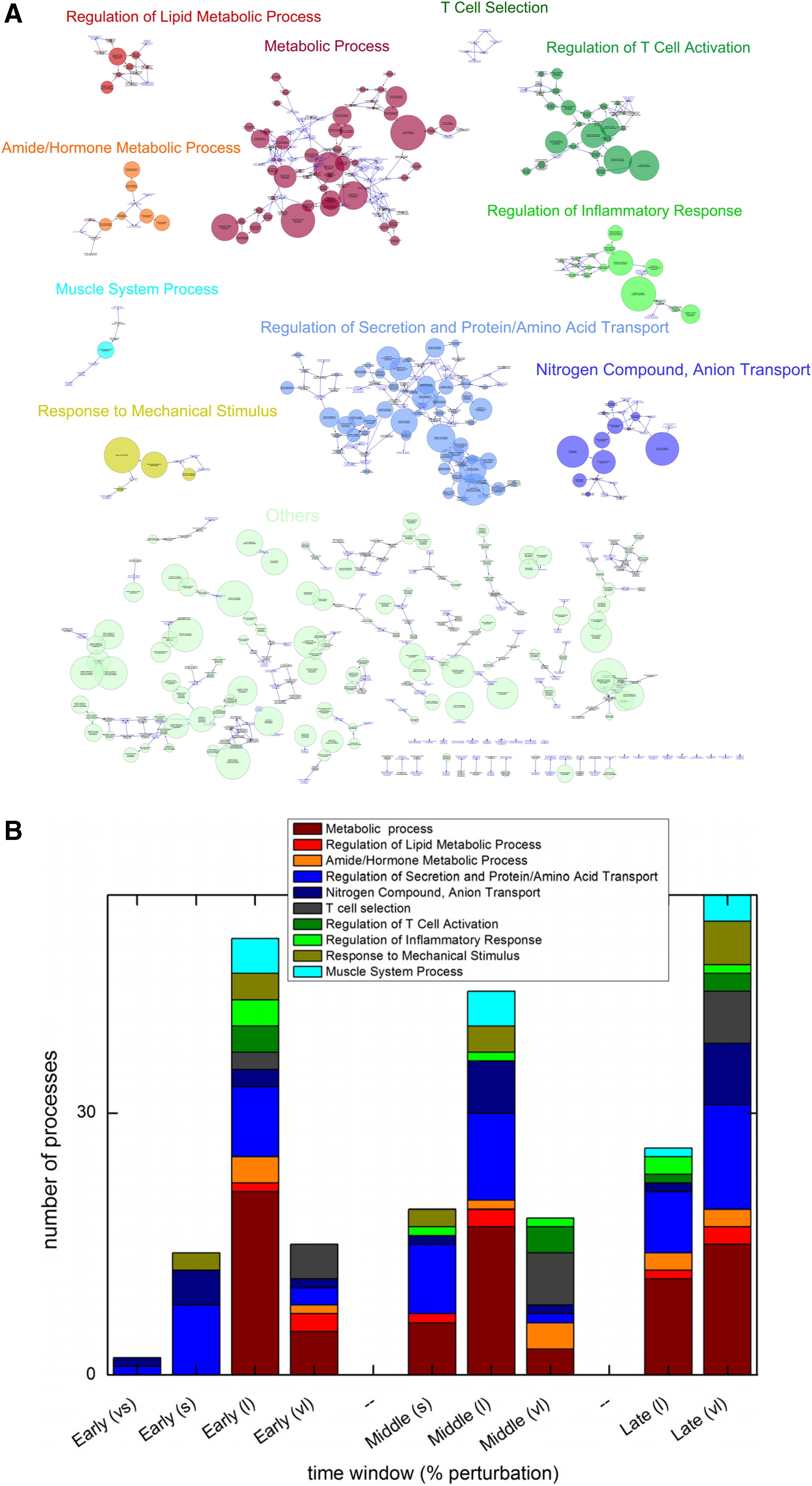
Perturbed biological processes obtained using discretizing the microarray data. (A) Heat map of the microarray data is shown with x axis as time points, y axis as genes, and color representing fold change (log₂ values). The heat map is obtained by hierarchal clustering of the original data using an algorithm by Eisen et al. (1998). (B) For each biological process (x axis), fraction of total genes perturbed is plotted in y axis and a threshold of 0.875 is used to obtain the topmost biological process (173 processes) for further analysis.

FIG. 2.

Broad categories of biological processes and their time profiles. (A) Biological process tree with perturbed biological processes and their parents are shown revealing well-separated broad category of biological processes (named and colored differently). Perturbed biological processes' node names are in blue to distinguish from other processes. (B) Figure shows the category of processes perturbed, the extent of perturbation, and the relevant time window. “Others” category is not shown in this analysis.

2.2. Grouping of list of biological processes reveals biological categories

Any database of biological processes, which are functionally close to each other, can be put together under a broad process category. The existence of functionally close biological processes is mainly because of the hierarchal-like nature of gene ontology biological process tree (Ashburner et al., 2000). A biological process database contains both the general process (parent) name and specific subprocess (child) name along with their respective genes. The genes present in a child are also present in its parent. Using different enrichment analysis tools on such a list to find significant processes would be bound to give redundant results.

To remove such redundancy and give a systematic way to separate a given list of biological processes into different broad categories, we devised a method that is based on the fact of parent–child relationship. For this, we organized the total biological processes in a tree-like form where each biological process is represented as a node and they are linked through a directed edge going from parent to child. This is a general tree and can be used in any study to categorize a list of biological processes. For example, we chose top 173 processes (with a cutoff of 0.875) for this analysis (see red dots in Fig. 1B). We built the tree by adding the parents of each of these 173 processes until we reached the general most process that has no parents as shown in Figure 2A. We found that the perturbed biological processes obtained clearly separate into different disjoint categories as shown in Figure 2A. We then selected categories that contain 3 or more perturbed processes resulting in 10 categories. We named these categories based on the general biological processes present in them, see Figure 2A. The remaining small categories are grouped under the “others” category. The perturbed biological processes present in each category are provided in Supplementary Table S1. This method helped us to reduce the redundancy that occurred during the analysis. For example, six processes linked through parent–child relationships are present in T Cell Selection category, in which one process “T Cell Selection” does not have any parent. This signifies that those five child processes are redundant and the topmost parent process can be used in place of the six processes without loss of any information.

One can use this concise information to dissect a complex data to reveal insights. For example, in our case, we wanted to dissect the temporal information hidden in the data using the biological categories. For this, we superimposed the temporal information on the biological categories to find the temporal perturbation of each category. Our data contain temporal information from 10 time points. To simplify the temporal complexity of our data, we grouped the 10 time points into different phases or windows depending on the phenotypic changes of the studied mice. According to the phenotypic data published in Midha et al. (2012), we can distinctly group the 10 time points into 3 phases based on phenotypic changes and named them as early, middle, and late phases. We calculated the fractions of total perturbed genes for each process for each phase. Next we defined four equally spaced bins on the calculated fractions to categorize each process into four degrees of perturbations. The very small perturbation (vs) falls in the bin with fraction <0.25, small perturbation(s) falls between 0.25 and 0.5, whereas the highest two perturbations (large, l, and very largest, vl) fall between 0.5 and 0.75, and >0.75, respectively. Now for each time window, we calculated the number of processes of each category that falls in different bins and plotted them as shown in Figure 2B.

Here, we found that “Regulation of Secretion and Protein/Amino Acid Transport” and “Nitrogen Compound/Anion Transport” categories of related processes follow a similar pattern: perturbed to small and large extent in early and middle phases and then perturbed to large and very large extent in late phase, see Figure 2B. The same pattern is being followed by “Muscle System” category of processes. Reasoning that processes perturbed to a very large extent, that is, >0.75 might be playing a dominant role in respective time windows, we found that “T Cell Selection”-related processes were perturbed in all three phases, but “Regulation of Inflammatory Response” and “Regulation of T Cell Activation”-related processes were mostly perturbed in middle and late phases, whereas “Metabolic Process”-related processes were perturbed largely throughout.

2.3. Connectivity between biological categories highlights important genes

The next question we want to address is whether there exists any link between processes within these categories. It might help us to understand how multiple biological processes are working together toward the development of a disease phenotype. One possibility of connecting the processes within these categories is through common genes. There are studies that have shown the importance of considering common nodes (Goh et al., 2007) and that there exists a correlation between observed simultaneous occurrences of two clusters with the fact that these are connected through common nodes (Park et al., 2009). To capture this, we constructed a network for biological processes and their linking genes (those that are common between two or more processes), see Figure 3A (Supplementary Fig. S4).

FIG. 3.

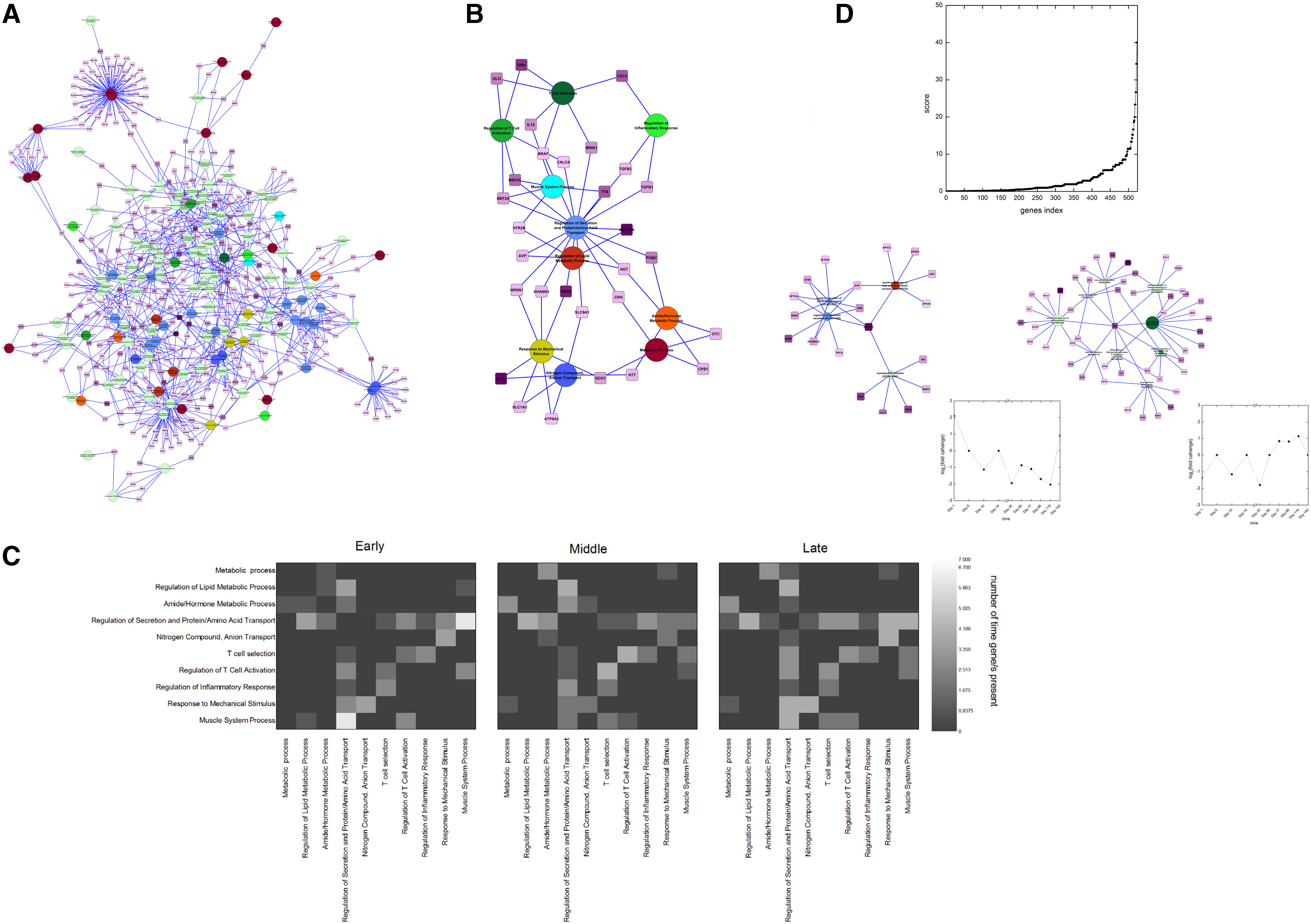
Connectivity between processes highlights important genes. (A) Depicts network between processes and genes in which a link between a gene and a process implies that the gene is present in that process. Node color of processes is same as in Figure 2A. Color gradient of genes is proportional to score of the gene (D) with dark color of gene implying high score. (B) A network between process categories and genes is shown, where a link between a gene and a process category implies the gene is present in two processes belonging to the two connecting respective categories. Color scheme of genes is the same as in (A). (C) Three heat maps are shown corresponding to early, middle, and late phases (titles). In each heat map box, the number of times the gene(s) connecting two biological process categories (shown in corresponding row and column labels) are perturbed in experiment is presented here in color: white implying large number of times and black implying less number of times. Row and column labels are same in three heat maps. (D) Sorted score (y axis) for each gene is plotted as a function of gene index (x axis). Bottom inset: two examples of genes: SHH and AVPR1A are shown ranked 1st and 13th according to our ranking (Supplementary Table S1) along with processes with which these connect to and their time profile in the data. AVPR1A, arginine vasopressin 1a receptor; SHH, sonic hedgehog.

As shown in the figure that the processes within same category are more close to each other than processes between two different categories, it may be concluded that the processes within a category are well connected. We also observed that there are some genes connecting processes from different categories and some connecting processes within the same category. Next we constructed a simplified network in which we combined biological processes from the same category as one node and linked them through connecting genes, see Figure 3B. We observed different degrees of connections in different categories. There are some highly connected categories such as “Regulation of Secretion and Protein/Amino Acid Transport,” “Regulation of Lipid Metabolic Process,” and some less connected categories such as “Regulation of Inflammatory Response” and “Regulation of T Cell Activation.”

Next, we looked for the temporal perturbation of these connecting genes. For this, we used the discretized temporal data and calculated how many times these connecting genes are perturbed at different phases, that is, early phase, in middle phase, and in late phase. This was repeated for all pairs of biological process categories and the result is depicted as heat map in Figure 3C. From the heat map we can observe that the connections between some categories change with time, whereas others do not change. For example, the category “Regulation of Secretion and Protein/Amino Acid Transport” shows high connectivity with other categories for all time points. Whereas connection between the categories “Nitrogen Compound Anion Transport” and “Amide/Hormone Metabolic Process” occurs only at the middle phase (Fig. 3C) through the connecting gene Huntingtin (HTT) (Fig. 3B).

To understand the significance of the connecting genes in our data, we obtained the correlation between the perturbations of the processes and its connecting genes (for details, see Agreement of Hypothesis with Data in Supplementary Material). We found that 84 processes out of 136 processes (∼61%) are correlating with their respective connecting genes at 6 or more time points (Supplementary Fig. S1). Thus, we may conclude that the genes connecting two processes might play a significant role in explaining the perturbation of these processes.

To test the significance of these connecting genes, we compared them with the single-nucleotide polymorphism (SNP) genes from the database of catalog of Genome Wide Association Studies (for details, see Significance of Connecting Genes Using SNP Data section in Supplementary Material). We observed that out of 25 SNP genes, 11 SNP genes are present in our list of perturbed processes, and of them 6 genes are connecting genes representing a significant 55% enrichment with p = 0.0839 (using a hypergeometric test).

So, after establishing the significance of the connecting genes, we wanted to identify which of them are more influential in terms of regulating this biological process network. For this we provided a quantitative score to all genes to reflect their influence over the entire network and then ranked them according to their scores. The proposed mathematical formula for calculating the score is based on the following assumptions:

1. High-degree nodes are more significant and influential than the low-degree nodes (Barabasi and Oltvai, 2004). Thus here we can assume that the genes connecting more processes are more influential than those connecting fewer processes. So, degree of a gene is directly proportionate to its significance.

2. We also assumed that more the number of genes present between two processes, less will be the importance of an individual gene. This is because the information flow between these processes is shared between the connecting genes, and shutting down of one or two genes will not have a significant regulation on its flow. A network measure to capture this kind of phenomena is present in network theory (Zhu et al., 2007). So, presence of more sharing genes has an inverse effect on the significance of a gene.

3. Finally, it is reasonable to assume that more the number of times a gene is perturbed, more influential it is in the disease progression. So, number of times a gene is perturbed is directly proportionate to its significance.

With these assumptions, we derived a mathematical formula for scoring a gene, say g1 and is given by \documentclass{aastex}\usepackage{amsbsy}\usepackage{amsfonts}\usepackage{amssymb}\usepackage{bm}\usepackage{mathrsfs}\usepackage{pifont}\usepackage{stmaryrd}\usepackage{textcomp}\usepackage{portland, xspace}\usepackage{amsmath, amsxtra}\usepackage{upgreek}\pagestyle{empty}\DeclareMathSizes{10}{9}{7}{6}\begin{document} \begin{align*} { \rm Score} = D \times { \rm TP} / R , \end{align*} \end{document}

where D is the biological process degree, that is, the number of biological processes connected by gene g1,

TP is number of time points, where gene g1 is perturbed, and

R is number of sharing genes, that is, the number of alternative genes present along with gene g1 between the biological processes it connects.

As the maximum values of three parameters would be different, we normalized each parameter by their respective maximum values so that they lie between 0 and 1 and then calculated the score. Using this formula, we gave score to all the 523 connecting genes present in the network of 173 processes, see Figure 3D. From the plot we can identify the most influential genes in the network by considering the top ranking genes. The list is presented in Supplementary Table S1. To establish the justification behind the selection of 173 processes, we compared the top ranked gene lists from the subnetwork of these 173 processes (small list) with the list from the whole network of 5192 processes (large list). We found that all the genes from top 10% of the small list are also in the top 10% genes of the large list. This overlap is statistically significant with a p value of <10⁻⁵. This showed that the significant genes identified from 173 processes network play an important role in influencing the entire network of 5192 processes. Hence, studying these 173 processes is enough to capture the significant information present in the network of 5192 processes.

As these genes have been obtained from liver microarray data from an experiment tracking obesity and diabetes over time, we tested the overlap of our list with a positive data set of obesity and diabetes disease genes. For this, we used the OMIM database (Hamosh et al., 2005). We calculated the precision and recall values for each cutoff (see Validation of Ranking section in Supplementary Material) and found that precision and recall were very much less (<10%) for all cutoffs when overlap between genes of our list and OMIM genes is considered. So, we find that the top genes from our list do not match much with 176 disease-specific genes from the OMIM database. So, we investigated the possibility whether the genes present in both lists are involved in same processes. For this, we calculated the precision and recall values when the processes in which genes participate in are taken into account. We plotted these precision and recall values for different cutoffs shown in Supplementary Figure S2. We saw that we reached a precision of 95% (70% average when a random list is used) when top 100 genes were used with corresponding recall value as 70% (63% average when random list is used) (i.e., capturing 123 of 176 positive genes). These top 100 genes thus correspond to ideal cutoff threshold that can be used. Thus, our ranked genes are able to capture the disease process.

3. Discussion

The idea of using common genes to connect different perturbed biological processes has already been used in a different context (Goh et al., 2007). In this study, we wanted to dissect a complex temporal microarray data obtained from mice liver tissue fed on high-fat high-sucrose diet. Here, we have used a mathematical formula (proposed and derived from network graph theory) to score genes and then ranked them to identify the most significant genes. The first step of our analysis was discretization of input data that was done using CG algorithm (Anand and Chatterjee, 2016). Here, we want to mention that one can also use any other discretization criteria such as a two-fold cutoff on gene expression values. Then, we calculated the fraction of perturbed genes for each process and then selected few top processes with high fraction of perturbed genes. We used a method to categorize such a list of perturbed processes into different categories. We ultimately used our derived mathematical formula to rank each of the connecting genes between processes in the constructed biological process network. We used a different database to validate our ranked list. The top 15 ranked genes are mentioned in Table 1 along with their respective parameters. These top ranked genes were obtained from our microarray data obtained from mice liver tissue fed on high-fat high-sucrose diet. So they should play a significant role in the development of obesity and diabetes.

Table 1.

The Top 15 Ranking Genes

Gene symbol	Gene name	Score, biological process degree, No. of sharing genes, No. of time points perturbed
SHH	Sonic Hedgehog	40, 14, 1, 6
CLN8	Ceroid-Lipofuscinosis, Neuronal 8	34.28, 9, 1, 8
PTPRC	Protein Tyrosine Phosphatase, Receptor Type, C	26.67, 7, 1, 8
DRD2	Dopamine Receptor D2	26.67, 8, 1, 7
CD74	CD74 Molecule, Major Histocompatibility Complex, Class II Invariant Chain	23.33, 7, 1, 7
CACNA1A	Calcium Channel, Voltage-Dependent, P/Q Type, Alpha 1A Subunit	23.33, 7, 1, 7
STRA6	Retinol Binding Protein 4 Receptor	20, 6, 1, 7
CCBL1	Cysteine Conjugate-Beta Lyase, Cytoplasmic	19.05, 8, 1, 5
MEF2C	Myocyte Enhancer Factor 2C	18.57, 13, 1, 3
HEY2	Hes-Related Family BHLH Transcription Factor with YRPW Motif 2	16.67, 7, 1, 5
DOCK2	Dedicator Of Cytokinesis 2	16.67, 7, 1, 5
SLITRK6	SLIT and NTRK-Like Family, Member 6	15.24, 4, 1, 8
AVPR1A	Arginine Vasopressin Receptor 1A	15.24, 4, 1, 8
LRP6	Low Density Lipoprotein Receptor-Related Protein 6	14.23, 6, 1, 5
TTN	Titin	13.33, 4, 1, 7

Available literature also validate that some of these 15 genes are influential in diabetes and obesity development. For example, sonic hedgehog (SHH) is the top ranking gene in our list. The connecting biological processes along with its temporal fold change are shown in Figure 3D bottom inset. SHH is a signal molecule essential for a variety of patterning events during development. A recent study (Swierczynska et al., 2015) has shown that diet-induced obesity in mice elevates SHH signaling in Gli1-positive progenitors. This independently supports the involvement of our top ranked gene in obesity and diabetes. Another example is the gene arginine vasopressin 1a receptor (AVPR1A), which is ranked 13th in our list. The biological processes with which the gene is connecting to along with its temporal fold change are shown in Figure 3D bottom inset. It has been shown that male AVPR1A knockout mice (V1aR^−/−) display a phenotype of low triglycerides and high glucose concentrations and high-fat diet-induced obesity and diabetes. Subjects with mutations in this gene had lower concentrations of triglycerides and a tendency toward an increased prevalence of diabetes (Enhorning et al., 2009), thus also supporting involvement of our top ranked gene in obesity and diabetes.

Our analysis provides a framework to dissect complex data to rank genes based on their importance. Our ranking captures the connectivity between perturbed processes in the data, and because the condition in our data set is time, we have also included the time dimension in our ranking. Thus, these ranked genes could play an important role in disease progression (obesity and diabetes) over time. Validation of our ranking based on positive data set of disease genes from the OMIM database confirms the accuracy by which our ranking captures the processes in which disease genes are involved. The whole methodology can also be used to analyze data from microarray, RNAseq, or proteomic experiments containing expression values in different conditions such as time as done here or in tissues.

Footnotes

Acknowledgments

The authors would like to acknowledge the contribution of Dr. K.V.S. Rao in intellectual discussions during early part of the study. This work is supported by CSIR (Government of India), grant number 25 (0258)/16/EMR-II.

Authors' Contributions

R.A. and S.C. developed the algorithm. R.A. tested the algorithm on the data and built the network. R.A. and S.C. wrote the article.

Author Disclosure Statement

No competing financial interests exist.

References

Adams

K.F.

, et al. 2006. Overweight, obesity, and mortality in a large prospective cohort of persons 50 to 71 years old. N. Engl. J. Med. 355, 763–778.

Anand

, and Chatterjee

2016. A new method of finding groups of coexpressing genes and conditions of coexpression. BMC Bioinformatics, 17, 486.

Ashburner

, et al. 2000. Gene ontology: Tool for the unification of biology. The Gene Ontology Consortium. Nat. Genet. 25, 25–29.

Barabasi

A.L.

, Gulbahce

, and Loscalzo

2011. Network medicine: A network-based approach to human disease. Nat. Rev. Genet. 12, 56–68.

Barabasi

A.L.

, and Oltvai

Z.N.

2004. Network biology: Understanding the cell's functional organization. Nat. Rev. Genet. 5, 101–113.

Brown

P.O.

, and Botstein

1999. Exploring the new world of the genome with DNA microarrays. Nat. Genet. 21, 33–37.

Butcher

E.C.

, Berg

E.L.

, and Kunkel

E.J.

2004. Systems biology in drug discovery. Nat. Biotechnol. 22, 1253–1259.

Chen

E.Y.

, et al. 2013. Enrichr: Interactive and collaborative HTML5 gene list enrichment analysis tool. BMC Bioinformatics, 14, 128.

Eisen

M.B.

, et al. 1998. Cluster analysis and display of genome-wide expression patterns. Proc. Natl. Acad. Sci. U. S. A. 95, 14863–14868.

10.

Enhorning

, et al. 2009. Relation between human vasopressin 1a gene variance, fat intake, and diabetes. Am. J. Clin. Nutr. 89, 400–406.

11.

Eren

, et al. 2013. A comparative analysis of biclustering algorithms for gene expression data. Brief Bioinform. 14, 279–292.

12.

Goh

K.I.

, et al. 2007. The human disease network. Proc. Natl. Acad. Sci. U. S. A. 104, 8685–8690.

13.

Hamosh

, et al. 2005. Online Mendelian Inheritance in Man (OMIM), a knowledgebase of human genes and genetic disorders. Nucleic Acids Res. 33, D514–D517.

14.

, Zhang

, and Shi

2011. A comprehensive analysis of the dynamic biological networks in HCV induced hepatocarcinogenesis. PLoS One, 6, e18516.

15.

Iyer

V.R.

, et al. 1999. The transcriptional program in the response of human fibroblasts to serum. Science, 283, 83–87.

16.

Liu

, et al. 2007. Network-based analysis of affected biological processes in type 2 diabetes models. PLoS Genet. 3, e96.

17.

Midha

M.K.

, et al. 2012. Extracting time-dependent obese-diabetic specific networks in hepatic proteome analysis. J. Proteome Res. 11, 6030–6043.

18.

Mortazavi

, et al. 2008. Mapping and quantifying mammalian transcriptomes by RNA-Seq. Nat. Methods, 5, 621–628.

19.

Park

, et al. 2009. The impact of cellular networks on disease comorbidity. Mol. Syst. Biol. 5, 262.

20.

Subramanian

, et al. 2005. Gene set enrichment analysis: A knowledge-based approach for interpreting genome-wide expression profiles. Proc. Natl. Acad. Sci. U. S. A. 102, 15545–15550.

21.

Sun

S.Y.

, et al. 2013. Spatio-temporal analysis of type 2 diabetes mellitus based on differential expression networks. Sci. Rep. 3, 2268.

22.

Swierczynska

M.M.

, et al. 2015. Changes in morphology and function of adrenal cortex in mice fed a high-fat diet. Int. J. Obes. (Lond.), 39, 321–330.

23.

Tamayo

, et al. 1999. Interpreting patterns of gene expression with self-organizing maps: Methods and application to hematopoietic differentiation. Proc. Natl. Acad. Sci. U. S. A., 96, 2907–2912.

24.

Tikoo

, et al. 2013. Immunomodulatory role of an ayurvedic formulation on imbalanced immunometabolics during inflammatory responses of obesity and prediabetic disease. Evid. Based Complement. Alternat. Med. 2013, 795072.

25.

Yosef

, et al. 2013. Dynamic regulatory network controlling TH17 cell differentiation. Nature, 496, 461–468.

26.

Zhu

, Gerstein

, and Snyder

2007. Getting connected: Analysis and principles of biological networks. Genes Dev. 21, 1010–1024.

Supplementary Material

Please find the following supplemental material available below.

For Open Access articles published under a Creative Commons License, all supplemental material carries the same license as the article it is associated with.

For non-Open Access articles published, all supplemental material carries a non-exclusive license, and permission requests for re-use of supplemental material or any part of supplemental material shall be sent directly to the copyright owner as specified in the copyright notice associated with the article.

0.61 MB

0.00 MB