Combinatorial Methods for Epistasis and Dominance

1.1. Linear and nonlinear models

Many models within quantitative genetics are based on the assumption of linearity or additivity, where individual alleles make additive contributions to a quantitative trait or a latent risk. Deviations from such additivity take the form of epistasis, or nonlinear interaction of contributions from multiple genes or loci, and dominance, nonlinearity within a diploid gene.

The theory of nonlinearity in quantitative genetics as developed in Sverdlov and Thompson (In Prep) distinguishes between separable traits, where a natural scale can be found on which the trait can be treated as additive, and traits possessing essential epistasis, for which no such scale exists. Consider a quantitative trait T controlled by a single diploid locus: \documentclass{aastex}\usepackage{amsbsy}\usepackage{amsfonts}\usepackage{amssymb}\usepackage{bm}\usepackage{mathrsfs}\usepackage{pifont}\usepackage{stmaryrd}\usepackage{textcomp}\usepackage{portland, xspace}\usepackage{amsmath, amsxtra}\pagestyle{empty}\DeclareMathSizes{10}{9}{7}{6}\begin{document} \begin{align*} E \left[ T \right] = \mu + { \alpha _i} + { \alpha _j} + { \delta _{ij}}. \end{align*} \end{document}

Here, the expectation is taken over possible environments, \documentclass{aastex}\usepackage{amsbsy}\usepackage{amsfonts}\usepackage{amssymb}\usepackage{bm}\usepackage{mathrsfs}\usepackage{pifont}\usepackage{stmaryrd}\usepackage{textcomp}\usepackage{portland, xspace}\usepackage{amsmath, amsxtra}\pagestyle{empty}\DeclareMathSizes{10}{9}{7}{6}\begin{document} $$\mu$$ \end{document} is an optional centering parameter and \documentclass{aastex}\usepackage{amsbsy}\usepackage{amsfonts}\usepackage{amssymb}\usepackage{bm}\usepackage{mathrsfs}\usepackage{pifont}\usepackage{stmaryrd}\usepackage{textcomp}\usepackage{portland, xspace}\usepackage{amsmath, amsxtra}\pagestyle{empty}\DeclareMathSizes{10}{9}{7}{6}\begin{document} $${ \alpha _i}$$ \end{document} is the additive effect associated with allele i. If it is possible to assign values \documentclass{aastex}\usepackage{amsbsy}\usepackage{amsfonts}\usepackage{amssymb}\usepackage{bm}\usepackage{mathrsfs}\usepackage{pifont}\usepackage{stmaryrd}\usepackage{textcomp}\usepackage{portland, xspace}\usepackage{amsmath, amsxtra}\pagestyle{empty}\DeclareMathSizes{10}{9}{7}{6}\begin{document} $${ \alpha _i}$$ \end{document} so as to make \documentclass{aastex}\usepackage{amsbsy}\usepackage{amsfonts}\usepackage{amssymb}\usepackage{bm}\usepackage{mathrsfs}\usepackage{pifont}\usepackage{stmaryrd}\usepackage{textcomp}\usepackage{portland, xspace}\usepackage{amsmath, amsxtra}\pagestyle{empty}\DeclareMathSizes{10}{9}{7}{6}\begin{document} $${ \delta _{ij}} = 0$$ \end{document} for all i and j, the trait is additive. If the trait is not additive, but there is a transformation \documentclass{aastex}\usepackage{amsbsy}\usepackage{amsfonts}\usepackage{amssymb}\usepackage{bm}\usepackage{mathrsfs}\usepackage{pifont}\usepackage{stmaryrd}\usepackage{textcomp}\usepackage{portland, xspace}\usepackage{amsmath, amsxtra}\pagestyle{empty}\DeclareMathSizes{10}{9}{7}{6}\begin{document} $$f ( \cdot )$$ \end{document} such that \documentclass{aastex}\usepackage{amsbsy}\usepackage{amsfonts}\usepackage{amssymb}\usepackage{bm}\usepackage{mathrsfs}\usepackage{pifont}\usepackage{stmaryrd}\usepackage{textcomp}\usepackage{portland, xspace}\usepackage{amsmath, amsxtra}\pagestyle{empty}\DeclareMathSizes{10}{9}{7}{6}\begin{document} \begin{align*} E \left[ {\,f ( T ) } \right] = { \mu ^{ ( f ) }} + \alpha _i^{ ( f ) } + \alpha _j^{ ( f ) } + { \delta _{ij}}, \end{align*} \end{document}

with all \documentclass{aastex}\usepackage{amsbsy}\usepackage{amsfonts}\usepackage{amssymb}\usepackage{bm}\usepackage{mathrsfs}\usepackage{pifont}\usepackage{stmaryrd}\usepackage{textcomp}\usepackage{portland, xspace}\usepackage{amsmath, amsxtra}\pagestyle{empty}\DeclareMathSizes{10}{9}{7}{6}\begin{document} $$\delta _{ij}^{ ( f ) } = 0$$ \end{document} , then the trait is separable, and the scale to which \documentclass{aastex}\usepackage{amsbsy}\usepackage{amsfonts}\usepackage{amssymb}\usepackage{bm}\usepackage{mathrsfs}\usepackage{pifont}\usepackage{stmaryrd}\usepackage{textcomp}\usepackage{portland, xspace}\usepackage{amsmath, amsxtra}\pagestyle{empty}\DeclareMathSizes{10}{9}{7}{6}\begin{document} $$f ( \cdot )$$ \end{document} transforms T is the natural scale. Additivity can be expressed in matrix notation; if we form the matrix of expected trait values \documentclass{aastex}\usepackage{amsbsy}\usepackage{amsfonts}\usepackage{amssymb}\usepackage{bm}\usepackage{mathrsfs}\usepackage{pifont}\usepackage{stmaryrd}\usepackage{textcomp}\usepackage{portland, xspace}\usepackage{amsmath, amsxtra}\pagestyle{empty}\DeclareMathSizes{10}{9}{7}{6}\begin{document} $${{ \bf{T}}_{ij}} = E \left[ {\,f \left( {{T_{ij}}} \right) } \right] = { \alpha _i} + { \alpha _j}$$ \end{document} for some vector \documentclass{aastex}\usepackage{amsbsy}\usepackage{amsfonts}\usepackage{amssymb}\usepackage{bm}\usepackage{mathrsfs}\usepackage{pifont}\usepackage{stmaryrd}\usepackage{textcomp}\usepackage{portland, xspace}\usepackage{amsmath, amsxtra}\pagestyle{empty}\DeclareMathSizes{10}{9}{7}{6}\begin{document} $$\alpha$$ \end{document} , then \documentclass{aastex}\usepackage{amsbsy}\usepackage{amsfonts}\usepackage{amssymb}\usepackage{bm}\usepackage{mathrsfs}\usepackage{pifont}\usepackage{stmaryrd}\usepackage{textcomp}\usepackage{portland, xspace}\usepackage{amsmath, amsxtra}\pagestyle{empty}\DeclareMathSizes{10}{9}{7}{6}\begin{document} \begin{align*} { \bf{T}} = \alpha^{\prime} { \bf{1}} + { \bf{1^{\prime }}} \alpha. \end{align*} \end{document}

Diploid symmetry ensures that \documentclass{aastex}\usepackage{amsbsy}\usepackage{amsfonts}\usepackage{amssymb}\usepackage{bm}\usepackage{mathrsfs}\usepackage{pifont}\usepackage{stmaryrd}\usepackage{textcomp}\usepackage{portland, xspace}\usepackage{amsmath, amsxtra}\pagestyle{empty}\DeclareMathSizes{10}{9}{7}{6}\begin{document} $${{ \bf{T}}_{ij}} = {{ \bf{T}}_{ji}}$$ \end{document} .

For the epistasis case, the phenotype in an additive model is the sum of contributions from L loci, with symmetric contributions for the paired alleles within each locus, \documentclass{aastex}\usepackage{amsbsy}\usepackage{amsfonts}\usepackage{amssymb}\usepackage{bm}\usepackage{mathrsfs}\usepackage{pifont}\usepackage{stmaryrd}\usepackage{textcomp}\usepackage{portland, xspace}\usepackage{amsmath, amsxtra}\pagestyle{empty}\DeclareMathSizes{10}{9}{7}{6}\begin{document} \begin{align*} {\rm E}\, \left[ T \right] = \mathop \sum \limits_{l = 1}^L \left( {{ \alpha _{ ( l ) i}} + { \alpha _{ ( l ) j}}} \right). \end{align*} \end{document}

As in the single locus diploid case, for a general trait T such a decomposition does not exist, but we are interested in a transformation to the natural scale \documentclass{aastex}\usepackage{amsbsy}\usepackage{amsfonts}\usepackage{amssymb}\usepackage{bm}\usepackage{mathrsfs}\usepackage{pifont}\usepackage{stmaryrd}\usepackage{textcomp}\usepackage{portland, xspace}\usepackage{amsmath, amsxtra}\pagestyle{empty}\DeclareMathSizes{10}{9}{7}{6}\begin{document} $$f ( \cdot )$$ \end{document} for which a choice of \documentclass{aastex}\usepackage{amsbsy}\usepackage{amsfonts}\usepackage{amssymb}\usepackage{bm}\usepackage{mathrsfs}\usepackage{pifont}\usepackage{stmaryrd}\usepackage{textcomp}\usepackage{portland, xspace}\usepackage{amsmath, amsxtra}\pagestyle{empty}\DeclareMathSizes{10}{9}{7}{6}\begin{document} $${ \alpha ^{ ( f ) }}$$ \end{document} exists such that \documentclass{aastex}\usepackage{amsbsy}\usepackage{amsfonts}\usepackage{amssymb}\usepackage{bm}\usepackage{mathrsfs}\usepackage{pifont}\usepackage{stmaryrd}\usepackage{textcomp}\usepackage{portland, xspace}\usepackage{amsmath, amsxtra}\pagestyle{empty}\DeclareMathSizes{10}{9}{7}{6}\begin{document} \begin{align*} {\rm E}\, \left[ {f ( T ) } \right] = \mathop \sum \limits_{l = 1}^L \left( { \alpha _{ ( l ) i}^{ ( f ) } + \alpha _{ ( l ) j}^{ ( f ) }} \right). \end{align*} \end{document}

1.2. Ordinal scale

Since we are interested in transforming traits to a natural scale, the original trait's given scale can be abstracted away. Consider the ordinal scale transformation \documentclass{aastex}\usepackage{amsbsy}\usepackage{amsfonts}\usepackage{amssymb}\usepackage{bm}\usepackage{mathrsfs}\usepackage{pifont}\usepackage{stmaryrd}\usepackage{textcomp}\usepackage{portland, xspace}\usepackage{amsmath, amsxtra}\pagestyle{empty}\DeclareMathSizes{10}{9}{7}{6}\begin{document} $$f ( {T_{ij}} ) \to rank \left( {{T_{ij}}, \left\{ {{T_{11}},{T_{12}}, \ldots {T_{nn}}} \right\} } \right)$$ \end{document} , which assigns 1 to the lowest trait value, 2 to the next higher trait value, and so on. Such a representation is as informative for the purpose of finding an original scale as the original representation. A trait architecture can be specified up to scale transformation by a complete ordering of the genotypes; an incomplete (but consistent) ordering specifies a set of trait architectures.

Our method is based on the ordering of genotypes according to their genotypic values, that is, according to the expectations of phenotypes over possible environments. A scale transformation does not always preserve order under expectation. Complications due to this phenomenon are considered in Sverdlov and Thompson (In Prep); for the purposes of computational methods developed here, we assume no environmental variability, \documentclass{aastex}\usepackage{amsbsy}\usepackage{amsfonts}\usepackage{amssymb}\usepackage{bm}\usepackage{mathrsfs}\usepackage{pifont}\usepackage{stmaryrd}\usepackage{textcomp}\usepackage{portland, xspace}\usepackage{amsmath, amsxtra}\pagestyle{empty}\DeclareMathSizes{10}{9}{7}{6}\begin{document} $${ \rm E}\ T = T$$ \end{document} and \documentclass{aastex}\usepackage{amsbsy}\usepackage{amsfonts}\usepackage{amssymb}\usepackage{bm}\usepackage{mathrsfs}\usepackage{pifont}\usepackage{stmaryrd}\usepackage{textcomp}\usepackage{portland, xspace}\usepackage{amsmath, amsxtra}\pagestyle{empty}\DeclareMathSizes{10}{9}{7}{6}\begin{document} $${ \rm E}\ f ( T ) = f ( T )$$ \end{document} , which ensures an order invariant to monotonic transformations.

1.3. Computational methods

In this article, we introduce a combinatorial approach to dominance and epistasis. Ideally, the question of whether epistasis or dominance exists as a biological phenomenon should be considered by a method invariant to monotonic transformation. This leads us to consider ordinal, rather than quantitative, traits. By specifying traits as an ordering relation or ranking over genotypes, we can ask questions about traits without reference to the scale on which they are measured. Can we choose a natural scale on which the trait is additive, that is, on which dominance and epistasis do not exist? Under what assumptions can such a scale be chosen exactly or approximately? This combinatorial approach contrasts with methods for selecting a phenotype scale by transformation to a normal phenotype distribution (e.g., Fusi et al., 2014).

We apply the combinatorial approach with similar methods to both dominance and epistasis. We demonstrate the role of directional consistency of substitution assumption and illustrate the combinatorially large number of discrete epistatic architectures, which may be classified according to biologically relevant properties.

We introduce a variety of computational tools for dealing with both separable and approximately separable traits. We develop natural scale recovery as constrained optimization problem for both the diploidy (dominance) and epistasis cases. The optimization finds an exact transformation to the natural scale if it exists and minimizes the number of ordering constraints that must be relaxed to find a solution if no exact solution exists. We develop tools to enumerate, count, or sample ordinal trait architectures satisfying certain constraints necessary but not sufficient for additivity. For the epistatic case, we develop a tool to find features within the trait architecture that explain the impossibility of finding a natural scale.

2.1. Diploid constraints and directional consistency of substitution

In the single locus, diploidy with dominance, context, we can identify several implications of additivity, which have a biological interpretation but are invariant to a monotonic transformation of the trait's scale, in particular Directional Consistency of Substitution and No Overdominance.

In Section 1.1, we described the conditions under which the trait matrix \documentclass{aastex}\usepackage{amsbsy}\usepackage{amsfonts}\usepackage{amssymb}\usepackage{bm}\usepackage{mathrsfs}\usepackage{pifont}\usepackage{stmaryrd}\usepackage{textcomp}\usepackage{portland, xspace}\usepackage{amsmath, amsxtra}\pagestyle{empty}\DeclareMathSizes{10}{9}{7}{6}\begin{document} $${{ \bf{T}}_{ij}}$$ \end{document} represents an additive trait. These conditions are implied by separability and therefore necessary for it, but not sufficient.

Consider a single diploid locus with alleles \documentclass{aastex}\usepackage{amsbsy}\usepackage{amsfonts}\usepackage{amssymb}\usepackage{bm}\usepackage{mathrsfs}\usepackage{pifont}\usepackage{stmaryrd}\usepackage{textcomp}\usepackage{portland, xspace}\usepackage{amsmath, amsxtra}\pagestyle{empty}\DeclareMathSizes{10}{9}{7}{6}\begin{document} $$A , B,C , D$$ \end{document} . We will refer to four alleles labeled by letters for convenience of exposition; the generalization to an arbitrary number of alleles is straightforward. Each pair of alleles is associated with a trait value, and we are given an ordering relation \documentclass{aastex}\usepackage{amsbsy}\usepackage{amsfonts}\usepackage{amssymb}\usepackage{bm}\usepackage{mathrsfs}\usepackage{pifont}\usepackage{stmaryrd}\usepackage{textcomp}\usepackage{portland, xspace}\usepackage{amsmath, amsxtra}\pagestyle{empty}\DeclareMathSizes{10}{9}{7}{6}\begin{document} $$\succeq$$ \end{document} on those value. It will be convenient to assume that each genotype has a unique trait value; that is, that the genotypes can be ranked with no ties, forming a complete order relation \documentclass{aastex}\usepackage{amsbsy}\usepackage{amsfonts}\usepackage{amssymb}\usepackage{bm}\usepackage{mathrsfs}\usepackage{pifont}\usepackage{stmaryrd}\usepackage{textcomp}\usepackage{portland, xspace}\usepackage{amsmath, amsxtra}\pagestyle{empty}\DeclareMathSizes{10}{9}{7}{6}\begin{document} $$\succ$$ \end{document} . We will write, for example, \documentclass{aastex}\usepackage{amsbsy}\usepackage{amsfonts}\usepackage{amssymb}\usepackage{bm}\usepackage{mathrsfs}\usepackage{pifont}\usepackage{stmaryrd}\usepackage{textcomp}\usepackage{portland, xspace}\usepackage{amsmath, amsxtra}\pagestyle{empty}\DeclareMathSizes{10}{9}{7}{6}\begin{document} $$AB \succ AC$$ \end{document} to denote that AB has trait value higher than genotype AC. Assume a complete ordering; that is, all trait values are distinct (e.g., either \documentclass{aastex}\usepackage{amsbsy}\usepackage{amsfonts}\usepackage{amssymb}\usepackage{bm}\usepackage{mathrsfs}\usepackage{pifont}\usepackage{stmaryrd}\usepackage{textcomp}\usepackage{portland, xspace}\usepackage{amsmath, amsxtra}\pagestyle{empty}\DeclareMathSizes{10}{9}{7}{6}\begin{document} $$AD \succ BC$$ \end{document} or \documentclass{aastex}\usepackage{amsbsy}\usepackage{amsfonts}\usepackage{amssymb}\usepackage{bm}\usepackage{mathrsfs}\usepackage{pifont}\usepackage{stmaryrd}\usepackage{textcomp}\usepackage{portland, xspace}\usepackage{amsmath, amsxtra}\pagestyle{empty}\DeclareMathSizes{10}{9}{7}{6}\begin{document} $$AD \prec BC$$ \end{document} but not \documentclass{aastex}\usepackage{amsbsy}\usepackage{amsfonts}\usepackage{amssymb}\usepackage{bm}\usepackage{mathrsfs}\usepackage{pifont}\usepackage{stmaryrd}\usepackage{textcomp}\usepackage{portland, xspace}\usepackage{amsmath, amsxtra}\pagestyle{empty}\DeclareMathSizes{10}{9}{7}{6}\begin{document} $$AD \approx BC$$ \end{document} ), except matching heterozygotes ( \documentclass{aastex}\usepackage{amsbsy}\usepackage{amsfonts}\usepackage{amssymb}\usepackage{bm}\usepackage{mathrsfs}\usepackage{pifont}\usepackage{stmaryrd}\usepackage{textcomp}\usepackage{portland, xspace}\usepackage{amsmath, amsxtra}\pagestyle{empty}\DeclareMathSizes{10}{9}{7}{6}\begin{document} $$AB \approx BA$$ \end{document} ).

Without loss of generality, we order the allele labels alphabetically according to their homozygotes, \documentclass{aastex}\usepackage{amsbsy}\usepackage{amsfonts}\usepackage{amssymb}\usepackage{bm}\usepackage{mathrsfs}\usepackage{pifont}\usepackage{stmaryrd}\usepackage{textcomp}\usepackage{portland, xspace}\usepackage{amsmath, amsxtra}\pagestyle{empty}\DeclareMathSizes{10}{9}{7}{6}\begin{document} \begin{align*} AA \prec BB \prec CC \prec DD. \end{align*} \end{document}

The principle of nonoverdominance is that for any \documentclass{aastex}\usepackage{amsbsy}\usepackage{amsfonts}\usepackage{amssymb}\usepackage{bm}\usepackage{mathrsfs}\usepackage{pifont}\usepackage{stmaryrd}\usepackage{textcomp}\usepackage{portland, xspace}\usepackage{amsmath, amsxtra}\pagestyle{empty}\DeclareMathSizes{10}{9}{7}{6}\begin{document} $$P , Q$$ \end{document} such that \documentclass{aastex}\usepackage{amsbsy}\usepackage{amsfonts}\usepackage{amssymb}\usepackage{bm}\usepackage{mathrsfs}\usepackage{pifont}\usepackage{stmaryrd}\usepackage{textcomp}\usepackage{portland, xspace}\usepackage{amsmath, amsxtra}\pagestyle{empty}\DeclareMathSizes{10}{9}{7}{6}\begin{document} $$PP \prec QQ$$ \end{document} , \documentclass{aastex}\usepackage{amsbsy}\usepackage{amsfonts}\usepackage{amssymb}\usepackage{bm}\usepackage{mathrsfs}\usepackage{pifont}\usepackage{stmaryrd}\usepackage{textcomp}\usepackage{portland, xspace}\usepackage{amsmath, amsxtra}\pagestyle{empty}\DeclareMathSizes{10}{9}{7}{6}\begin{document} \begin{align*} PP \prec PQ \prec QQ. \end{align*} \end{document}

By using strict inequalities, we also rule out complete dominance ( \documentclass{aastex}\usepackage{amsbsy}\usepackage{amsfonts}\usepackage{amssymb}\usepackage{bm}\usepackage{mathrsfs}\usepackage{pifont}\usepackage{stmaryrd}\usepackage{textcomp}\usepackage{portland, xspace}\usepackage{amsmath, amsxtra}\pagestyle{empty}\DeclareMathSizes{10}{9}{7}{6}\begin{document} $$PQ \approx QQ$$ \end{document} ); this is consistent with the assumption of a distinct value for each genotype.

We introduce the principle of directional consistency of substitution (DCS): substituting an allele R for Q has either a positive or a negative effect, regardless of the identity of the unchanged allele. That is, \documentclass{aastex}\usepackage{amsbsy}\usepackage{amsfonts}\usepackage{amssymb}\usepackage{bm}\usepackage{mathrsfs}\usepackage{pifont}\usepackage{stmaryrd}\usepackage{textcomp}\usepackage{portland, xspace}\usepackage{amsmath, amsxtra}\pagestyle{empty}\DeclareMathSizes{10}{9}{7}{6}\begin{document} \begin{align*} PQ \succ PR \to SQ \succ SR. \end{align*} \end{document}

DCS implies nonoverdominance because either \documentclass{aastex}\usepackage{amsbsy}\usepackage{amsfonts}\usepackage{amssymb}\usepackage{bm}\usepackage{mathrsfs}\usepackage{pifont}\usepackage{stmaryrd}\usepackage{textcomp}\usepackage{portland, xspace}\usepackage{amsmath, amsxtra}\pagestyle{empty}\DeclareMathSizes{10}{9}{7}{6}\begin{document} $$PP \succ PQ$$ \end{document} implying \documentclass{aastex}\usepackage{amsbsy}\usepackage{amsfonts}\usepackage{amssymb}\usepackage{bm}\usepackage{mathrsfs}\usepackage{pifont}\usepackage{stmaryrd}\usepackage{textcomp}\usepackage{portland, xspace}\usepackage{amsmath, amsxtra}\pagestyle{empty}\DeclareMathSizes{10}{9}{7}{6}\begin{document} $$QP \succ QQ$$ \end{document} or \documentclass{aastex}\usepackage{amsbsy}\usepackage{amsfonts}\usepackage{amssymb}\usepackage{bm}\usepackage{mathrsfs}\usepackage{pifont}\usepackage{stmaryrd}\usepackage{textcomp}\usepackage{portland, xspace}\usepackage{amsmath, amsxtra}\pagestyle{empty}\DeclareMathSizes{10}{9}{7}{6}\begin{document} $$PQ \succ PP$$ \end{document} implying \documentclass{aastex}\usepackage{amsbsy}\usepackage{amsfonts}\usepackage{amssymb}\usepackage{bm}\usepackage{mathrsfs}\usepackage{pifont}\usepackage{stmaryrd}\usepackage{textcomp}\usepackage{portland, xspace}\usepackage{amsmath, amsxtra}\pagestyle{empty}\DeclareMathSizes{10}{9}{7}{6}\begin{document} $$QQ \succ QP$$ \end{document} . We can say DCS generalizes the idea of nonoverdominance to multiple alleles.

DCS implies an ordering on the individual alleles \documentclass{aastex}\usepackage{amsbsy}\usepackage{amsfonts}\usepackage{amssymb}\usepackage{bm}\usepackage{mathrsfs}\usepackage{pifont}\usepackage{stmaryrd}\usepackage{textcomp}\usepackage{portland, xspace}\usepackage{amsmath, amsxtra}\pagestyle{empty}\DeclareMathSizes{10}{9}{7}{6}\begin{document} $$A , B,C$$ \end{document} that is the same as the ordering of homozygote genotypic values. If \documentclass{aastex}\usepackage{amsbsy}\usepackage{amsfonts}\usepackage{amssymb}\usepackage{bm}\usepackage{mathrsfs}\usepackage{pifont}\usepackage{stmaryrd}\usepackage{textcomp}\usepackage{portland, xspace}\usepackage{amsmath, amsxtra}\pagestyle{empty}\DeclareMathSizes{10}{9}{7}{6}\begin{document} $$PP \prec QQ$$ \end{document} , then substitution of Q for P has a positive effect.

Under DCS, the matrix of genotypic values expressed on any scale \documentclass{aastex}\usepackage{amsbsy}\usepackage{amsfonts}\usepackage{amssymb}\usepackage{bm}\usepackage{mathrsfs}\usepackage{pifont}\usepackage{stmaryrd}\usepackage{textcomp}\usepackage{portland, xspace}\usepackage{amsmath, amsxtra}\pagestyle{empty}\DeclareMathSizes{10}{9}{7}{6}\begin{document} \begin{align*} {\bf {T}} = \left[ \begin{matrix} {T_{AA}} & {T_{AB}} & {T_{AC}} & {T_{AD}} \\ {T_{AB}} & {T_{BB}} & {T_{BC}} & {T_{BD}} \\ {T_{AC}} & {T_{BC}} & {T_{CC}} & {T_{CD}} \\ {T_{AD}} & {T_{BD}} & {T_{CD}} & {T_{DD}} \\ \end{matrix} \right] , \end{align*} \end{document}

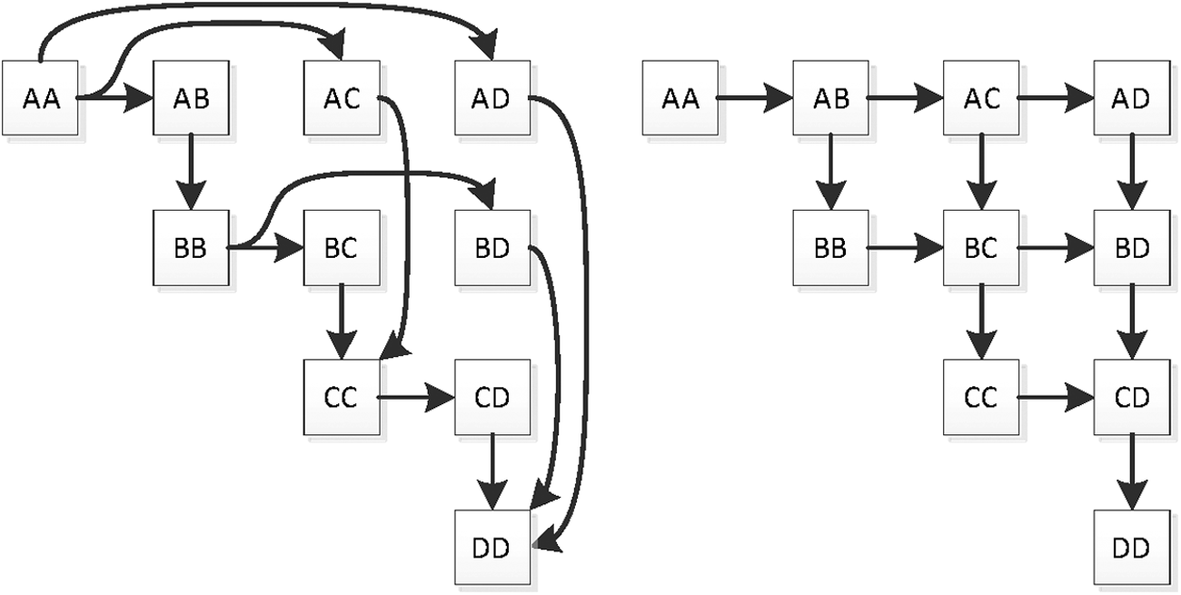
is monotonically increasing both along its rows and along its columns. Directional consistency and nonoverdominance can be expressed as partial orderings on the set of genotypes (given a fixed order of homozygotes), as illustrated in Figure 1.

OPEN IN VIEWER

FIG. 1.

Ordering relation constraints for single diploid locus. Left: no overdominance. Right: DCS. DCS, directional consistency of substitution.

2.2. Linearization and relaxed linearization

Both DCS and No Overdominance are implied by additivity and therefore necessary for the trait to be additive on some scale. From Figure 1, we immediately see that directional consistency implies No Overdominance and is therefore the stricter condition. The broader question is under what circumstances are these conditions sufficient for the existence of a natural scale. We can pose two forms of the natural scale problem. In the strict formulation, given a diploid trait with genotypic values \documentclass{aastex}\usepackage{amsbsy}\usepackage{amsfonts}\usepackage{amssymb}\usepackage{bm}\usepackage{mathrsfs}\usepackage{pifont}\usepackage{stmaryrd}\usepackage{textcomp}\usepackage{portland, xspace}\usepackage{amsmath, amsxtra}\pagestyle{empty}\DeclareMathSizes{10}{9}{7}{6}\begin{document} $${T_{ij}}$$ \end{document} on some arbitrary scale (e.g., on a rank scale from 1 to \documentclass{aastex}\usepackage{amsbsy}\usepackage{amsfonts}\usepackage{amssymb}\usepackage{bm}\usepackage{mathrsfs}\usepackage{pifont}\usepackage{stmaryrd}\usepackage{textcomp}\usepackage{portland, xspace}\usepackage{amsmath, amsxtra}\pagestyle{empty}\DeclareMathSizes{10}{9}{7}{6}\begin{document} $$\left( { \begin{matrix} n \\ 2 \\ \end{matrix}} \right) + \left( { \begin{matrix} n \\ 1 \\ \end{matrix}} \right) = \frac {{{n^2} + n}} {2} $$ \end{document} , the number of distinct genotypes for n alleles), is there a strictly increasing function \documentclass{aastex}\usepackage{amsbsy}\usepackage{amsfonts}\usepackage{amssymb}\usepackage{bm}\usepackage{mathrsfs}\usepackage{pifont}\usepackage{stmaryrd}\usepackage{textcomp}\usepackage{portland, xspace}\usepackage{amsmath, amsxtra}\pagestyle{empty}\DeclareMathSizes{10}{9}{7}{6}\begin{document} $$f$$ \end{document} such that there exists \documentclass{aastex}\usepackage{amsbsy}\usepackage{amsfonts}\usepackage{amssymb}\usepackage{bm}\usepackage{mathrsfs}\usepackage{pifont}\usepackage{stmaryrd}\usepackage{textcomp}\usepackage{portland, xspace}\usepackage{amsmath, amsxtra}\pagestyle{empty}\DeclareMathSizes{10}{9}{7}{6}\begin{document} $${\alpha _1} \ldots { \alpha _n}$$ \end{document} for which \documentclass{aastex}\usepackage{amsbsy}\usepackage{amsfonts}\usepackage{amssymb}\usepackage{bm}\usepackage{mathrsfs}\usepackage{pifont}\usepackage{stmaryrd}\usepackage{textcomp}\usepackage{portland, xspace}\usepackage{amsmath, amsxtra}\pagestyle{empty}\DeclareMathSizes{10}{9}{7}{6}\begin{document} \begin{align*} f \left( {{T_{ij}}} \right) = { \alpha _i} + { \alpha _j}. \end{align*} \end{document}

Counterexamples in Sverdlov and Thompson (In Prep) illustrate that a transformation to additivity is not always possible, even given directional consistency. A relaxed formulation of the problem is as follows: does there exist such a function f that is nondecreasing, but not trivially a constant? The constant valued function \documentclass{aastex}\usepackage{amsbsy}\usepackage{amsfonts}\usepackage{amssymb}\usepackage{bm}\usepackage{mathrsfs}\usepackage{pifont}\usepackage{stmaryrd}\usepackage{textcomp}\usepackage{portland, xspace}\usepackage{amsmath, amsxtra}\pagestyle{empty}\DeclareMathSizes{10}{9}{7}{6}\begin{document} $$f \left( \cdot \right) = c$$ \end{document} is always a nondecreasing solution; a nontrivial solution would vary over the domain of \documentclass{aastex}\usepackage{amsbsy}\usepackage{amsfonts}\usepackage{amssymb}\usepackage{bm}\usepackage{mathrsfs}\usepackage{pifont}\usepackage{stmaryrd}\usepackage{textcomp}\usepackage{portland, xspace}\usepackage{amsmath, amsxtra}\pagestyle{empty}\DeclareMathSizes{10}{9}{7}{6}\begin{document} $$f \left( \cdot \right)$$ \end{document} .

2.3. Traversal trees

The ordering constraint on the genotypes of a single locus system imposed by nonoverdominance or DCS, as in Figure 1, forms a directed acyclic graph (DAG), with genotype nodes and edges corresponding to each given constraint of the form \documentclass{aastex}\usepackage{amsbsy}\usepackage{amsfonts}\usepackage{amssymb}\usepackage{bm}\usepackage{mathrsfs}\usepackage{pifont}\usepackage{stmaryrd}\usepackage{textcomp}\usepackage{portland, xspace}\usepackage{amsmath, amsxtra}\pagestyle{empty}\DeclareMathSizes{10}{9}{7}{6}\begin{document} $$AA \prec AB$$ \end{document} . A fully specified trait corresponds to a complete ordering, and its DAG consists of a single connected path. Fixing the order of homozygotes with no loss of generality as \documentclass{aastex}\usepackage{amsbsy}\usepackage{amsfonts}\usepackage{amssymb}\usepackage{bm}\usepackage{mathrsfs}\usepackage{pifont}\usepackage{stmaryrd}\usepackage{textcomp}\usepackage{portland, xspace}\usepackage{amsmath, amsxtra}\pagestyle{empty}\DeclareMathSizes{10}{9}{7}{6}\begin{document} $$AA \prec BB \prec CC \prec DD$$ \end{document} , we can describe certain ordering constraints by an ordering constraint DAG as in Figure 1. The DAG corresponding to an ordering constraint is not generally unique. In particular, we can perform the transitive reduction (Aho et al., 1972) and transitive closure (Purdom, 1970) operations to find the minimal and maximal DAG, respectively. Equivalence of two ordering constraint DAGs is then given by the equivalence of their transitive closures. A fully specified trait corresponds to a complete ordering, and its DAG consists of a single connected path. Fixing the order of homozygotes with no loss of generality as \documentclass{aastex}\usepackage{amsbsy}\usepackage{amsfonts}\usepackage{amssymb}\usepackage{bm}\usepackage{mathrsfs}\usepackage{pifont}\usepackage{stmaryrd}\usepackage{textcomp}\usepackage{portland, xspace}\usepackage{amsmath, amsxtra}\pagestyle{empty}\DeclareMathSizes{10}{9}{7}{6}\begin{document} $$AA \prec BB \prec CC \prec DD$$ \end{document} , we can describe certain ordering constraints by an ordering constraint DAG as in Figure 1. The DAG corresponding to an ordering constraint is not generally unique. In particular, we can perform the transitive reduction Aho et al. (1972) and transitive closure Purdom (1970) operations to find the minimal and maximal DAG, respectively. Equivalence of two ordering constraint DAGs is then given by the equivalence of their transitive closures.

Any complete traversal of this DAG is an ordering of the nodes (genotypes) consistent with the ordering constraint, and therefore, a trait architecture. For example, \documentclass{aastex}\usepackage{amsbsy}\usepackage{amsfonts}\usepackage{amssymb}\usepackage{bm}\usepackage{mathrsfs}\usepackage{pifont}\usepackage{stmaryrd}\usepackage{textcomp}\usepackage{portland, xspace}\usepackage{amsmath, amsxtra}\pagestyle{empty}\DeclareMathSizes{10}{9}{7}{6}\begin{document} \begin{align*} AA \prec AD \prec AC \prec AB \prec BB \prec BC \prec BD \prec CC \prec CD \prec DD , \end{align*} \end{document}

is an ordering that satisfies nonoverdominance, but not DCS (e.g., \documentclass{aastex}\usepackage{amsbsy}\usepackage{amsfonts}\usepackage{amssymb}\usepackage{bm}\usepackage{mathrsfs}\usepackage{pifont}\usepackage{stmaryrd}\usepackage{textcomp}\usepackage{portland, xspace}\usepackage{amsmath, amsxtra}\pagestyle{empty}\DeclareMathSizes{10}{9}{7}{6}\begin{document} $$AC \prec AB$$ \end{document} but \documentclass{aastex}\usepackage{amsbsy}\usepackage{amsfonts}\usepackage{amssymb}\usepackage{bm}\usepackage{mathrsfs}\usepackage{pifont}\usepackage{stmaryrd}\usepackage{textcomp}\usepackage{portland, xspace}\usepackage{amsmath, amsxtra}\pagestyle{empty}\DeclareMathSizes{10}{9}{7}{6}\begin{document} $$BB \prec BC$$ \end{document} ).

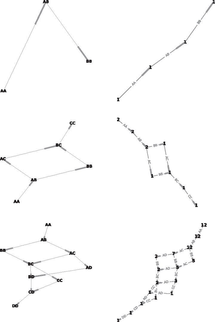
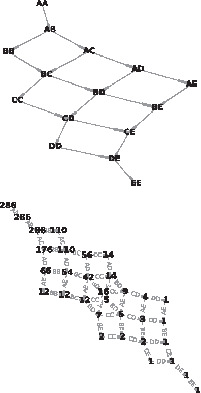
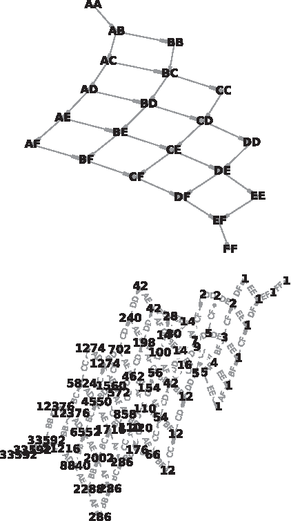
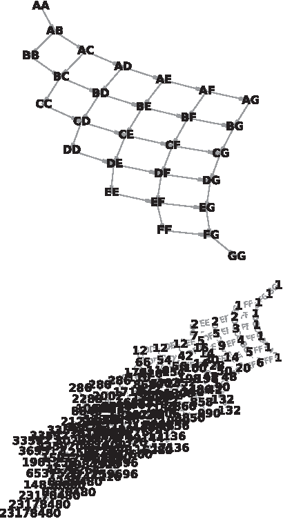
We developed an algorithm to transform the ordering constraint DAG to the Path DAG. This is a DAG with a single root and a single leaf. Each path from the root to the leaf corresponds to a traversal of the original DAG, with edges of the Path DAG corresponding to nodes of the original DAG (genotypes), and nodes of the Path DAG labeled with the number of distinct paths from that node to the leaf. This allows the enumeration, and therefore, counting and equally weighted sampling, of the paths through the original DAG. Figures 2 and 6 demonstrate the original and Path DAG for DCS for single locus diploid systems with between 2 and 7 alleles. The growth in number of directionally consistent orderings can be observed from the labeled number of paths from the root of the Path DAG.

OPEN IN VIEWER

FIG. 2.

Dominance patterns for \documentclass{aastex}\usepackage{amsbsy}\usepackage{amsfonts}\usepackage{amssymb}\usepackage{bm}\usepackage{mathrsfs}\usepackage{pifont}\usepackage{stmaryrd}\usepackage{textcomp}\usepackage{portland, xspace}\usepackage{amsmath, amsxtra}\pagestyle{empty}\DeclareMathSizes{10}{9}{7}{6}\begin{document} $$n = 2 , 3 , 4$$ \end{document} . Graph on the left is the allele ordering imposed on genotypes by DCS. Graph on the right is the Path DAG (Section 2.3). DAG, directed acyclic graph.

OPEN IN VIEWER

FIG. 6.

Dominance patterns for \documentclass{aastex}\usepackage{amsbsy}\usepackage{amsfonts}\usepackage{amssymb}\usepackage{bm}\usepackage{mathrsfs}\usepackage{pifont}\usepackage{stmaryrd}\usepackage{textcomp}\usepackage{portland, xspace}\usepackage{amsmath, amsxtra}\pagestyle{empty}\DeclareMathSizes{10}{9}{7}{6}\begin{document} $$n = 5$$ \end{document} .

The algorithm is analogous to the problem of generating, as in Pruesse and Ruskey (1994), or counting, as in Brightwell and Winkler (1991), the linear extensions in a DAG. Given an input DAG with allele set A and edges \documentclass{aastex}\usepackage{amsbsy}\usepackage{amsfonts}\usepackage{amssymb}\usepackage{bm}\usepackage{mathrsfs}\usepackage{pifont}\usepackage{stmaryrd}\usepackage{textcomp}\usepackage{portland, xspace}\usepackage{amsmath, amsxtra}\pagestyle{empty}\DeclareMathSizes{10}{9}{7}{6}\begin{document} $$a \to b$$ \end{document} representing ordering constraints of the form \documentclass{aastex}\usepackage{amsbsy}\usepackage{amsfonts}\usepackage{amssymb}\usepackage{bm}\usepackage{mathrsfs}\usepackage{pifont}\usepackage{stmaryrd}\usepackage{textcomp}\usepackage{portland, xspace}\usepackage{amsmath, amsxtra}\pagestyle{empty}\DeclareMathSizes{10}{9}{7}{6}\begin{document} $$a \prec b$$ \end{document} , the Path DAG we will generate will have nodes corresponding to subsets of \documentclass{aastex}\usepackage{amsbsy}\usepackage{amsfonts}\usepackage{amssymb}\usepackage{bm}\usepackage{mathrsfs}\usepackage{pifont}\usepackage{stmaryrd}\usepackage{textcomp}\usepackage{portland, xspace}\usepackage{amsmath, amsxtra}\pagestyle{empty}\DeclareMathSizes{10}{9}{7}{6}\begin{document} $$A$$ \end{document} :

1. Initialize the Path DAG to a single node, the empty set Ø.

OPEN IN VIEWER

FIG. 3.

Patterns of dominance, up to label permutation, for 2, 3, and 4 alleles. Solvable systems are in green; partially solvable in red.

Any path from A to Ø is then a distinct trait architecture, with the order found by collecting alleles from edge labels during the traversal. The path count assigned to node A is then the overall count of distinct trait architectures.

2.4. Natural scale recovery

Given a genotype ordering, for example \documentclass{aastex}\usepackage{amsbsy}\usepackage{amsfonts}\usepackage{amssymb}\usepackage{bm}\usepackage{mathrsfs}\usepackage{pifont}\usepackage{stmaryrd}\usepackage{textcomp}\usepackage{portland, xspace}\usepackage{amsmath, amsxtra}\pagestyle{empty}\DeclareMathSizes{10}{9}{7}{6}\begin{document} \begin{align*} AA \prec AB \prec BB \prec AC \prec BC \prec CC \end{align*} \end{document}

we can find numerical values for a natural scale, exactly or approximately, by a linear program. We will introduce three sets of variables:

1. Genotype variables: \documentclass{aastex}\usepackage{amsbsy}\usepackage{amsfonts}\usepackage{amssymb}\usepackage{bm}\usepackage{mathrsfs}\usepackage{pifont}\usepackage{stmaryrd}\usepackage{textcomp}\usepackage{portland, xspace}\usepackage{amsmath, amsxtra}\pagestyle{empty}\DeclareMathSizes{10}{9}{7}{6}\begin{document} $$AA , AB,BB,AC , BC , CC$$ \end{document}

The linear program then has the form

maximize \documentclass{aastex}\usepackage{amsbsy}\usepackage{amsfonts}\usepackage{amssymb}\usepackage{bm}\usepackage{mathrsfs}\usepackage{pifont}\usepackage{stmaryrd}\usepackage{textcomp}\usepackage{portland, xspace}\usepackage{amsmath, amsxtra}\pagestyle{empty}\DeclareMathSizes{10}{9}{7}{6}\begin{document} $$g_{AA}^{AB} + g_{AB}^{BB} + g_{BB}^{AC} + g_{AC}^{BC} + g_{BC}^{CC}$$ \end{document} subject to

This “accordion” linear program maximizes the number of gaps of the form \documentclass{aastex}\usepackage{amsbsy}\usepackage{amsfonts}\usepackage{amssymb}\usepackage{bm}\usepackage{mathrsfs}\usepackage{pifont}\usepackage{stmaryrd}\usepackage{textcomp}\usepackage{portland, xspace}\usepackage{amsmath, amsxtra}\pagestyle{empty}\DeclareMathSizes{10}{9}{7}{6}\begin{document} $$g_{AA}^{AB}$$ \end{document} , assigning the value of 1 to each strict inequality satisfied and 0 to each inequality relaxed into an equality. If it can, the program will make all inequalities strict; at worst, it will turn all inequalities into equalities, producing the trivial constant solution. The use of linear programming and optimization in translating order constraints to a cardinal scale can be traced to Kruskal (1964) and the development of the nonmetric version of the multidimensional scaling framework.

2.5. Solvability of dominance systems

We enumerated all possible single locus systems for 2, 3, and 4 alleles, up to permutation, and displayed the solutions as 3. For up to 4 alleles, all but two possible order architectures are solvable, that is, they have a natural scale that respects the strict inequalities of the ordering constraints. The two partially solvable orderings have relaxed or partial solutions; that is, they can be solved by turning some, but not all, or the strict inequalities into nonstrict inequalities. We tabulated results for higher numbers of alleles as Table 1. As the number of alleles rises, the fraction of architectures that either has relaxed solutions or no solutions increases.

3.1. Role of epistasis

The relative importance of epistasis, nonlinearity over multiple loci, in explaining the variability of quantitative traits remains controversial. A survey of the varied biological and statistical concepts of epistasis is given by Phillips (2008). In particular, we must distinguish between the noncontroversial assertion that epistasis in the biological sense, at the level of genes interacting to produce the phenotype of an individual, is common and the controversy around the relative importance of epistasis as a statistical phenomenon useful in describing variation at the population level. There is an ongoing debate between the advocates (Zuk et al., 2012) and critics (Hill et al., 2008) of an important role for epistatic genetic variance in general complex traits. The canonical example of a human anthropometric trait thought to have high epistatic genetic variance is the Total Dermal Ridge Count (Heath et al., 1984), a property of fingerprints. Fingerprints are typically nearly identical in monozygotic twins, but similarities between the fingerprints of other relatives do not follow a simple pattern. Thus, total genetic variance is high but additive variance is low, pointing to a big role for epistasis.

3.2. Directional consistency in epistasis

The concepts of the dominance framework developed above carry over directly to the case of epistasis over multiple loci, but the number of combinatorial cases and both the computational and notational difficulties increase considerably.

OPEN IN VIEWER

FIG. 7.

Dominance patterns for \documentclass{aastex}\usepackage{amsbsy}\usepackage{amsfonts}\usepackage{amssymb}\usepackage{bm}\usepackage{mathrsfs}\usepackage{pifont}\usepackage{stmaryrd}\usepackage{textcomp}\usepackage{portland, xspace}\usepackage{amsmath, amsxtra}\pagestyle{empty}\DeclareMathSizes{10}{9}{7}{6}\begin{document} $$n = 6$$ \end{document} .

OPEN IN VIEWER

FIG. 8.

Dominance patterns for \documentclass{aastex}\usepackage{amsbsy}\usepackage{amsfonts}\usepackage{amssymb}\usepackage{bm}\usepackage{mathrsfs}\usepackage{pifont}\usepackage{stmaryrd}\usepackage{textcomp}\usepackage{portland, xspace}\usepackage{amsmath, amsxtra}\pagestyle{empty}\DeclareMathSizes{10}{9}{7}{6}\begin{document} $$n = 7$$ \end{document} .

Consider a haploid organism with biallelic genotypes of k loci. The haploid genotype may be represented by a binary k-tuple with a genotypic value function of the form \documentclass{aastex}\usepackage{amsbsy}\usepackage{amsfonts}\usepackage{amssymb}\usepackage{bm}\usepackage{mathrsfs}\usepackage{pifont}\usepackage{stmaryrd}\usepackage{textcomp}\usepackage{portland, xspace}\usepackage{amsmath, amsxtra}\pagestyle{empty}\DeclareMathSizes{10}{9}{7}{6}\begin{document} $$f:{ \left\{ {0 , 1} \right\} ^n} \to { {\cal R}}$$ \end{document} , mapping the haploid genotype to genotypic value, such as the median phenotype without an environmental contribution. Where unambiguous, we will use the letter notation AbCDe or ACD for haploid genotype \documentclass{aastex}\usepackage{amsbsy}\usepackage{amsfonts}\usepackage{amssymb}\usepackage{bm}\usepackage{mathrsfs}\usepackage{pifont}\usepackage{stmaryrd}\usepackage{textcomp}\usepackage{portland, xspace}\usepackage{amsmath, amsxtra}\pagestyle{empty}\DeclareMathSizes{10}{9}{7}{6}\begin{document} $$\left( {1 , 0 , 1 , 1 , 0} \right)$$ \end{document} , and abcde or 0 for the specific haploid genotype \documentclass{aastex}\usepackage{amsbsy}\usepackage{amsfonts}\usepackage{amssymb}\usepackage{bm}\usepackage{mathrsfs}\usepackage{pifont}\usepackage{stmaryrd}\usepackage{textcomp}\usepackage{portland, xspace}\usepackage{amsmath, amsxtra}\pagestyle{empty}\DeclareMathSizes{10}{9}{7}{6}\begin{document} $$\left( {0 , 0 , 0 , 0 , 0} \right)$$ \end{document} . We assume a complete order on the haploid genotypes, as the possibility of ties is algebraically inconvenient. Without the loss of generality, we will order the loci and choose which alleles to call 1 or uppercase, so that \documentclass{aastex}\usepackage{amsbsy}\usepackage{amsfonts}\usepackage{amssymb}\usepackage{bm}\usepackage{mathrsfs}\usepackage{pifont}\usepackage{stmaryrd}\usepackage{textcomp}\usepackage{portland, xspace}\usepackage{amsmath, amsxtra}\pagestyle{empty}\DeclareMathSizes{10}{9}{7}{6}\begin{document} $$E \succ D \succ C \succ B \succ A \succ 0$$ \end{document} .

For the multilocus case, we must distinguish between weak (or first order) directional consistency and strong, complete, or general directional consistency. Intermediate order i directional consistency can also be defined.

Weak directional consistency is defined the invariance in the direction of the effect of the substitution at a single locus on the genotype at other loci. For example, if the substitution \documentclass{aastex}\usepackage{amsbsy}\usepackage{amsfonts}\usepackage{amssymb}\usepackage{bm}\usepackage{mathrsfs}\usepackage{pifont}\usepackage{stmaryrd}\usepackage{textcomp}\usepackage{portland, xspace}\usepackage{amsmath, amsxtra}\pagestyle{empty}\DeclareMathSizes{10}{9}{7}{6}\begin{document} $$c \to C \vert abde$$ \end{document} is positive, that is, if \documentclass{aastex}\usepackage{amsbsy}\usepackage{amsfonts}\usepackage{amssymb}\usepackage{bm}\usepackage{mathrsfs}\usepackage{pifont}\usepackage{stmaryrd}\usepackage{textcomp}\usepackage{portland, xspace}\usepackage{amsmath, amsxtra}\pagestyle{empty}\DeclareMathSizes{10}{9}{7}{6}\begin{document} $$abCde \succ abcde$$ \end{document} , then so is the substitution \documentclass{aastex}\usepackage{amsbsy}\usepackage{amsfonts}\usepackage{amssymb}\usepackage{bm}\usepackage{mathrsfs}\usepackage{pifont}\usepackage{stmaryrd}\usepackage{textcomp}\usepackage{portland, xspace}\usepackage{amsmath, amsxtra}\pagestyle{empty}\DeclareMathSizes{10}{9}{7}{6}\begin{document} $$c \to C \,\vert \,AbDe$$ \end{document} .

Order i directional consistency extends this to substitution at i loci at a time. For example, under second-order directional consistency, if the substitution \documentclass{aastex}\usepackage{amsbsy}\usepackage{amsfonts}\usepackage{amssymb}\usepackage{bm}\usepackage{mathrsfs}\usepackage{pifont}\usepackage{stmaryrd}\usepackage{textcomp}\usepackage{portland, xspace}\usepackage{amsmath, amsxtra}\pagestyle{empty}\DeclareMathSizes{10}{9}{7}{6}\begin{document} $$bD \to Bd \vert ace$$ \end{document} is positive, so is \documentclass{aastex}\usepackage{amsbsy}\usepackage{amsfonts}\usepackage{amssymb}\usepackage{bm}\usepackage{mathrsfs}\usepackage{pifont}\usepackage{stmaryrd}\usepackage{textcomp}\usepackage{portland, xspace}\usepackage{amsmath, amsxtra}\pagestyle{empty}\DeclareMathSizes{10}{9}{7}{6}\begin{document} $$bD \to Bd \,\vert\, aCE$$ \end{document} .

Strong directional consistency is directional consistency of all orders.

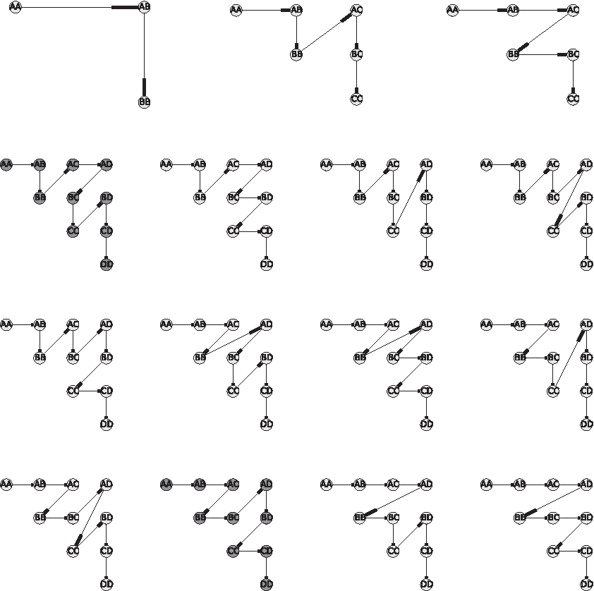
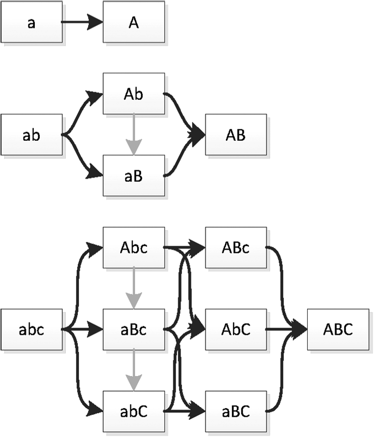
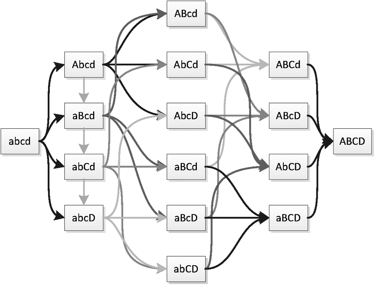
If the genotype is diploid, a single substitution may occur on either strand; thus, a diploid, single locus model with weak directional consistency is equivalent to the directional consistency model of dominance. Additivity implies strong directional consistency, and strong directional consistency implies weak directional consistency, but neither converse holds. Weak directional consistency as an ordering constraint can be represented as a DAG over genotypes for a fixed ordering of single “uppercase” locus genotypes, but strong directional consistency cannot. Directional consistency, in a relatively weak or strong form, is still a weaker and more biologically plausible hypothesis about a given trait than additivity. We plot the order constraints due to weak directional consistency as Figures 4 and 5.

OPEN IN VIEWER

FIG. 4.

Order constraints on epistatic systems with weak directional consistency for 1, 2, or 3 loci. Green indicates ordering of loci imposed by label permutation.

OPEN IN VIEWER

FIG. 5.

Order constraints on epistatic systems with weak directional consistency for 4 loci. Green indicates ordering of loci imposed by label permutation. Other colors arbitrary, for contrast only.

3.3. Algorithmic solutions

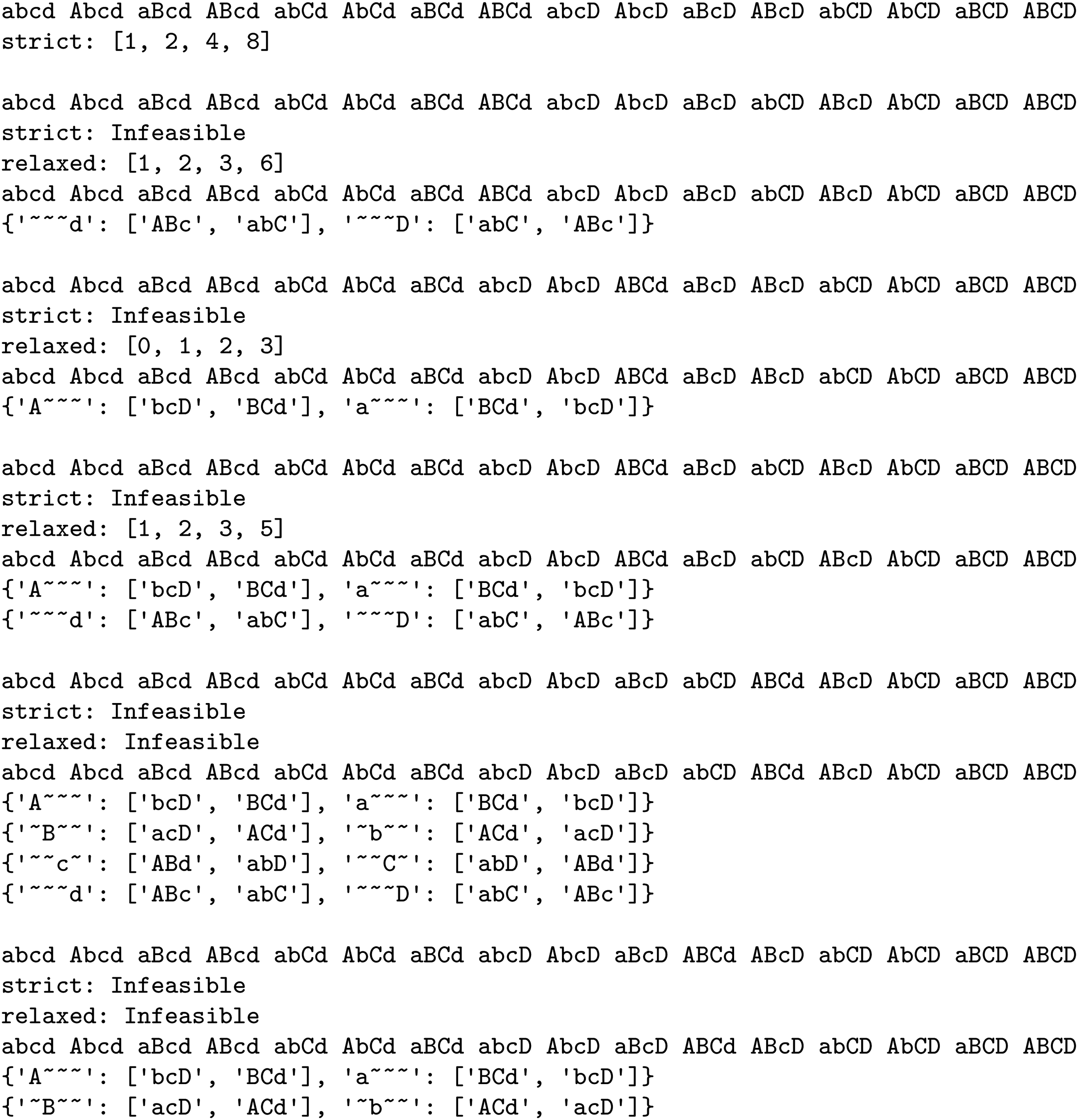
We developed an algorithm to solve epistatic order problems for natural scale, exactly or approximately, by linear programming, as well as to detect violations of directional consistency. For selected orderings, the output is illustrated as Fig. 9. As an example showing how to read this table, take the second block. The first row is an ordering of haploid genotypes in increasing order from abcd to ABCD. A strict solution, with no relaxation of strict inequalities, is impossible, but the maximum number of inequalities is satisfied in the best nontrivial solution, assigning \documentclass{aastex}\usepackage{amsbsy}\usepackage{amsfonts}\usepackage{amssymb}\usepackage{bm}\usepackage{mathrsfs}\usepackage{pifont}\usepackage{stmaryrd}\usepackage{textcomp}\usepackage{portland, xspace}\usepackage{amsmath, amsxtra}\pagestyle{empty}\DeclareMathSizes{10}{9}{7}{6}\begin{document} $$A = 1 , B = 2 , C = 3 , D = 6$$ \end{document} . The last row specifies the violation of directional consistency in the order given: conditioning on either d or D, the ordering or ABc and abC flips, a violation of third order consistency.

OPEN IN VIEWER

FIG. 9.

Output of violation classification algorithm.

The linear program is directly analogous to that used with the diploid (dominance) systems, with locus effect variables in place of allele effect variables. To find directional consistency violations, we enumerate the possibilities for a given ordering of genotypes:

1. For each nonempty subset S of loci: