A Computational Approach to Studying Protein Folding Problems Considering the Crucial Role of the Intracellular Environment

Abstract

Intracellular protein folding (PF) is performed in a highly inhomogeneous, crowded, and correlated environment. Due to this inherent complexity, the study and understanding of PF phenomena is a fundamental issue in the field of computational systems biology. In particular, it is important to use a modeled medium that accurately reflects PF in natural systems. In the current study, we present a simulation wherein PF is carried out within an inhomogeneous modeled medium. Simulation resources included a two-dimensional hydrophobic-polar (HP) model, evolutionary algorithms, and the dual site-bond model. The dual site-bond model was used to develop an environment where HP beads could be folded. Our modeled medium included correlation lengths and fractal-like behavior, which were selected according to HP sequence lengths to induce folding in a crowded environment. Analysis of three benchmark HP sequences showed that the modeled inhomogeneous space played an important role in deeper energy folding and obtained better performance and convergence compared with homogeneous environments. Our computational approach also demonstrated that our correlated network provided a better space for PF. Thus, our approach represents a major advancement in PF simulations, not only for folding but also for understanding functional chemical structure and physicochemical properties of proteins in crowded molecular systems, which normally occur in nature.

1. Introduction

Employment of computational approaches to study problems in science and engineering has been enhanced in the past decade through a multitude of techniques, including abstract interpretation, algorithms for computational biology, answer set programming, constraint-based programming, genome alignment, logical modeling of cellular networks, model checking, next-generation sequencing, Petri nets, phylogeny reconstruction, process algebras, rule-based modeling, evolutionary algorithms, ant-colony, stochastic simulation, symbolic methods (e.g., binary decision diagrams and the satisfiability problem solvers), systems biology, and so on (Vogel, 2002; Kaipio and Somersalo, 2004; Lodhi and Muggleton, 2010). This enhancement was also made possible by combining cross-disciplinary expertise in the fields of mathematics, physicochemical sciences, engineering, medicine, biology, and the social sciences, among others (Kitano, 2002; Omenn, 2006; Banga, 2008). The techniques suggested earlier have been employed to determine the cause(s) of complex phenomena in nature and to effectively simulate their conditions, which is a rather difficult task, since most phenomena are nonlinear in nature and the input data are often noisy or unclustered, of large scale, and possess high-dimensional spaces.

In the present study, we investigated problems regarding structural biology, specifically protein folding (PF). PF mechanisms are not yet clearly understood due to the inherent complexity of protein structures and their interactions with the surrounding environment. Therefore, this biological problem represents a challenge to computational simulation of intracellular processes. Levinthal stated this complexity in 1968 with his paradox (Levinthal, 1968). It is well known that the supramolecular self-assembly of amino acid sequences and the surrounding media should produce a well-defined three-dimensional (3D) shape; this happens because molecular entities are self-programmed or codified, giving place to the folded or native state of the protein.

In the past three decades, different modeling approaches have been developed to deal with PF. One common computational method is the coarse-grained minimalistic or hydrophobic-polar (HP) model, where amino acids are simply segregated as polar or hydrophobic constituents, because of its simplicity and predictive force (Dill, 1985; Unger and Moult, 1993; Gupta et al., 2005; Hoque et al., 2009). Nonetheless, only a few minimalistic models consider the crucial role of the intracellular environment in PF as a constrained or pressurized medium (Ping et al., 2003; Pattanasiri et al., 2013). We believe that experimental or theoretical crowding agents or parent contributions (e.g., pH, ionic strength, etc.) should be routinely added as controlling properties in computations to more accurately model the behavior of biological molecules in their natural environments (Luby-Phelps, 2000; Ellis, 2001; Minton, 2001; Ellis and Minton, 2003).

Although there is a strong correlation between the primary amino acid sequence and structure of polymeric protein chains, the intracellular environment is also known to induce the native state structure and provoke changes in protein shape. In other words, the crowded medium inside cells directly affects PF (van den Berg et al., 1999; Homouz et al., 2008; Munishkina et al., 2008; Mittal and Singh, 2014). Hence, the purpose of the current study was to model PF through the folding of HP sequences, taking into account inhomogeneous (fractal) characteristics of the surrounding environment. Here, we propose to mimic the environment that surrounds amino acid sequences in a real system during the PF process.

In Section 2, we briefly explain the folding space by using the dual site-bond model (DSBM). In Section 3, we present our bioinformatics platform, named Evolution, a computational algorithm for folding HP sequences in both homogenous and inhomogeneous media. Then, in Section 4, we discuss the development of three studies involving the folding of three complex HP sequences in both homogenous and inhomogeneous environments. Finally, Section 5 includes a discussion of the results of our simulations.

2. Modeling of Inhomogeneous Space Through DSBM

In our study, we perform HP sequence folding simulations in both homogeneous and inhomogeneous networks. The inhomogeneous space was designed to be correlated and fractal like to try and mimic the environment that surrounds amino acid sequences in real systems during PF processes (Aon and Cortassa, 1994; Kurakin, 2011; Vasilescu et al., 2013). This medium was built with a DSBM used in a previous work to fold some HP sequences. Although the DSBM is described in detail elsewhere, we discuss the main aspects needed to understand our results (Alas and González-Pérez, 2016).

A network can be formed by two kinds of alternating elements: sites and bonds. In certain lattice configurations, bonds connect sites. In square lattices, sites are located at lattice nodes, whereas bonds are located between two adjacent sites; thus, two sites delimit each bond, whereas each site is associated with four bonds, and, therefore, site connectivity dimension is four. Figure 1 shows a schematic representation of a two-dimensional (2D) network of L × L sites and 2L × L bonds, where L = 4 sites.

FIG. 1.

(a) Schematic representation of a network in 2D generated from sites and bonds. The bonds in dotted lines represent the periodic boundary conditions used in all simulations. (b) A site connected by four bonds; the R_S and R_B radius are shown.

For the inhomogeneous networks, the size of each element was simply expressed by means of a “metric” R, which was defined as follows: For sites considered hollow spheres, R_S is the radius of the sphere, whereas for bonds considered hollow cylinders, R_B is the radius of the cylinder, in this case, half the bond width (Fig. 1). Therefore, these networks are constructed from the distribution functions S(R) and B(R), such that: \documentclass{aastex}\usepackage{amsbsy}\usepackage{amsfonts}\usepackage{amssymb}\usepackage{bm}\usepackage{mathrsfs}\usepackage{pifont}\usepackage{stmaryrd}\usepackage{textcomp}\usepackage{portland, xspace}\usepackage{amsmath, amsxtra}\usepackage{upgreek}\pagestyle{empty}\DeclareMathSizes{10}{9}{7}{6}\begin{document} \begin{align*} S \left( R \right) = \int_0^R {{F_{ \rm{S}}} \left( {{R_{ \rm{S}}}} \right) d{R_{ \rm{S}}}} { \rm{;}} \quad \quad \quad B \left( R \right) = \int_0^R {{F_{ \rm{B}}} \left( {{R_{ \rm{B}}}} \right) d{R_{ \rm{B}}}} , \tag{1} \end{align*} \end{document}

where F_S(R_S) and F_B(R_B) are the corresponding probability density functions. The sites and bonds are connected to form the network through the joint probability density function, F(R_S, R_B). This connection follows the “construction principle,” which expresses the fact that the size of any bond R_B is always smaller, or at least equal, than the size of the R_S site. This law can be expressed locally as follows: \documentclass{aastex}\usepackage{amsbsy}\usepackage{amsfonts}\usepackage{amssymb}\usepackage{bm}\usepackage{mathrsfs}\usepackage{pifont}\usepackage{stmaryrd}\usepackage{textcomp}\usepackage{portland, xspace}\usepackage{amsmath, amsxtra}\usepackage{upgreek}\pagestyle{empty}\DeclareMathSizes{10}{9}{7}{6}\begin{document} \begin{align*} F \left( {{R_{ \rm{S}}} , {R_{ \rm{B}}}} \right) { \rm{ = 0}} \quad { \rm{if}} \quad {R_{ \rm{S}}} < {R_{ \rm{B}}} \quad { \rm{otherwise}} \quad F \left( {{R_{ \rm{S}}} , {R_{ \rm{B}}}} \right) { \rm{ > 0}}. \tag{2} \end{align*} \end{document}

The probability density for this joint event to occur is: \documentclass{aastex}\usepackage{amsbsy}\usepackage{amsfonts}\usepackage{amssymb}\usepackage{bm}\usepackage{mathrsfs}\usepackage{pifont}\usepackage{stmaryrd}\usepackage{textcomp}\usepackage{portland, xspace}\usepackage{amsmath, amsxtra}\usepackage{upgreek}\pagestyle{empty}\DeclareMathSizes{10}{9}{7}{6}\begin{document} \begin{align*} F \left( {{R_{ \rm{S}}} , {R_{ \rm{B}}}} \right) = {F_{ \rm{S}}} \left( {{R_{ \rm{S}}}} \right) {F_{ \rm{B}}} \left( {{R_{ \rm{B}}}} \right) \Phi \left( {{R_{ \rm{S}}} , {R_{ \rm{B}}}} \right) , \tag{3} \end{align*} \end{document}

where the correlation function Φ(R_S,R_B) includes information about the site-bond assignment procedure within the network. In natural forms, an overlapping area Ω appears between the site and bond probability density functions (Fig. 2). Therefore, Ω is a fundamental parameter describing the topology of the network. However, a physically more meaningful parameter is the correlation length (ξ), which is directly related to Ω. Therefore, if Ω = 0, then ξ = 0, which is the condition for a completely random network. In comparison, if Ω = 1, then ξ ≈ ∞; this condition corresponds to the homogeneous network modeled. For the desired, correlated network, it must be situated among these ranges: ξ → 0 for Ω → 0 and ξ → ∞ for Ω → 1.

FIG. 2.

Uniform probability density functions for sites (solid line) and bonds (dotted line). The shaded area depicts the overlap Ω between the distributions. F_B and F_S are defined at the range b = [b₁, b₂) and s = [s₁, s₂), respectively.

Understanding the latter, to mimic the intracellular space, classical percolation spanning clusters were constructed across each correlated network, which are characterized by different ξ values. These structures were generated by a classical percolation algorithm (Hoshen and Kopelman, 1976). Thus, for each network, the critical site-percolation threshold (ρ) was determined. Moreover, the structural irregularity of the percolation clusters was measured by means of the fractal dimension (d_f), by using the box-counting method (Alas and González-Pérez, 2016). Figure 3a and b show a correlated network of L × L sites, in this case L = 1000 sites (L = net length; thus, 1 × 10⁶ sites are represented), and the corresponding percolation cluster, respectively.

FIG. 3.

(a) Graphical representation of a correlated network generated from DSBM and (b) the corresponding classical site percolation structure of an infinite cluster obtained by Monte Carlo simulation. The main values are: Ω = 0.875, ξ = 11.70, ρ = 0.5023, and d_f = 1.764. DSBM, dual site-bond model.

3. The Evolution Bioinformatics Tool

The earlier version of our bioinformatics tool Evolution presented and discussed previously (Beltrán et al., 2009; González et al., 2009; Cervantes-Ojeda et al., 2010) was devoted to the study of PF with the HP model and a bead-like description of the chain; herein, our platform was augmented with the DSBM. Evolution allows to induce folding of molecular-chain representations with the aim of exploring both the efficiency of HP and the evolutionary algorithm technique and the effectiveness of DSBM for the representation of the intracellular space.

3.1. Algorithmic and representational aspects in Evolution

3.1.1. The 2D/3D HP representation

Evolution uses a 2D and 3D HP model (Shmygelska and Hoos, 2005) for the representation and folding of amino acid sequences. The chain described by the HP model can fold in simplistic 2D/3D space or Cartesian axes, and discrete movements of each bead of the sequence are fitted into a cell or lattice mimicking PF (for further details, see Alas and González-Pérez, 2016).

3.1.2. Search and optimization of 2D/3D structures

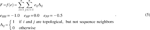
The search and optimization processes of HP structures were carried out by a genetic algorithm (GA) (Goldberg, 1989; Mitchell, 1999) that was used to search through the conformational space to find the structural shape that best meets the criteria established in the fitness function (i.e., optimization function). A commonly used criterion based on a thermodynamic hypothesis is to find the global minimum energy conformation (Unger and Moult, 1993; Patton et al., 1995; König and Dandekar, 1999; Cox et al., 2004), characterized by forming a core of hydrophobic (H) beads, whereas polar (P) beads are exposed to the outside of any conformation. Figure 4 shows some examples of these global minimum energy conformations in 2D/3D lattices.

FIG. 4.

Examples of global minimum energy conformations in standard 2D/3D lattices. H fragments are represented as dark gray beads, and P fragments are represented as light gray beads. These conformations were generated in the Evolution framework and have optimal scores of (a) 9, (b) 15, and (c) 28, taking into account only H···H interactions.

It should be mentioned that employment of GA represents an exhaustive search, considering a GA provides approximate solutions to optimization problems. Therefore, the exploration is directly related to the dimension and characteristics of the selected sample space, in this case, the initial population. Although best solutions for these selected criteria were found, they are not the best solution for the general problem, because it depends on many variables. Therefore, to try and find the best known solution of a given HP sequence, any user of Evolution should explore these criteria.

3.1.3. Optimization functions

The optimization function in Evolution can be defined in different ways, including all types of scoring, energy interaction terms, biophysicochemical information, and/or receive feedback from the GA during the optimization procedure. Equations (4) and (5) describe two models of optimization functions implemented in Evolution. On the other hand, Equation (6) denotes a novel model of the optimization function under study, considering two important measures of conformation compactness: radius of gyration (Equation (7)) and final average maximal diameter (Equation (8)); both are useful for analyzing the resulting 2D/3D conformations.

Model 1: There is a just minimum energetic reward for H···H interactions (e_HH).

Model 2: There is also a reward for P···P interactions (e_PP).

Model 3 (not yet implemented for optimization in Evolution): Radius of gyration (R_g) and final average maximal diameter (D_max) are considered as follows: \documentclass{aastex}\usepackage{amsbsy}\usepackage{amsfonts}\usepackage{amssymb}\usepackage{bm}\usepackage{mathrsfs}\usepackage{pifont}\usepackage{stmaryrd}\usepackage{textcomp}\usepackage{portland, xspace}\usepackage{amsmath, amsxtra}\usepackage{upgreek}\pagestyle{empty}\DeclareMathSizes{10}{9}{7}{6}\begin{document} \begin{align*} F = H \left( \,{f \left( e \right) , \ {R_g} , \ {D_{ \max }}} \right) , \tag{6} \end{align*} \end{document}

where f (e) can be defined as in Model 1 or in Model 2. \documentclass{aastex}\usepackage{amsbsy}\usepackage{amsfonts}\usepackage{amssymb}\usepackage{bm}\usepackage{mathrsfs}\usepackage{pifont}\usepackage{stmaryrd}\usepackage{textcomp}\usepackage{portland, xspace}\usepackage{amsmath, amsxtra}\usepackage{upgreek}\pagestyle{empty}\DeclareMathSizes{10}{9}{7}{6}\begin{document} \begin{align*} { R_g } = \sqrt { \frac { 1 } { N } } \sum \limits_ { k = 1 } ^N { { { \left( { { r_k } - { r_ { mean } } } \right) } ^2 } } \quad \quad \forall { r_k } \quad k = 1 , 2 , \ldots , N , \tag { 7 } \end{align*} \end{document}

where r_k = (x_k, y_k) for 2D conformations, r_k = (x_k, y_k, z_k) for 3D conformations, and r_mean is the mean position of the molecules, and \documentclass{aastex}\usepackage{amsbsy}\usepackage{amsfonts}\usepackage{amssymb}\usepackage{bm}\usepackage{mathrsfs}\usepackage{pifont}\usepackage{stmaryrd}\usepackage{textcomp}\usepackage{portland, xspace}\usepackage{amsmath, amsxtra}\usepackage{upgreek}\pagestyle{empty}\DeclareMathSizes{10}{9}{7}{6}\begin{document} \begin{align*} {D_{{ \rm{max}}}} = \max \left( {{d_{ij}}} \right) \quad \quad \forall {r_i} , {r_j} \quad i , j = 1 , 2 , \ldots , N , \tag{8} \end{align*} \end{document}

where \documentclass{aastex}\usepackage{amsbsy}\usepackage{amsfonts}\usepackage{amssymb}\usepackage{bm}\usepackage{mathrsfs}\usepackage{pifont}\usepackage{stmaryrd}\usepackage{textcomp}\usepackage{portland, xspace}\usepackage{amsmath, amsxtra}\usepackage{upgreek}\pagestyle{empty}\DeclareMathSizes{10}{9}{7}{6}\begin{document} $${d_{ij}} = d \left( {{r_i} , \ {r_j}} \right)$$ \end{document} .

3.1.4. Types of conformational spaces, conformations, and connectivity

Evolution provides two types of space for sequence folding: homogeneous space (the standard lattice introduced in Section 3.1.1) and inhomogeneous space (the DSBM introduced in Section 2). In the homogenous space, 2D and 3D sequence folding can be carried out. In the inhomogeneous space, only 2D sequence folding is implemented. The types of connectivity (i.e., the underlying geometry in creating conformations) allowed are 2D-Square, 2D-Triangle, and 3D-Cubic. Figure 5 shows the types of conformational spaces, conformations, and connectivity supported by Evolution.

FIG. 5.

Types of conformational spaces, conformations, and connectivity supported by Evolution. (a) Homogeneous space with a 2D square conformation, (b) Homogeneous space with a 2D triangle conformation, (c) Homogeneous spaces with a 3D cubic conformation, and (d) Inhomogeneous spaces with 2D square conformation.

3.1.5. The GA

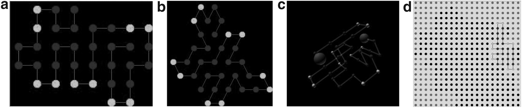
The version of the GA implemented in Evolution uses the following types of operators at each step to create the next population of 2D protein structures from the current population: selection, elitism, crossover, mutation, and migration. In detail, the main steps performed by the GA for searching and optimization of 2D protein structures are summarized later and illustrated in Figure 6.

FIG. 6.

Main steps performed by the GA implemented in Evolution tool. Steps 4.1–4.3 represent the GA cycle fitness-selection-crossover-mutation. Dotted arrows indicate conditionals (see steps 5–7 of the GA). GA, genetic algorithm.

1. Set parameter values for the size of the initial population (i.e., number of 2D protein structures to be generated from the target HP sequence—this is the sample space), the maximum number of iterations (N), and optimal expected value (OV), if known.

2. Set parameter values for selection, elitism, crossover, mutation, and migration operators.

3. Generation of the initial population of 2D protein structures from the target HP sequence according to the geometric model, in this case 2D HP.

4. Repeat the following steps N times or until OV is reached:

4.1. Evaluation of the fitness function for all 2D protein structures as stated by Equations (4) and (5).

4.2. Apply the selection and elitism operators for creating a set of parents. Comment: Parents (i.e., 2D protein structures) are selected to mate based on their fitness.

4.3. Apply the crossover and mutation operators to create a new population of 2D protein structures.

5. If the OV was reached, proceed to step 8.

6. If there is any evidence of a premature convergence, then apply the migration operator and go to step 4.

Comment: The migration operator replaces a number (N) of selected 2D protein structures by N new 2D protein structures generated randomly. This can be seen as the introduction of “new genetic material” to raise the search and optimization processes, preserving the results achieved.

7. If tuning parameters are required, go to step 1.

8. Finish.

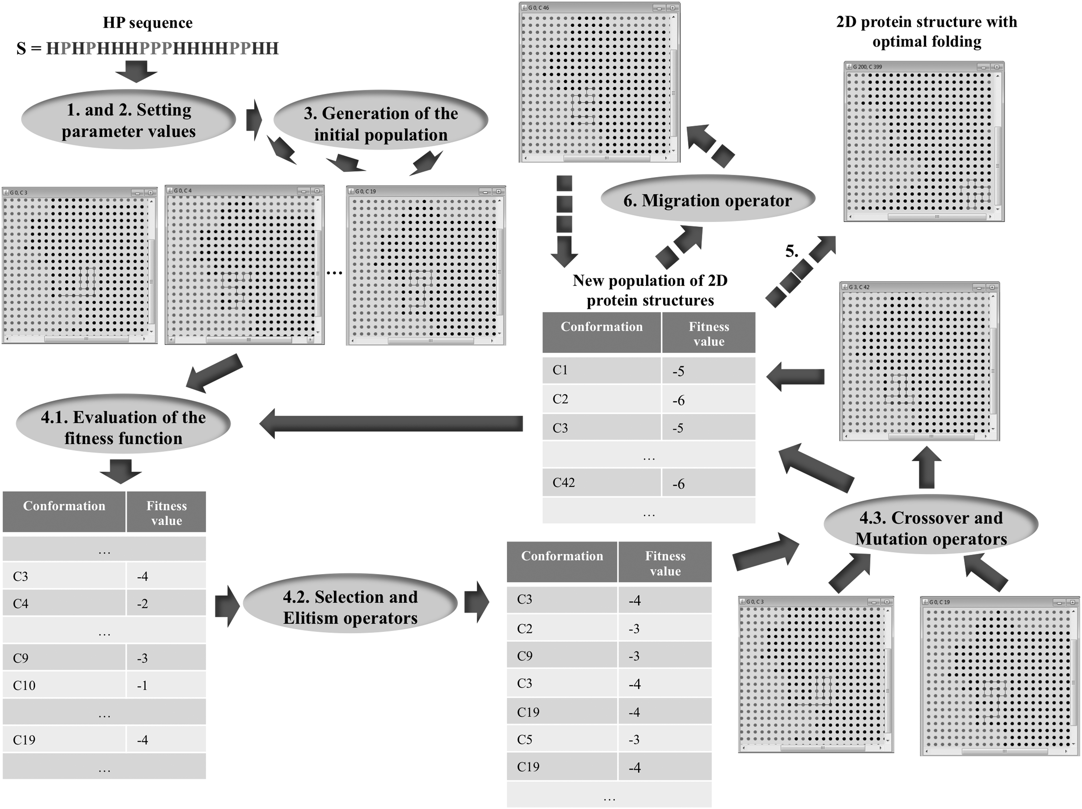
3.2. Evolution workflow

Carrying out the running experiments on Evolution is a straightforward process. Figure 7 shows the workflow of the major activities to be executed through Evolution when simulating the PF problem; the reader is referred to related references (Beltrán et al., 2009; González et al., 2009; Cervantes-Ojeda et al., 2010; Alas and González-Pérez, 2016). As we will see in the next section, this article focuses primarily on the role played by the representation of the intracellular space in the folding of the HP sequences.

FIG. 7.

Evolution workflow. The activity diagram describes the sequence of the major activities carried out during the folding simulation.

3.3. Application accessibility

The Evolution bioinformatics tool (in its Executable Jar File version) and the simulation file can be downloaded from the bioinformatics website of our research group at http://bioinformatics.cua.uam.mx/node/9. It should be noted that Evolution was developed as a stand-alone application and not as a Web application; for proper installation, follow the instructions included in the README file.

4. Results and Discussion

To address how the Evolution bioinformatics platform works and how the intracellular space might affect PF, we assessed the 2D HP model in (1) a square homogeneous space where the spatial correlation among elements was infinite and there was no fractal dimension, meaning that each element of the network had the same value (e.g., the sites had the same size); this occurs because a structure on the lattice was not formed, and (2) a square inhomogeneous network with different degrees of spatial correlation and fractal dimension, meaning that the network elements were different (e.g., the size of the sites varied); in this case, a structure was formed on the lattice (Fig. 3). To make a comparison and evaluate the effects of the homogeneous and inhomogeneous environments on the folding of the HP sequences, we carried out an analysis of three benchmark sequences for this model.

Table 1 shows the HP sequences analyzed in the present work. Sequences 1 and 2 (S1, S2) have been taken from the contributions of Unger and Moult (1993) and Thachuk et al. (2007). Moreover, S2 was previously tested by König and Dandekar (1999), as well as by Liang and Wong (2001); they reported the minimum energy and the structural ground conformation of this sequence. However, sequence 3 (S3) was taken from Huang et al. (2010).

Table 1.

Standard Benchmark Sequences

Sequence	Length	Optimal fitness	2D HP sequences
S1	36	−14	P₃H₂P₂H₂P₅H₇P₂H₂P₄H₂P₂HP₂
S2	48	−23	P₂H(P₂H₂)₂P₅H₁₀P₆(H₂P₂)₂HP₂H₅
S3	60	−36	P₂H₃PH₈P₃H₁₀PHP₃H₁₂P₄H₅PH₂PHP

HP, hydrophobic-polar.

4.1. Step-by-step HP sequence folding in an inhomogeneous space of a correlated network type

To better illustrate Evolution's operation, next we describe the main steps carried out during the folding of S1 in an inhomogeneous space through just 10 experiments for homogeneous/inhomogeneous space comparison purposes, but not the exhaustive finding of general solutions.

Step 1: As shown in Figure 8, the first step includes introduction of the HP sequence (see text box “Amino acid or HP sequence” at the top of the Graphical User Interface and the selection of the “Space Types” for folding it). As seen in Figure 9, the inhomogeneous space, mimicked as a correlated network, was selected. Since the only inhomogeneous space currently implemented in the tool is the one identified as “Correlated 2D Square” (Fig. 9), we selected this.

FIG. 8.

Step 1: GUI of Evolution bioinformatics tool. Introduction of the HP sequence and selection of the type of folding space. As can be seen in the “Space Types” panel, the correlated network has been selected as folding space. GUI, graphical user interface; HP, hydrophobic-polar.

FIG. 9.

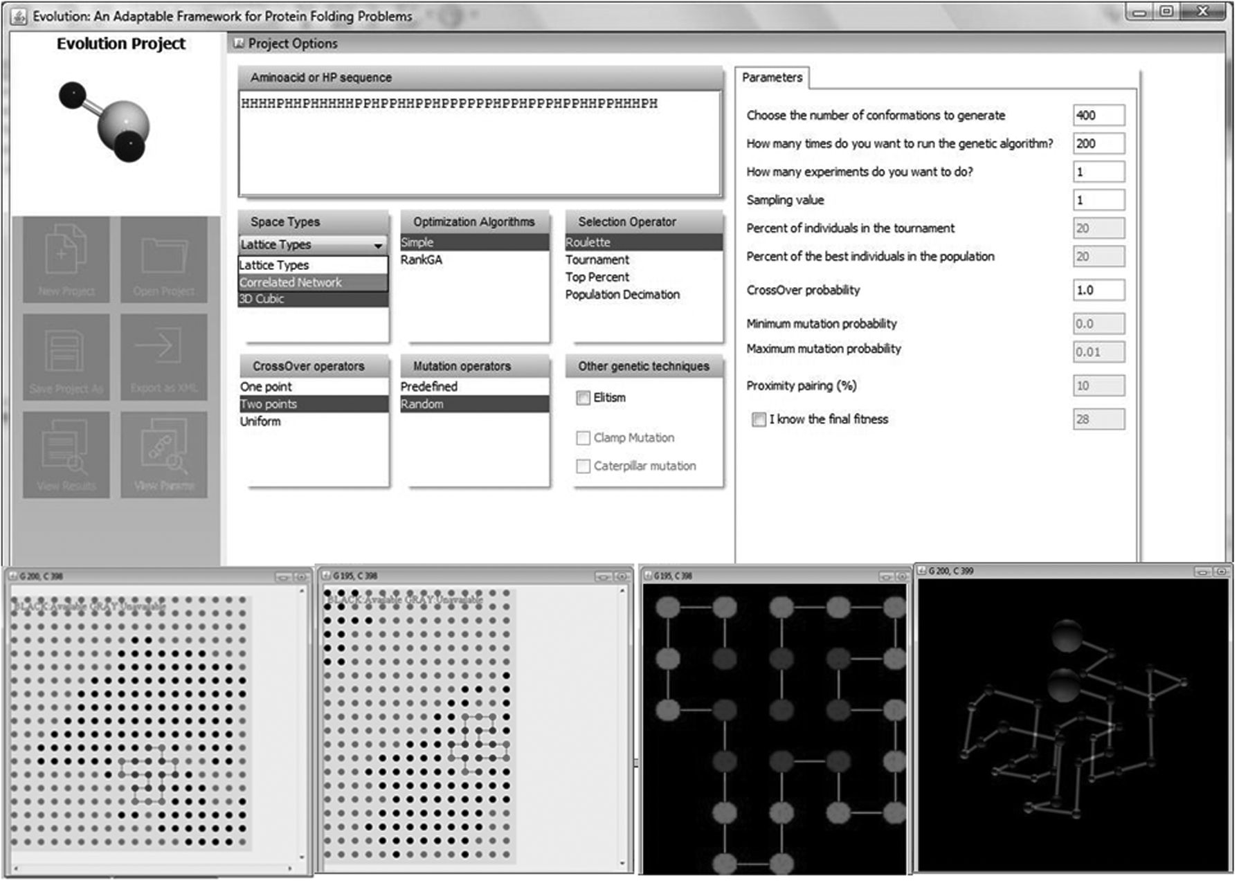
The main GUI of Evolution framework showing types of folding space: inhomogeneous (below left), homogeneous (below right), and some conformations created.

Step 2: As a result, the tool shows all available correlated networks (Fig. 10). Note that each of these correlated networks is characterized by a particular correlation length ξ. Here, a correlated network with ξ = 11.70 was selected (right part of Fig. 10), as it was intermediate among the correlated networks that were constructed ξ = 0.94, 1.80, 3.34, 5.58, 11.70, 18.12, 28.24, and 37.98. This implies that the homogeneity radial area for the latter ξ should be approximately 1, 2, 3, 6, 12, 18, 28, and 38 sites, respectively. Therefore, the folding of sequences should be considerably different depending on the ξ. We selected ξ = 11.70 because with longer values, the area of homogeneity is too big to achieve induction of folding phenomena for the sizes of sequences selected herein. Furthermore, with shorter values, any of the sequences would be too difficult to fold, because the high amount of obstacles present due to the high heterogeneity in the percolation cluster to fold such a sequence.

FIG. 10.

Step 2: visualization of all available correlated networks and selection of the required network for PF. Note that, as introduced in Section 2, each of these correlated networks is characterized by a particular correlation length ξ. As can be seen in the right part of this figure, we have selected the correlated network with correlation length ξ = 11.70. PF, protein folding.

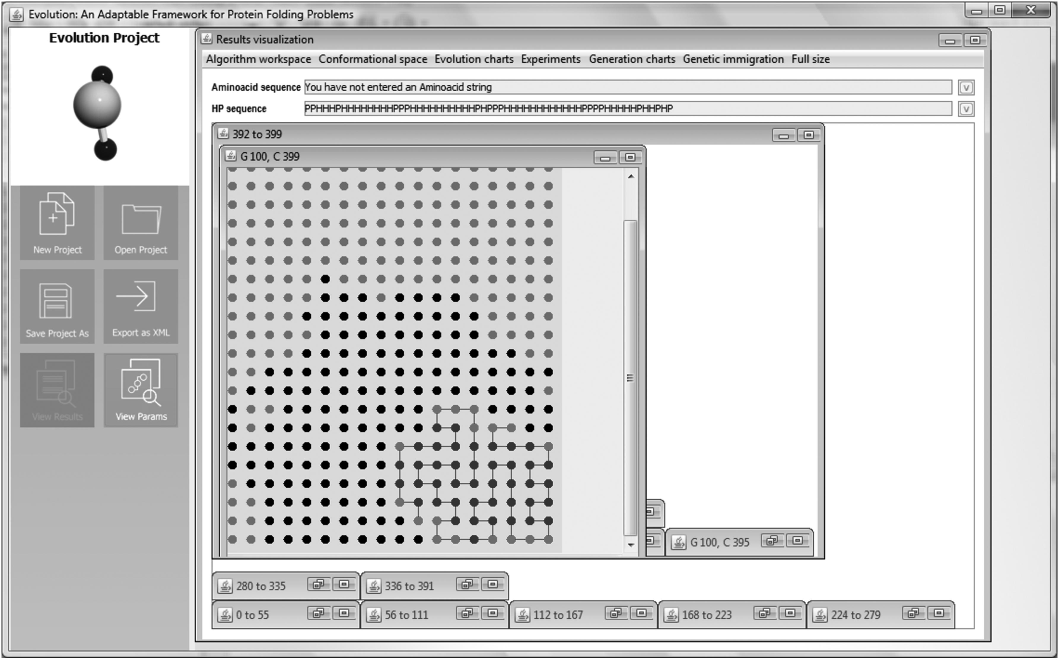
Step 3: After selecting the correlated network, we proceeded to identify the region (i.e., a cluster grain) in which to perform HP sequence folding. As shown on the right side of Figure 11, Evolution offers the user a tool palette for selection and editing of the required grain as a gray selection box. Figures 11 and 12 show the selected grain, where the folding of the HP sequence is carried out. As shown in Figure 12, the defined region for HP sequence folding is represented by black dots and enclosed by gray dots, the latter representing the absence of space for folding.

FIG. 11.

Step 3: identification and selection of the region (i.e., the grain) in which the folding of the HP sequence will be accomplished. As can be seen on the right side of this figure, Evolution offers the user a tool palette for selection and editing of the grain required as a gray selection box.

FIG. 12.

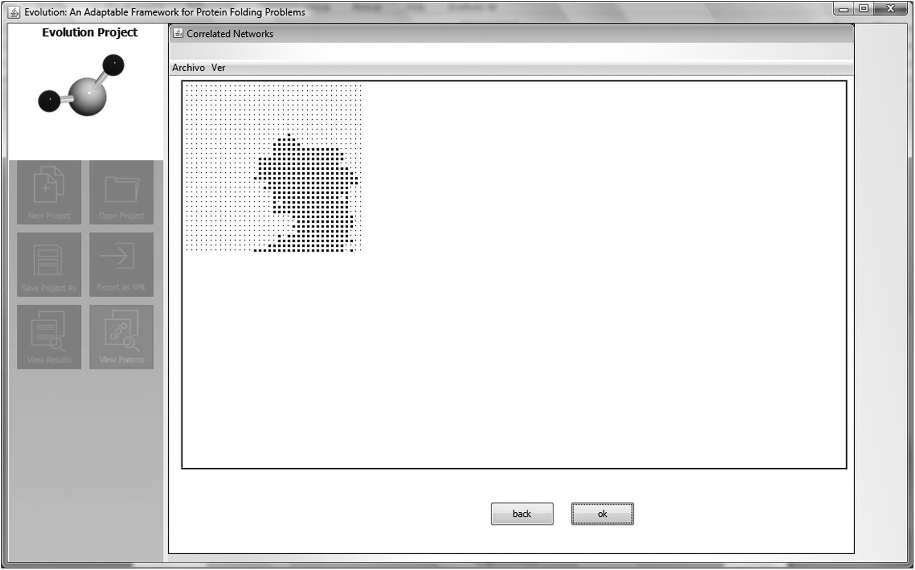
Step 3: The region (i.e., the fragment of the correlated network) for the folding of HP sequence that has been selected.

Step 4: Next, we set the parameters of the folding algorithm. As shown in the right panel of Figure 13, 10 experiments were executed, each with an initial population of 400 randomly generated conformations folded on the selected grain (Fig. 11). In each experiment, the folding algorithm ran a cycle consisting of 200 iterations. The left panel in Figure 13 shows assignment of values for other parameters required by the folding algorithm.

FIG. 13.

Step 4: setting folding algorithm parameters. As shown in the “Parameters” panel, 10 experiments will be executed, each one with an initial population of 400 randomly generated conformations folded on the selected grain and shown in Figure 12. In each experiment, the folding algorithm will run a cycle consisting of 200 iterations. The left panel shows the assignment of values for other parameters required by the folding algorithm.

Step 5: After assignment of values for parameters, the folding algorithm starts its execution. Table 2 shows the results obtained for S1 from 10 experiments carried out on the selected grain (Fig. 12). Table 2 shows it was possible to find the optimum energy value (−14) in two of the 10 experiments (i.e., experiments 3 and 7). In addition, in another three experiments, a value very close to the optimum was reached (i.e., experiments 2, 5, and 8), with a final score of −13. We analyzed these results together with those obtained during folding of S1 in the homogeneous space.

Table 2.

Dataset from 10 Experiments

	Experiments
Results	1	2	3	4	5	6	7	8	9	10
Highest score	−11	−13	−14	−11	−13	−11	−14	−13	−11	−12
Final score	−11	−13	−14	−11	−13	−11	−14	−13	−11	−12
R_gf	3.45	3.28	3.08	2.93	3.28	3.16	3.12	3.28	2.93	3.67
D_maxf	11.49	10.42	10.23	9.73	10.42	9.95	10.95	10.42	10.11	11.39

Results obtained for the folding of sequence S1 from 10 experiments carried out on an inhomogeneous space (i.e., on the grain selected in Fig. 11). As specified in Figure 13, the size of the population (no. of conformations) of each experiment is 400 and the number of generations is 200, where R_gf is the final average radius of gyration and D_maxf is the final average maximal diameter.

Figures 14 –16 show the progress and results of experiment 7 where the optimal score of −14 was achieved. Figure 14 shows the behavior of the score (i.e., average, best, and worst scores) through 200 generations. Note that the optimal fitness (represented on the graph by a yellow line) is reached at an early stage of the experiment and maintained through all subsequent generations. In Figure 15, we can see the behavior of radius of gyration and maximal diameter through 200 generations or iterations. Figure 16 shows an optimal conformation (i.e., a conformation with an optimal score) belonging to generation 180. Note that this conformation was generated exactly in the borders of the region or selected grain, allowing appreciation of the role of correlated space in the folding sequence.

FIG. 14.

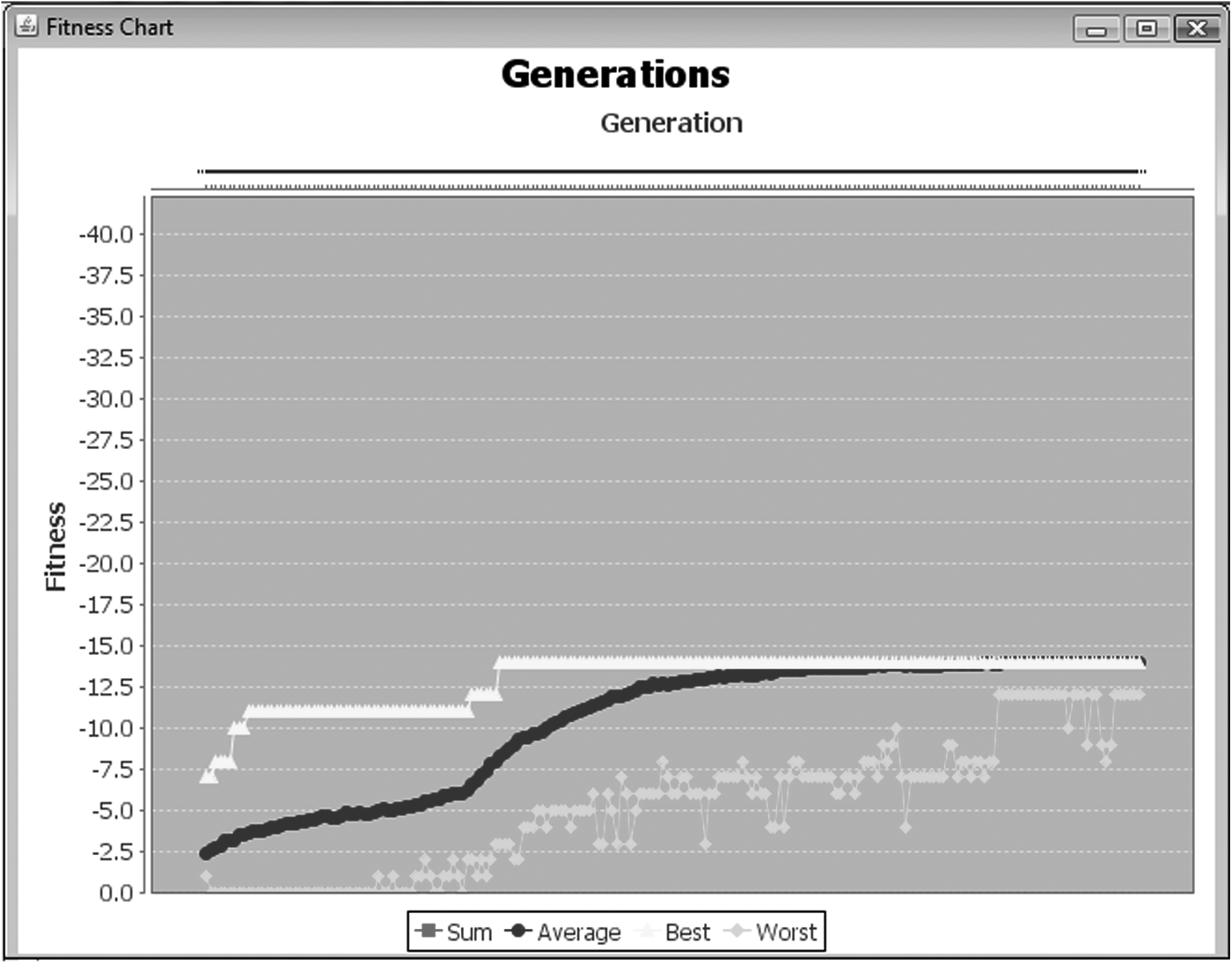
Behavior of the score: average score, best score, and worst score, through 200 generations or iterations for the experiment number 7. On the chart, the x-axis represents the generations and the y-axis represents the score value.

FIG. 15.

Behavior of radius of gyration and maximal diameter through 200 generations or iterations for the experiment number 7. On the chart, the x-axis represents the generations and the y-axis represents the values of radius of gyration and maximal diameter.

FIG. 16.

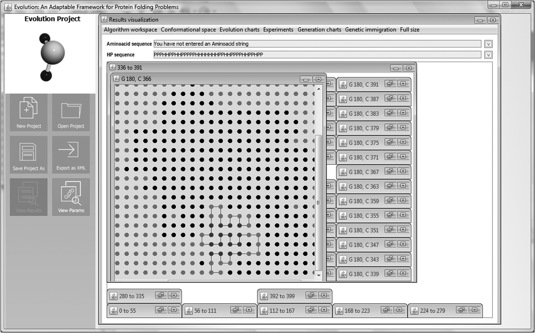
Arrangement of the experiment number 7 of the 36-HP sequence during the optimal conformation on the cluster grain with ξ = 11.70. The H and P residues are labeled in dark gray and light gray, respectively, whereas the cluster grain and vacuum space are marked in black and gray, respectively. This optimal conformation belongs to the generation 180.

4.2. Evaluating the effects of the homogeneous and inhomogeneous space on HP sequence folding

Until now, we have only evaluated the step-by-step folding of HP S1 on an inhomogeneous space in 10 experiments. To compare the behavior of the sequence in both environments, the same sequence was also analyzed in a homogenous space in 10 experiments; S2 and S3 were also analyzed in this way. The results obtained for these experiments are shown in Figure 17, where it is possible to observe the behavior of the optimal (ground energy state) and suboptimal fitness for each experiment on each sequence. The main results of this figure are described later.

FIG. 17.

Behavior in the independent experiments during 2D HP sequences folding on a homogeneous network and on a correlated network with ξ = 11.70 and d_f = 1.764.

4.2.1. Sequence S1: P₃H₂P₂H₂P₅H₇P₂H₂P₄H₂P₂HP₂; length: 36; score: −14

Figure 17a shows that when the 36-HP sequence (S1) was folded in a homogeneous network, the global minimum energy was not reached, whereas folding of the sequence in the inhomogeneous medium provided two times the optimum value of −14 (experiments 3 and 7; Table 2).

4.2.2. Sequence S2: P₂H(P₂H₂)₂P₅H₁₀P₆(H₂P₂)₂HP₂H₅; length: 48; score: −23

The minimum energy state was never found for S2 while folding in the homogeneous space (Fig. 17b). In this set of experiments, we found that the highest and final scores corresponded to −21. However, the evolution of the folding process in experiment 10 (black line, Fig. 17b) reaches maximal and final scores of −23 as previously reported (König and Dandekar, 1999; Liang and Wong, 2001; Thachuk et al., 2007). Moreover, a suboptimal structure with a final score of −22 was achieved in experiment 5, and six experiments had a final score of −21 when we used an inhomogeneous space. Hence, there are more experiments with better energy states in the inhomogeneous space than the homogeneous one.

4.2.3. Sequence S3: P₂H₃PH₈P₃H₁₀PHP₃H₁₂P₄H₅PH₂PHP; length: 60; score: −36

Figure 17c illustrates the folded 60-HP conformation for S3 in both homogenous and inhomogenous spaces. The best fitness was found to be −34 (experiment 3) for experiments performed in the correlated network, and −31 (experiment 8) in the homogeneous network. It is pertinent to mention that the worst value in the inhomogeneous space was −31, an −27 in the homogeneous space. Therefore, S3 folded into the inhomogeneous space better than in the homogeneous one in all 10 experiments. However, S3 did not reach the minimum energy state reported in the literature (−36). Here, we only performed 10 experiments to compare the effect exerted by the medium on the folding of the sequence. If the size of populations, generations, and/or number of experiments were increased, it may be possible to attain the optimal score; nevertheless, we allowed the same running and evaluation parameters for all three tested sequences. Figure 18 shows the suboptimal state of S3 on a cluster grain; it has a highly regular shape, where formation of the hydrophobic core (beads in dark gray) can be observed as a compact structure surrounded by polar residues (beads in light gray).

FIG. 18.

Arrangement of the experiment number 3 of the 60-HP sequence during the sub-optimal score (−34) on a cluster grain with ξ = 11.70. The colors labeled are the same as Figure 16. This optimal conformation belongs to the generation 100.

4.3. Insights in reaching the global energy minimum and the folded states in the simulation

Reaching the global energy minimum of a folded protein structure is not an easy task experimentally or computationally. Some reviews dealing with experimental techniques have a dramatically improved time resolution, thereby thoroughly contributing to the understanding of PF kinetics and mechanisms. These include optical triggering with nanosecond laser pulse techniques and improvements in the use of dynamic nuclear magnetic resonance methods, among others. Through these techniques it was possible to determine the fastest folding kinetics to be approximately ≥10³/s (Eaton et al., 2000). Furthermore, in the modeling sciences, statistical mechanical models have been extremely useful in interpreting experimental results through the dynamics of the studied systems, explaining the kinetics of structure formation, as well as calculating the folding rates required to reach the native 3D structure (Eaton et al., 2000). Other strategies were not intended to reproduce experimental evidence, but to obtain the minimum energy of the folded structure, as in the current study; they employed the Metropolis Monte Carlo rules to reach the folded states of proteins. These rules were merely designed for convenience and a computationally fast approach to equilibrium (Zwanzig, 1997). These rules were not constructed with a theoretical basis; therefore, they should not be used to track kinetics. However, they do provide useful results from a structural point of view (Zwanzig, 1997). With these two examples in mind, the new strategy presented herein was not aimed at obtaining the complete kinetic parameters of the PF process, as in Monte Carlo techniques, but merely as an alternative heuristic strategy or artificial shortcut to reach or find the minimum energy of the folded states of a given peptidic chain, traduced to a simplistic HP sequence. Thus, the current approach was not intended to simulate the experimental pathways of folding, but to attain the best possible minimum energy conformation of the folded structure.

The only mimicking strategy used herein is that the GA technique allowed interaction with a given initial population size or sample conformation space in an analogous manner to those of parallel kinetic models stated by Schonbrun and Dill (2003). To further explain this issue, it is well known that when microscopic kinetic steps happen in series, the macroscopic flux is limited by the microscopic bottleneck rate of a single process. But in cases where parallel microscopic routes exist (or a sample space of conformations for comparison purposes), this kinetic flux is greater (because the bottleneck in such cases depends on the size of the initial population and not on a single conformation) than the flux observed for the kinetics in series, because a bunch of conformational processes occur at the same time (Schonbrun and Dill, 2003). In this simple example, the efficiency of the employed GA is explained, as well as the fastest way to obtain results. Analogously, if the initial population is big enough, this optimization should occur faster, because a bunch of conformational processes occur at the same time while just taking into account the computational task force to overcome the management of such big sample spaces. Therefore, there is a compromise between fast optimization and computational capacity in the threshold to handle the biggest possible sample spaces with good optimization results in these clever approaches.

4.4. Relationship between our computational results and already known experimental results on PF

From the physicochemical point of view, Kramers' theory has been a cornerstone not only to modeling but also to understanding PF kinetics. This is because the time scale is mainly driven by a friction coefficient, which can be mainly attributed to the viscosity of the surrounding medium where it is included in the molecular crowding (Zwanzig, 1997). For example, in a dynamic conformational study of myoglobin, Ansari et al. (1992) found that Kramers' theory fitted their observed results very accurately, and this occurred when solvent viscosity and internal friction were included in the model.

From the molecular point of view, by now there are several experimental examples of unfolded states of proteins being optimally folded by employment of molecular crowding agents. Moreover, not only has folding been found to be influenced by the addition of other molecules, but also protein structure, shape, conformational stability, binding of small molecules, enzymatic activity, protein–protein interactions, protein–nucleic acid interactions, and pathological aggregation (Ådén and Wittung-Stafshede, 2014; Kuznetsova et al., 2014). This is the case for ribonuclease A, which was used to investigate the effects of macromolecular crowding on macromolecular compactness and PF measured by circular dichroism spectroscopy, fluorescence correlation spectroscopy, and nuclear magnetic resonance spectroscopy in the presence of polyethylene glycol or Ficoll as independent crowding agents. Obtained results in these approaches have shown that compact conformations are favored by macromolecules in the presence of a high concentration of other macromolecules, demonstrating the importance of crowded environments for folding and stabilization of protein systems (Tokuriki et al., 2004) and modeled through a correlated network in the current study. In other reports, key observations were found regarding macromolecular crowding effects on protein stability, folding, and structure, including in vitro and in silico studies. According to Minton's predictions (Minton, 1981), these facts occur when the fraction of volumen occupied by globular macromolecules increases, including:

(a) Compact quasi-spherical macromolecular conformations become increasingly energetically favored over extended anisometric conformations.

(b) Self- and hetero-association processes are enhanced, particularly those leading to the formation of compact quasi-spherical aggregates.

(c) Depending on the details of the reaction mechanism, the rate of an enzyme-catalyzed reaction may monotonically decrease, go through a maximum, or exhibit more complex behavior.

In this line, many proteins (e.g., apoflavodoxin, surface lipoprotein E (VlsE), cytochrome c, and ribosomal protein S16) became more thermodynamically stable and, unexpectedly for apoflavodoxin and VlsE, both folded states changed their secondary structure content and, for VlsE, overall shape in the presence of macromolecular crowding. For apoflavodoxin and cytochrome c, excluded volume effects due to crowding made folding energy landscapes smoother than in buffer media and, therefore, resulted in a lower probability of misfolding (Christiansen et al., 2013). All these studies clearly show that molecular crowding is a very important variable, mainly for smoothing the kinetic landscapes of folding, but a difficult one to include to understand the structure and function of (bio)molecules. For these reasons, we included a mimetic crowding environment as a simple correlated network in the 2D square lattice that provides better folding results compared with the noncorrelated or homogeneous space.

5. Conclusions

In the current work, we analyzed three HP sequences folded in two types of spaces: (1) homogeneous and (2) inhomogeneous. Analysis of the folding of S1 in the correlated network was explained step by step by using our upgraded Evolution bioinformatics platform. The correlated networks were built from the DSBM, which is fairly simple and capable of describing random media with different topological structures, mimicking inhomogeneous media, and folding the HP sequences by GA. Our preliminary results showed that the correlated network was more efficient than the homogeneous network at correctly folding the 2D HP sequences. When the sequences were folded in the homogeneous space, the chains had more degrees of freedom for determining the best energy state. Thus, in this space and condition, it was not possible to reach energy minima. However, when the sequences were folded in the inhomogeneous space on the cluster grain of a correlated network ξ = 11.70, we acheived a better conformation in all cases, with two sequences reaching previously published values and one obtaining a very good conformational approximation. In addition, the cluster grain energetically constrained the conformations (i.e., the correlated and fractal environment restricted the degrees of freedom of the conformation itself) as occurs in the intracellular medium. Therefore, our results demonstrated that the correlated network media (tracked as ξ) affects the folding of our HP sequences, ensuring that the intracellular environment plays a crucial role during the PF process.

Footnotes

Author Disclosure Statement

No competing financial interests exist.

References

Ådén

, and Wittung-Stafshede

2014. Folding of an unfolded protein by macromolecular crowding in vitro. Biochemistry. 53, 2271–2277.

Alas

S.J.

, and González-Pérez

P.P.

2016. Simulating the folding of HP-sequences with a minimalist model in an inhomogeneous medium. BioSystems. 142, 52–67.

Ansari

, Jones

C.M.

, Henry

E.R.

, et al. 1992. The role of solvent viscosity in the dynamics of protein conformational changes. Science. 256, 1796–1798.

Aon

M.A.

, and Cortassa

1994. On the fractal nature of cytoplasm. FEBS Lett. 334, 1–4.

Banga

J.R.

2008. Optimization in computational systems biology. BMC Syst. Biol. 2, 47.

Beltrán

H.I.

, Rojo-Domínguez

, Sánchez

M.E.

, et al. 2009. Exploring dimensionality, systemic mutations and number of contacts in simple HP ab-initio protein folding using a blackboard-based agent platform. Int. J. Inf. Commun. Eng., 5, 479–488.

Cervantes-Ojeda

, Sánchez-Gutiérrez

M.E.

, and González

P.P.

2010. Emerging traits in the application of an evolutionary algorithm to a scalable bioinformatics problem, 2082–2089. In Proceedings of the WCCI 2010 IEEE World Congress on Computational Intelligence (CCIB), Barcelona, Spain.

Christiansen

, Wang

, Cheung

M.S.

, et al. 2013. Effects of macromolecular crowding agents on protein folding in vitro and in silico. Biophys. Rev. 5, 137–145.

Cox

G.A.

, Mortimer-Jones

T.V.

, Taylor

R.P.

, et al. 2004. Development and optimization of a novel genetic algorithm for studying model protein folding. Theor. Chem. Acc. 112, 163–178.

10.

Dill

K.A.

1985. Theory for the folding and stability of globular-proteins. Biochemistry. 24, 1501–1509.

11.

Eaton

W.A.

, Muñoz

, Hagen

S.J.

, et al. 2000. Fast kinetics and mechanisms in protein folding. Annu. Rev. Biophys. Biomol. Struct. 29, 327–359.

12.

Ellis

R.J.

2001. Macromolecular crowding: An important but neglected aspect of the intracellular environment. Curr. Opin. Struct. Biol. 11, 114–119.

13.

Ellis

R.J.

, and Minton

A.P.

2003. Join the crowd. Nature. 425, 27–28.

14.

Goldberg

D.E.

1989. Genetic Algorithms in Search, Optimization, and Machine Learning. Addison-Wesley Professional, Boston, MA.

15.

González

P.P.

, Beltrán

H.I.

, Rojo-Domínguez , et al. 2009. Multi-agent systems applied in the modeling and simulation of biological problems: A case study in protein folding. World Acad. Sci. Eng. Technol. 58, 463–472.

16.

Gupta

, Manuch

, and Stacho

2005. Structure-approximating inverse protein folding problem in the 2D HP model. J. Comput. Biol. 12, 1328–1345.

17.

Homouz

, Perham

, Samiotakis

, et al. 2008. Crowded, cell-like environment induces shape changes in aspherical protein. Proc. Natl. Am. Sci. 105, 11754–11759.

18.

Hoque

, Chetty

, and Sattar

2009. Extended HP model for protein structure prediction. J. Comput. Biol. 16, 85–103.

19.

Hoshen

, and Kopelman

1976. Percolation and cluster distribution. I. Cluster multiple labeling technique and critical concentration algorithm. Phys. Rev. B. 14, 3438–3445.

20.

Huang

, Yang

, and He

2010. Protein folding simulations of 2D HP model by the genetic algorithm based on optimal secondary structures. Comp. Biol. Chem. 34, 137–142.

21.

Kaipio

J.P.

, and Somersalo

2004. Statistical and Computational Inverse Problems: Applied Mathematical Sciences. 160, 2005 edition, Springer, New York, NY.

22.

Kitano

2002. Computational systems biology. Nature. 420, 206–210.

23.

König

, and Dandekar

1999. Improving genetic algorithms for protein folding simulations by systematic crossover. BioSystems. 50, 17–25.

24.

Kurakin

2011. The self-organizing fractal theory as a universal discovery method: The phenomenon of life. Theor. Biol. Med. Model. 8, 1–66.

25.

Kuznetsova

I.M.

, Turoverov

K.K.

, and Uversky

V.N.

2014. What macromolecular crowding can do to a protein. Int. J. Mol. Sci., 15, 23090–23140.

26.

Levinthal

1968. Are there pathways for protein folding?. J. Chim. Phys. 65, 44–45.

27.

Liang

, and Wong

W. H.

2001. Evolutionary Monte Carlo for protein folding simulations. J. Chem. Phys. 115, 3374–3380.

28.

Lodhi

H.M.

, and Muggleton

S.H.

2010. Elements of Computational Systems Biology. Wiley & Sons, Inc., Hoboken, NJ.

29.

Luby-Phelps

2000. Cytoarchitecture and physical properties of cytoplasm: Volume, viscosity, diffusion, intracellular surface area. Int. Rev. Cytol. 192, 189–221.

30.

Minton

A.P.

1981. Excluded volume as a determinant of macromolecular structure and reactivity. Biopolymers, 20, 2093–2120.

31.

Minton

A.P.

2001. The influence of macromolecular crowding and macromolecular confinement on biochemical reactions in physiological media. J. Biol. Chem. 276, 10577–10580.

32.

Mitchell

1999. An Introduction to Genetic Algorithms (Complex Adaptive Systems). The MIT Press, Cambridge, MA.

33.

Mittal

, and Singh

L.R.

2014. Macromolecular crowding induces holo-lactalbumin aggregation by converting to its apo form. PLoS One, 9, e114029, 1–20.

34.

Munishkina

L.A.

, Ahmad

, Fink

A.L.

, et al. 2008. Guiding protein aggregation with macromolecular crowding. Biochemistry. 47, 8993–9006.

35.

Omenn

G.S.

2006. Grand challenges and great opportunities in science, technology, and public policy. Science. 314, 1696–1704.

36.

Pattanasiri

, Li

Y.W.

, Landau

D.P.

, et al. 2013. Thermodynamics and structural properties of a confined HP protein determined by Wang-Landau simulation. J. Phys. Conf. Ser., 454, 012071.

37.

Patton

A.L.

III , Punch

W.F.

, and Goodman

E.D.

1995. A standard GA approach to native protein conformation prediction, 574–581. In Proceedings of the Sixth International Conference on Genetic Algorithms. San Mateo, CA.

38.

Ping

, Yuan

J.M.

, Vallieres

, et al. 2003. Effects of confinement on protein folding and protein stability. J. Chem. Phys. 118, 8042–8048.

39.

Schonbrun

, and Dill

K.A.

2003. Fast protein folding kinetics. Proc. Natl. Acad. Sci., 100, 12678–12682.

40.

Shmygelska

, and Hoos

H.H.

2005. An ant colony optimisation algorithm for the 2D and 3D hydrophobic polar protein folding problem. BMC Bioinformatics, 6, 30.

41.

Thachuk

, Shmygelska

, and Hoos

H.H.

2007. A replica exchange Monte Carlo algorithm for protein folding in the HP model. BMC Bioinformatics, 8, 342.

42.

Tokuriki

, Kinjo

, Negi

, et al. 2004. Protein folding the effects of macromolecular crowding. Protein Sci. 13, 125–133.

43.

Unger

, and Moult

1993. Genetic algorithms for protein folding simulation. J. Mol. Biol. 231, 75–81.

44.

van den Berg

, Ellis

R.J.

, and Dobson

C.M.

1999. Effects of macromolecular crowding on protein folding and aggregation. EMBO J. 18, 6927–6933.

45.

Vasilescu

, Olteanu. M., Flondor

, et al. 2013. Fractal-like kinetics of intracellular enzymatic reactions: A chemical framework of endotoxin tolerance and a possible non-specific contribution of macromolecular crowding to cross-tolerance. Theor. Biol. Med. Model., 10, 1–19.

46.

Vogel

C.R.

2002. Computational Methods for Inverse Problems. Computational methods for inverse problems (SIAM), Philadelphia, PA.

47.

Zwanzig

1997. Two-state models of protein folding kinetics. Proc. Natl. Acad. Sci., 94, 148–150.

A Computational Approach to Studying Protein Folding Problems Considering the Crucial Role of the Intracellular Environment

Abstract

Abstract

1. Introduction

2. Modeling of Inhomogeneous Space Through DSBM

3. The Evolution Bioinformatics Tool

3.1. Algorithmic and representational aspects in Evolution

3.1.1. The 2D/3D HP representation

3.1.2. Search and optimization of 2D/3D structures

3.1.3. Optimization functions

3.1.4. Types of conformational spaces, conformations, and connectivity

3.1.5. The GA

3.2. Evolution workflow

3.3. Application accessibility

4. Results and Discussion

4.1. Step-by-step HP sequence folding in an inhomogeneous space of a correlated network type

4.2. Evaluating the effects of the homogeneous and inhomogeneous space on HP sequence folding

4.2.1. Sequence S1: P3H2P2H2P5H7P2H2P4H2P2HP2; length: 36; score: −14

4.2.2. Sequence S2: P2H(P2H2)2P5H10P6(H2P2)2HP2H5; length: 48; score: −23

4.2.3. Sequence S3: P2H3PH8P3H10PHP3H12P4H5PH2PHP; length: 60; score: −36

4.3. Insights in reaching the global energy minimum and the folded states in the simulation

4.4. Relationship between our computational results and already known experimental results on PF

5. Conclusions

Footnotes

Author Disclosure Statement

References

4.2.1. Sequence S1: P₃H₂P₂H₂P₅H₇P₂H₂P₄H₂P₂HP₂; length: 36; score: −14

4.2.2. Sequence S2: P₂H(P₂H₂)₂P₅H₁₀P₆(H₂P₂)₂HP₂H₅; length: 48; score: −23

4.2.3. Sequence S3: P₂H₃PH₈P₃H₁₀PHP₃H₁₂P₄H₅PH₂PHP; length: 60; score: −36