Machine Learning Approaches for Predicting Protein Complex Similarity

Abstract

Discriminating native-like structures from false positives with high accuracy is one of the biggest challenges in protein–protein docking. While there is an agreement on the existence of a relationship between various favorable intermolecular interactions (e.g., Van der Waals, electrostatic, and desolvation forces) and the similarity of a conformation to its native structure, the precise nature of this relationship is not known. Existing protein–protein docking methods typically formulate this relationship as a weighted sum of selected terms and calibrate their weights by using a training set to evaluate and rank candidate complexes. Despite improvements in the predictive power of recent docking methods, producing a large number of false positives by even state-of-the-art methods often leads to failure in predicting the correct binding of many complexes. With the aid of machine learning methods, we tested several approaches that not only rank candidate structures relative to each other but also predict how similar each candidate is to the native conformation. We trained a two-layer neural network, a multilayer neural network, and a network of Restricted Boltzmann Machines against extensive data sets of unbound complexes generated by RosettaDock and PyDock. We validated these methods with a set of refinement candidate structures. We were able to predict the root mean squared deviations (RMSDs) of protein complexes with a very small, often less than 1.5 Å, error margin when trained with structures that have RMSD values of up to 7 Å. In our most recent experiments with the protein samples having RMSD values up to 27 Å, the average prediction error was still relatively small, attesting to the potential of our approach in predicting the correct binding of protein–protein complexes.

1. Introduction

Proteins play a major role in nearly any vital biological function (Gray, 2006; Lesk, 2008). Proteins often bind to other proteins to form complexes (Goodsell and Olson, 2000). To understand the important roles proteins play, we must have good understanding of their structure and function (Gray, 2006; Kastritis and Bonvin, 2010; Moal et al., 2013).

Computational docking methods aim to compute the correct bound form of two or more molecules. This is highly challenging because even for rigid body docking, the solution space spans the three translational and three rotational degrees of freedom for the other protein, and it grows exponentially with the size of the input proteins (Cherfils and Janin, 1993; Moreira et al., 2010). Most docking algorithms apply a geometric search for the correctly bound complex, followed by a ranking/scoring stage where a scoring function aims to distinguish native-like candidates from false positives. Several modern docking algorithms are successful in predicting the correctly bound complex of their input proteins, but many of the highest ranking docking candidates are still false positives (Halperin et al., 2002; Janin, 2010).

It is generally agreed that there is a relationship between various scoring terms (e.g., Van der Waals [VdW], electrostatic, and desolvation forces) and the similarity of a docking output complex to its native structure (Moal et al., 2013). However, the exact form of this relationship is unknown. Therefore, docking algorithms often formulate this relationship as a weighted sum of selected energetic, biochemical, or geometric terms and adjust their weights against a training set (Moal et al., 2013). However, the general inaccuracy of the rankings may suggest that this relationship may be more complex than a weighted sum (Kastritis and Bonvin, 2010). For this reason, many docking algorithms provide an additional, sometimes optional, refinement stage.

In this work, we describe three methods to predict the RMSD of a set of docking refinement candidates with respect to their native conformation. We train the models using different data sets with the goal of determining the training data set that gives the highest prediction power. By building three models to predict the RMSD of a given structure, we provide the experimental setting for comparing the performance of these models. These experiments can be used as a guiding tool for building the right data set and designing the best model in the studies that rely on selecting the best docking refinement candidates.

1.1. Scoring functions for protein–protein docking

Over the past 20 years, several scoring functions have been developed for ranking putative docked complexes. These functions combine geometric complementarity with physicochemical interactions (Halperin et al., 2002). Most scoring functions use a combination of VdW energy, electrostatic interactions, and desolvation terms (Dominguez et al., 2003; Comeau et al., 2004; Cheng et al., 2007; Pierce and Weng, 2007; Lyskov and Gray, 2008; Vries and Zacharias, 2013). The combination and weighing of the terms vary among methods. A recent docking refinement method (Akbal-Delibas et al., 2012; Akbal-Delibas and Haspel, 2013) uses a scoring function, including an evolutionary traces (ET) term (Mihalek et al., 2006; Wilkins et al., 2012), in addition to the VdW and electrostatic components.

While it is known that proteins often change their conformations upon binding, modeling flexibility is challenging due to the additional computational cost to an already difficult problem. Flexible docking methods use normal mode analysis (Li et al., 2010) and side-chain flexibility combined with soft rigid body optimization (Lyskov and Gray, 2008; Mashiach et al., 2008). Despite recent development in scoring functions, predicting the correct binding conformation is still a largely unsolved problem. A recent large-scale benchmarking of current docking methods revealed that most current physics-based scoring functions still fail to accurately predict the binding affinity of complexes (Kastritis and Bonvin, 2010).

1.2. Neural networks

Neural networks are widely used to approximate complex functions. In previous work (Akbal-Delibas et al., 2014, 2015b), we used a backpropagation network (Rumelhart et al., 1986; Werbos, 1990; Mehrotra et al., 1997) to formulate the relationship between a wide set of scoring function terms and RMSD of a docked structure. The tool, denoted AccuRMSD, not only ranks the decoys relative to each other but also indicates how similar each decoy is to the native conformation.

Recently, more sophisticated types of networks, called deep-learning networks, have shown great success in the domain of image processing, speech recognition, and bioinformatics. In deep architectures, multiple layers of nonlinear mappings are stacked on top of one another to better capture the nonlinearities in the representation of training data. These multiple hidden layers build a hierarchy that transforms the raw input to a feature space that is often initially unobserved. The rapid advances in computing hardware as well as availability of vast volumes of data at low cost have enabled the efficient training of deep networks. We used deep learning in the past to aid in docking refinement (Akbal-Delibas et al., 2015a, 2016). In this work, we have used a multilayer neural network (MLNN) as well as a network of restricted Boltzmann machines (RBMs) (Yu and Deng, 2011).

2. Methods

2.1. Training data sets

The first set of data sets, used in the conference version of this article (Farhoodi et al., 2015), includes 41 protein structures with RMSD values that range between 0 and 7 Å and divided into training and testing sets of 35 and 6 proteins, respectively. The second set of data sets was added to this extended version to test a more diverse set of putative complexes. It includes 54 proteins where the RMSD values span a much wider range, between 0 and 27 Å. We have divided these into training and testing data sets of 48 and 6 proteins, respectively. Table 1 provides information of all the data sets used in this article. In what follows, we provide more details about the data sets.

Table 1.

Training and Testing Data sets Statistics Summary: Minimum, Mean, Maximum, and Standard Deviation of the RMSD Values of the Samples in Each Data set and the Methods Used to Generate the Samples

Dataset name	Min	Mean	SD	Max	Method
Docked structures	1.03	2.51	0.84	6.67	Rosetta
Ref. candidates 1	1.06	4.79	2.67	6.99	Rosetta
Combined structures	1.03	3.60	2.31	6.99	Rosetta
Test ref. candidates 1	0.92	3.82	1.74	6.99	Rosetta
Ref. candidates 2	0.92	4.49	2.30	24.46	Rosetta
Ref. candidates 3	0.82	8.38	3.56	26.88	pyDock
Test ref. candidates 2	0.92	4.3	2.13	15.16	Rosetta
Test ref. candidates 3	1.26	9.01	4.08	22.55	pyDock

Ref, refinement.

2.1.1. Protein structures with limited RMSD range

We initially trained our models with three extensive data sets that included the following 35 unbound dimer proteins listed in the unbound Protein–Protein Docking Benchmark 4.0 (Hwang et al., 2010): 1B6C, 1EFN, 1EWY, 1FFW, 1GL1, 1GLA, 1GPW, 1GXD, 1H9D, 1US7, 1J2J, 1JTG, 1OC0, 1OYV, 1PVH, 1S1Q, 1T6B, 1XD3, 1YVB, 1Z0K, 1Z5Y, 1ZHH, 1ZHI, 2AST, 2AJF, 2B42, 2FJU, 2HLE, 2HQS, 2J0T, 2O8 V, 2OOB, 2VDB, 3DSS, and 4CPA. We focused on the dimers from the rigid body category in this benchmark and selected the proteins for which the corresponding ET files were available in the ET Server (Mihalek et al., 2006). Our methods were initially designed to accurately discriminate docking refinement candidates generated from putative docked protein complexes. Therefore, in addition to the docked structures, we generated a set of refinement candidates. We grouped these samples into three data sets based on the method used to generate the corresponding protein structures:

• Docked structures data set: For each protein, we produced 1000 docked structures by RosettaDock (Lyskov and Gray, 2008). We used the coarse grained module (without refinement), followed by 500 minimization steps using NAMD (Phillips et al., 2005) to resolve clashes without significantly changing the structures. We then analyzed the interfaces of each structure and calculated the values of the network features. This data set consists of 35,000 samples.

• Refinement candidates data set: For each protein, we generated 1000 refinement candidates from coarsely docked complexes by applying small rigid body rotations around an arbitrary axis as described in Akbal-Delibas et al., 2015a. This initially resulted in 35,000 refinement candidates, of which ∼6000 were discarded due to high RMSD values (above 7Å), with the aim of obtaining an approximately normal distribution.

• Docked and refinement structures data set: We combined the samples in the docked structures data set and the refinement candidates data set. This data set consisted of ∼64,000 samples.

Our motivation of building these data sets was to investigate how adding the refinement candidates to the docking training set affects the accuracy of the model. Figure 1a–c depicts the RMSD (Å) distribution of samples in these data sets.

FIG. 1.

RMSD (Å) distribution of (a) the docked structures training data set, (b) the refinement candidates training data set, (c) the docked structures and refinement candidates training data set, and (d) the refinement candidates test set. The RMSD is with respect to the native PDB structure.

2.1.2. Protein structures with higher RMSD range

To evaluate the accuracy of methods in cases where structures have higher RMSD values, we generated two new training data sets of the following 48 proteins: 2A5T, 3D5S, 1S1Q, 1Z5Y, 2AJF, 2GAF, 1GLA, 1GPW, 1XD3, 2A1A, 1FFW, 1JTD, 1YVB, 2GTP, 1EWY, 3A4S, 1J2J, 2J0T, 1T6B, 1US7, 1OC0, 1ZHI, 1OYV, 1H9D, 2I25, 2VDB, 4M76, 1ZHH, 2HLE, 1EFN, 1B6C, 2OOB, 2O8V, 4CPA, 1Z0K, 1PVH, 4H03, 3BIW, 3VLB, 1GL1, 2YVJ, 1GXD, 2B42, 3K75, 3PC8, 2HQS, 1JTG, and 2FJU. This set includes the proteins in the previous data sets and 13 extra proteins that we have newly added to the collection after the release of the Protein–Protein benchmark v.5 (Vreven et al., 2015). Also, in addition to RosettaDock, we have used pyDock (Jiménez-García et al., 2013) to generate samples. Based on the method used to generate these data sets, we have divided the samples into two classes of structures:

• RosettaDock structures: For each protein named above, we have generated 1000 refinement candidates from coarsely docked protein structures produced by RosettaDock, which resulted in 48,000 samples. The RMSD values of the structures range between 0.92 and 24.46 Å.

• pyDock structures: Similarly, we generated 1000 refinement candidates from complexes produced by pyDock (Jiménez-García et al., 2013) without any distance restraints. These samples have RMSD values that vary between 0.82 and 26.88 Å.

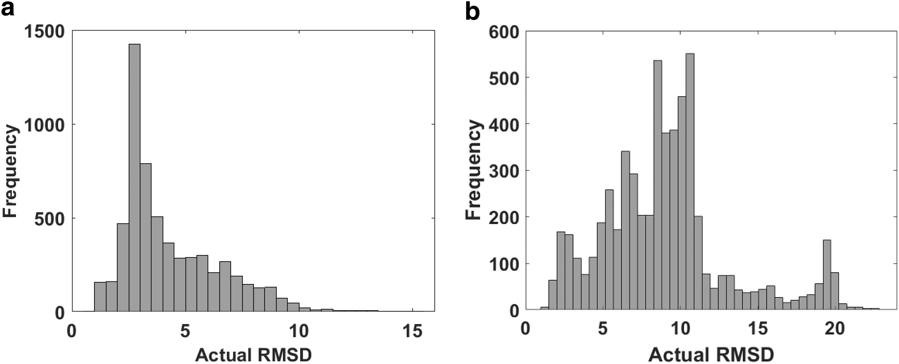
The distribution of RMSD values for these data sets is shown in Figure 2, and more statistics are presented in Table 1.

FIG. 2.

RMSD (Å) distribution of (a) training data set generated by RosettaDock and (b) training data set generated by pyDock.

2.2. Test data sets

The models were tested on three data sets of refinement candidates produced from coarsely docked protein complexes generated by RosettaDock and pyDock. The sets include six proteins named 1R0R, 2A9K, 2AYO, 2G77, 2SNI, and 7CEI. For each protein, we selected five docked complexes, and for each of these complexes, 200 refinement candidates were generated by applying small-scale rigid body rotations resulting in a total of 6000 samples in each data set. The test data sets are divided into three classes based on the method that was used to generate them and the samples' RMSD range:

• Refinement candidates 1: generated by RosettaDock, with RMSD range between 0.92 and 7 Å. Figure 1d displays the RMSD distribution of these structures.

• Refinement candidates 2: generated by RosettaDock, with RMSD between 0.92 and 15.16 Å. The RMSD distribution is shown in Figure 3a.

• Refinement candidates 3: generated by pyDock program, with RMSD between 1.26 and 16.40 Å. The RMSD distribution is shown in Figure 3b.

FIG. 3.

RMSD (Å) distribution of (a) test data set generated by RosettaDock and (b) test data set generated by PyDock.

Table 1 shows the summary of the statistics for all training and test data sets.

2.3. Features

Our methods approximate the relationship between 16 different features and the RMSD of a protein complex with respect to its native structure. The majority of these features are used as scoring function terms by a number of docking and refinement methods and were used by us in the past (Akbal-Delibas et al., 2012).

• VdW: Computed for interface atoms (atoms within at most 6 Å to the adjacent chain atoms).

• Electrostatic: Computed for interface atoms.

• Interface conserved atom ratio: The ratio of the evolutionarily conserved interface atoms to the total interface size.

• Protein Category: 1: Antibody Antigen, 2: Antigen-Bound Antibody, 3: Enzyme Inhibitor, 4: Enzyme complex with a regulatory or accessory chain, 5: Enzyme Substrate, 6: G-protein containing, 7: Receptor containing, 8: miscellaneous. The categories are taken from the Protein–Protein Docking Benchmark v.5 (Vreven et al., 2015).

• The ratios of interface atoms belonging to residue types to the total interface size: Hydrophobic (A, C, G, I, L, M, P, V); Positively Charged (H, K, R); Negatively Charged (D, E); Polar (N, Q, S, T); and Aromatic (F, H, W, Y).

2.4. Prediction methods

We developed three models to predict the RMSD of the tested candidates. We now describe the configuration of each model.

2.4.1. Two-layer neural network

In Akbal-Delibas et al., 2014, 2015a,b, we introduced a neural network trained using the backpropagation algorithm. In this study, we use the same network with 16 features described above. The network has 16 input neurons, which receive input data, including 16 features that characterize a protein structure. Eight of these features consist of continuous values and were initially normalized to the range of \documentclass{aastex}\usepackage{amsbsy}\usepackage{amsfonts}\usepackage{amssymb}\usepackage{bm}\usepackage{mathrsfs}\usepackage{pifont}\usepackage{stmaryrd}\usepackage{textcomp}\usepackage{portland, xspace}\usepackage{amsmath, amsxtra}\pagestyle{empty}\DeclareMathSizes{10}{9}{7}{6}\begin{document} $$[ 0..1 ]$$ \end{document} before being fed to their corresponding neurons. The remaining eight features, which are used to represent the eight different protein categories, are fed into binary neurons since they take binary values only. Our experiments showed that 100 hidden-layer neurons led to the best prediction results. The output layer consists of one neuron that generates the predicted RMSD value. This output value is in the range of \documentclass{aastex}\usepackage{amsbsy}\usepackage{amsfonts}\usepackage{amssymb}\usepackage{bm}\usepackage{mathrsfs}\usepackage{pifont}\usepackage{stmaryrd}\usepackage{textcomp}\usepackage{portland, xspace}\usepackage{amsmath, amsxtra}\pagestyle{empty}\DeclareMathSizes{10}{9}{7}{6}\begin{document} $$[ 0..1 ]$$ \end{document} and is rescaled to represent the final predicted RMSD value. We trained this network for 300 epochs, where no further significant improvement was observed.

2.4.2. Multilayer neural network

This model has one input layer, three hidden layers, and one output layer. For comparison purposes, this network uses the same 16 input neurons to receive the input data. After parameter tuning, the network had 50 neurons in the first hidden layer and 70 and 100 neurons in the next two hidden layers. Similarly, the output layer consisted of one neuron that produces the predicted RMSD value. This network was also trained 300 epochs.

2.4.3. RBMs network

This network consists of three layers. The input layer is similar to the input layers of the two previous models. The hidden layer, which is fully connected to the input layer, includes 20 RBMs (Yu and Deng, 2011), and finally, the output layer consists of one output neuron. The RBMs were trained in an unsupervised manner by utilizing the feature values only, using a contrastive divergence (Hinton, 2012) algorithm and then weights between RMB layer and output layer were updated using the backpropagation learning method.

3. Results and Discussion

We conducted two set of experiments with our two data set collections of different RMSD ranges. We divide each subsection into an experiment with refinement candidates and cross-validation.

3.1. Experiments with data sets of smaller RMSD range

For the first set of experiments, we used the smaller data sets with RMSD ranges limited to a maximum value of 7 Å. First, we describe our prediction results after training the models with our data sets of smaller RMSD range. We then present our model comparison results after conducting 10-fold cross-validation.

3.1.1. Experiments with refinement candidates

First, we trained the models with the data set of RosettaDock docked structures. Then, we tested our test set of 6000 refinement candidates for six different proteins. We compared the predicted RMSD and the actual RMSD values through the root-mean-square (RMS) of the error made by the models. The Pearson correlation coefficients of the predicted and actual RMSD values and the error are listed in Table 2. The smallest prediction error was achieved by the MLNN and was 1.45 Å. The two-layer neural network (TLNN) performed slightly worse with 1.48 Å prediction error. In addition, the Pearson correlation coefficient between the predicted and actual RMSD values predicted by MLNN was higher (0.41). Next, we used the data set of refinement candidates for training. The error and correlation coefficients are listed in Table 3. As shown in the table, the prediction accuracy of the TLNN and MLNN deteriorated, while the restricted Boltzmann machine network (RBMN) showed a smaller error compared to the case where it was trained with the docked structures. Finally, we trained the models using the data set with both docked structures and refinement candidates. The results are presented in Table 4. Again, the lowest error (1.3 Å) was obtained using the MLNN. The accuracy of TLNN and RBMN was worse than the previous experiment. Here is the summary of our observations with respect to the training data set impact on the prediction accuracy of the models:

Table 2.

Pearson Correlation Coefficient and Prediction Error for the RMSD of Refinement Candidate Test Cases of Six Proteins (1000 Samples for Each Protein with RMSD Range of 0.92–6.99 Å) with Respect to Their Native Structure for the Three methods Trained on the Docked Structures Data set

PDB ID	TLNN correlation	TLNN error (Å)	MLNN correlation	MLNN error (Å)	RBMN correlation	RBMN error (Å)
1R0R	0.66	1.28	0.46	1.17	0.57	1.19
2A9K	0.18	1.87	0.45	1.54	0.50	1.90
2AYO	0.01	2.14	0.43	2.07	0.18	2.48
2G77	0.66	1.98	0.54	1.84	0.30	2.21
2SNI	0.34	0.44	0.41	0.54	0.25	0.80
7CEI	0.33	1.17	0.18	1.54	0.43	1.23
Overall	0.36	1.48	0.41	1.45	0.37	1.63

MLNN, multilayer neural network; RBMN, restricted Boltzmann machine network; PDB, protein data bank; RMSD, root mean squared deviation; TLNN, two-layer neural network.

Table 3.

PDB ID	TLNN correlation	TLNN error (Å)	MLNN correlation	MLNN error (Å)	RBMN correlation	RBMN error (Å)
1R0R	0.68	1.68	0.59	2.1	0.56	1.77
2A9K	0.05	2.70	0.03	1.35	0.08	1.10
2AYO	0.55	1.69	0.26	1.71	0.58	1.39
2G77	0.15	2.29	0.04	1.44	0.01	1.44
2SNI	0.51	0.99	0.11	1.9	0.34	1.05
7CEI	0.77	0.94	0.63	0.95	0.82	1.01
Overall	0.45	1.72	0.28	1.58	0.40	1.29

Table 4.

PDB ID	TLNN correlation	TLNN error (Å)	MLNN correlation	MLNN error (Å)	RBMN correlation	RBMN error (Å)
1R0R	0.56	1.52	0.53	1.74	0.65	0.96
2A9K	0.55	2.02	0.33	1.30	0.30	2.30
2AYO	0.13	2.28	0.07	1.60	0.49	1.73
2G77	0.63	2.90	0.58	0.97	0.26	1.94
2SNI	0.18	1.83	0.11	1.33	0.48	0.57
7CEI	0.75	1.33	0.58	1.05	0.83	1.52
Overall	0.47	1.98	0.37	1.33	0.50	1.50

• The TLNN performed best when trained with the data set of only docked structures. Its prediction error increased by 33% and 16% when the refinement candidates data set and the combined data set, respectively, were used for the training.

• The MLNN showed the lowest prediction error when trained using both docked structures and refinement candidates. The prediction error in this case was 18% lower than the case where it was trained using the refinement candidates data set. Furthermore, we observed a 9% increase in error, when we trained this model using docked structures only.

• The RBMN achieved the lowest error with the refinement candidates training data set.

The correlation coefficients and the prediction errors vary significantly from one protein to another. This is mainly due to the considerable diversity in the feature values and RMSD distributions of the test proteins. Furthermore, it indicates that each of the models was able to capture certain characteristics in the existing relation among the features and RMSD values of the test complexes and suggests that the prediction accuracy of the models can be improved by increasing the diversity among the training samples.

3.1.2. Model comparison by cross-validation

To analyze the performance of the models, we conducted a set of 10-fold cross-validation experiments. We randomly divided the data sets into two partitions for training and testing. The training consisted of 90% of the samples that were randomly selected and the remaining samples were used for testing. The average prediction errors of the models trained using the data sets are listed in Table 5. The cross-validation results show that the MLNN is outperforming the other two models in all the cases.

Table 5.

Ten-Fold Cross-Validation Average Error of the Models, Trained Using Three Data sets with Smaller RMSD Range

Model data set	Average error
TLNN-Docked	0.24
MLNN-Docked	0.17
RBMN-Docked	0.44
TLNN-Refined	0.91
MLNN-Refined	0.87
RBMN-Refined	1.27
TLNN-Combined	0.75
MLNN-Combined	0.47
RBMN-Combined	1.16

The best result in each category is shown in bold font.

Combined, docked and refinement structures data set; Docked, docked structures data set; Refined, refinement candidates data set.

3.2. Experiments with data sets of higher RMSD range

For the second set of experiments, we used our newer data sets with higher RMSD ranges of up to 27 Å. We present the results in two parts as before.

3.2.1. Experiments with refinement candidates

We trained the models with the data set that included refinement candidate structures produced by RosettaDock. Then, we tested the refinement candidates produced by RosettaDock. We compared the predicted and the actual RMSD values by calculating the RMS of the error made by the models. The Pearson correlation coefficients of the predicted and actual RMSD values and error are listed in Table 6. The smallest average error, 2.21 Å, and highest correlation coefficient (0.54) were achieved by the MLNN. The TLNN and RBMN performed very close to each other, being slightly worse than MLNN with 2.30 and 2.29 Å RMS errors, respectively. RBMN had a higher correlation coefficient on average.

Table 6.

Pearson Correlation Coefficient and Prediction Error for the RMSD of Refinement Candidate Test Cases of Six Proteins (1000 Samples for Each Protein with RMSD Range of 0.92–15.16 Å) with Respect to Their Native Structure for the Three Methods Trained on the Refined Structures Generated by RosettaDock

PDB ID	TLNN correlation	TLNN error (Å)	MLNN correlation	MLNN error (Å)	RBMN correlation	RBMN error (Å)
1R0R	0.67	2.59	0.71	2.21	0.65	2.69
2A9K	0.02	3.91	0.14	3.70	0.16	2.67
2AYO	0.61	2.21	0.61	2.42	0.60	2.40
2G77	0.04	1.64	0.44	1.60	0.64	1.19
2SNI	0.43	2.14	0.47	1.93	0.44	2.36
7CEI	0.82	1.29	0.85	1.41	0.41	2.45
Overall	0.43	2.30	0.54	2.21	0.50	2.29

Next, we used the data set of refinement candidates generated by pyDock for training. The results are listed in Table 7. The prediction accuracy of MLNN was the highest among the models with an average error of 2.84 Å and correlation coefficient of 0.43. The TLNN performed slightly worse with 2.88 Å average error and the RBMN performed the worst with 3.34 Å average prediction error. Generally, the errors of the models trained by pyDock complexes were larger and the correlation coefficients were lower compared to the models trained with samples generated by RosettaDock. We attribute this to having considerably more samples with lower RMSD values in the data sets generated by RosettaDock, while the complexes obtained by pyDock had a much wider range of RMSD values.

Table 7.

Pearson Correlation Coefficient and Prediction Error for the RMSD of Refinement Candidate Test Cases of Six Proteins (1000 Samples for Each Protein with RMSD Range of 1.26–22.55 Å) with Respect to Their Native Structure for the Three Methods Trained on the Refined Structures Generated by pyDock

PDB ID	TLNN correlation	TLNN error (Å)	MLNN correlation	MLNN error (Å)	RBMN correlation	RBMN error (Å)
1R0R	0.35	1.89	0.36	1.89	0.49	2.12
2A9K	0.23	2.03	0.27	2.03	0.18	2.19
2AYO	0.08	3.30	0.22	3.29	0.03	4.23
2G77	0.79	1.50	0.76	1.49	0.45	1.59
2SNI	0.76	5.03	0.78	4.79	0.65	3.95
7CEI	0.12	3.56	0.19	3.55	0.04	5.98
Overall	0.39	2.88	0.43	2.84	0.31	3.34

As seen, the MLNN outperforms the other two models independent of the training data set. As before, the correlation coefficients and the error of the models vary for different proteins. For instance, the TLNN and MLNN trained with the structures generated by RosettaDock showed the smallest error and highest correlation coefficient for 7CEI, while the RBMN had the lowest error in the experiments with the refinement candidates that belong to 2G77.

3.2.2. Model comparison by cross-validation

We conducted 10-fold cross-validation experiments with the two new data sets. We divided the samples into training and testing in an iterative manner, where no samples generated for a particular protein could fall in both training and testing sets. The errors and correlation coefficients of the models trained using RosettaDock data set are listed in Table 8. The results show that both the TLNN and MLNN are performing very closely with average errors of 1.91 and 1.92 Å, respectively, while the MLNN is showing slightly higher average correlation coefficients of 0.54. The cross-validation results with pyDock data set are shown in Table 9. The TLNN is showing the least error of 3.39 Å and highest correlation coefficients of 0.40. Once again the RBMN is the worst performing model.

Table 8.

Ten-Fold Cross-Validation Correlation Coefficient and Prediction Error for the RMSD Prediction of Refinement Candidates Generated by RosettaDock Using Three Methods

Fold	TLNN correlation	TLNN error (Å)	MLNN correlation	MLNN error (Å)	RBMN correlation	RBMN error (Å)
1	0.36	2.51	0.40	2.33	0.38	2.53
2	0.30	2.56	0.38	2.43	0.46	3.04
3	0.51	1.86	0.52	1.86	0.06	3.17
4	0.55	1.89	0.52	1.94	0.38	2.25
5	0.49	2.90	0.51	2.92	0.40	2.94
6	0.57	1.43	0.65	1.38	0.41	2.06
7	0.41	1.50	0.55	1.35	0.33	2.05
8	0.46	1.73	0.38	2.15	0.25	2.71
9	0.81	1.28	0.75	1.34	0.54	1.91
10	0.74	1.52	0.77	1.52	0.68	1.92
Average	0.52	1.91	0.54	1.92	0.39	2.46

Table 9.

Ten-Fold Cross-Validation Correlation Coefficient and Prediction Error for the RMSD Prediction of Refinement Candidates Generated by pyDock Using Three Methods

Fold	TLNN correlation	TLNN error (Å)	MLNN correlation	MLNN error (Å)	RBMN correlation	RBMN error (Å)
1	0.42	4.01	0.39	4.00	0.38	4.02
2	0.30	3.62	0.23	3.70	0.32	3.77
3	0.45	3.38	0.44	3.65	0.37	4.54
4	0.32	3.32	0.38	3.30	0.14	4.14
5	0.43	3.77	0.41	3.51	0.42	3.44
6	0.44	3.69	0.32	4.69	0.16	5.27
7	0.23	3.12	0.41	2.98	0.22	3.41
8	0.43	3.68	0.48	3.48	0.44	3.59
9	0.62	2.33	0.54	2.56	0.44	2.80
10	0.40	3.01	0.28	3.34	0.21	3.38
Average	0.40	3.39	0.39	3.52	0.31	3.84

4. Conclusions

We presented three models to accurately discriminate native-like structures during protein–protein docking and refinement: a TLNN, a MLNN, and a RBMN. These methods enabled us to approximate the nonlinear relationship between a set of selected features and a structure's similarity to its native conformation. We trained the models using several data sets with the primary motivation of investigating their predictive power for ranking of the refinement candidates. We tested the models with a group of refinement candidates generated from six other proteins. The RBMN produced the lowest error when trained with the refinement candidates data set of a smaller RMSD range. In the rest of the experiments, the MLNN outperformed the other models. Based on our experiments, MLNN is the method that shows the highest prediction accuracy in the majority of cases.

It is worth mentioning that despite training the models with samples of higher RMSD values, the average prediction error is still relatively small, which demonstrates the robustness of the methods to large RMSD changes. Furthermore, with the data sets of wide RMSD range, the correlation between the predicted and actual RMSD values was higher than the correlation obtained previously with data sets of lower RMSD ranges, being close to 0.5 on average and as high as 0.85 in some cases. This confirms that the models could benefit from a training data set with a diverse and wide range of samples. Future work includes the following directions. First, we plan to study other prediction methods. Second, we intend to boost our feature set by introducing new features that represent the protein complexes more accurately. Third, we are interested in testing the accuracy of these models on proteins under the medium and difficult categories of the Protein–Protein Docking Benchmark 5.0, as well as multimers. Finally, we will use these models as the ranking tool in a new method for refining coarsely docked protein complexes.

Footnotes

Acknowledgment

The research was funded in part by an NSF grant CCF-1421871 (N.H.).

Author Disclosure Statement

No competing financial interests exist.

References

Akbal-Delibas

, Farhoodi

, Pomplun

, et al. 2016. Accurate refinement of docked protein complexes using evolutionary information and deep learning. J. Bioinform. Comput. Biol., 14, 1642002.

Akbal-Delibas

, Hashmi

, Shehu

, et al. 2012. An evolutionary conservation-based method for refining and reranking protein complex structures. J. Bioinform. Comput. Biol. 10, 1242002.

Akbal-Delibas

, and Haspel

2013. A conservation and biophysics guided stochastic approach to refining docked multimeric proteins. BMC Struct. Biol. 13(Suppl 1), S7.

Akbal-Delibas

, Pomplun

, and Haspel

2014. Accurmsd: A machine learning approach to predicting structure similarity of docked protein complexes. In Proceedings of the 5th ACM Conference on Bioinformatics, Computational Biology, and Health Informatics, 289–296. ACM. Newport Beach, CA, USA.

Akbal-Delibas

, Pomplun

, and Haspel

2015a. Accurefiner: A machine learning guided refinement method for protein-protein docking. In Proceedings of the 7th International Conference on Bioinformatics and Computational Biology. 2015. Honolulu, HI, USA.

Akbal-Delibas

, Pomplun

, and Haspel

2015b. Accurate prediction of docked protein structure similarity. J. Comp. Biol., 22, 892–904.

Cheng

T.M.

, Blundell

T.L.

, and Fernandez-Recio

2007. pydock: Electrostatics and desolvation for effective scoring of rigid-body protein–protein docking. Proteins, 68, 503–515.

Cherfils

, and Janin

1993. Protein docking algorithms: Simulating molecular recognition. Curr. Opin. Struct. Biol. 3, 265–269.

Comeau

S.R.

, Gatchell

D.W.

, Vajda

, et al. 2004. Cluspro: A fully automated algorithm for protein–protein docking. Nucleic Acids Res. 32(suppl 2), W96–W99.

10.

Dominguez

, Boelens

, and Bonvin

2003. Haddock: A protein-protein docking approach based on biochemical or biophysical information. J. Am. Chem. Soc., 125, 1731–1737.

11.

Farhoodi

, Akbal-Delibas

, and Haspel

2015. Accurate prediction of docked protein structure similarity using neural networks and restricted boltzmann machines. In CSBW (Computational Structural Bioinformatics Workshop), in conjunction with IEEE-BIBM 2015. IEEE, Washington, DC.

12.

Goodsell

D.S.

, and Olson

A.J.

2000. Structural symmetry and protein function. Annu. Rev. Biophys. Biomol. Struct., 29, 105–153.

13.

Gray

J.J.

2006. High-resolution protein–protein docking. Curr. Opin. Struct. Biol. 16, 183–193.

14.

Halperin

, Ma

, Wolfson

, et al. 2002. Principles of docking: An overview of search algorithms and a guide to scoring functions. Proteins, 47, 409–443.

15.

Hinton

G.E.

2012. A practical guide to training restricted boltzmann machines, 599–619. In Montavon

, Orr

G.B.

, and Müller

K.-R.

, eds. Neural Networks: Tricks of the Trade, volume 7700 of Lecture Notes in Computer Science. Springer Berlin Heidelberg. ISBN 978-3-642-35288-1. Heidelberg, Germany.

16.

Hwang

, Vreven

, Janin

, et al. 2010. Protein–protein docking benchmark version 4.0. Proteins, 78, 3111–3114.

17.

Janin

2010. Protein–protein docking tested in blind predictions: The capri experiment. Mol. Biosyst. 6, 2351–2362.

18.

Jiménez-García

, Pons

, and Fernández-Recio

2013. pydockweb: A web server for rigid-body protein-protein docking using electrostatics and desolvation scoring. Bioinformatics, 29, 1698–1699.

19.

Kastritis

P.L.

, and Bonvin

A.M.

2010. Are scoring functions in protein-protein docking ready to predict interactomes? clues from a novel binding affinity benchmark. J. Proteome Res., 9, 2216–2225.

20.

Lesk

A.M.

2008. Introduction to Bioinformatics, 3rd edition. Oxford University Press. ISBN 978-0-19-920804-3. Oxford, UK.

21.

, Moal

I.H.

, and Bates

P.A.

2010. Detection and refinement of encounter complexes for protein-protein docking: Taking account of macromolecular crowding. Proteins, 78, 3189–3196.

22.

Lyskov

, and Gray

J.J.

2008. The RosettaDock server for local protein-protein docking. Nucleic Acids Res. 36, W233–W238.

23.

Mashiach

, Schneidman-Duhovny

, Andrusier

, et al. 2008. Firedock: A web server for fast interaction refinement in molecular docking. Nucleic Acids Res. 36(suppl 2), W229–W232.

24.

Mehrotra

, Mohan

C.K.

, and Ranka

1997. Elements of Artificial Neural Networks. MIT press, Cambridge, MA, USA.

25.

Mihalek

, Res

, and Lichtarge

2006. Evolutionary trace report maker: A new type of service for comparative analysis of proteins. Bioinformatics, 22, 1656–1657.

26.

Moal

I.H.

, Torchala

, Bates

P.A.

, et al. 2013. The scoring of poses in protein-protein docking: Current capabilities and future directions. BMC Bioinform. 14, 286.

27.

Moreira

I.S.

, Fernandes

P.A.

, and Ramos

M.J.

2010. Protein–protein docking dealing with the unknown. J. Comput. Chem., 31, 317–342.

28.

Phillips

J.C.

, Braun

, Wang

, et al. 2005. Scalable molecular dynamics with namd. J. Comput. Chem. 26, 1781–1802.

29.

Pierce

, and Weng

2007. Zrank: Reranking protein docking predictions with an optimized energy function. Proteins, 67, 1078–1086.

30.

Rumelhart

D.E.

, Hinton

G.E.

, and Williams

R.J.

1986. Learning internal representations by error propagation. In Rumelhart

D.E.

, and Mcclelland

J.L.

, eds. Parallel Distributed Processing. Vol. 1. Foundations, Pgs. 318–362. MIT Press, Cambridge, MA, USA.

31.

Vreven

, Moal

I.H.

, Vangone

, et al. 2015. Updates to the integrated protein–protein interaction benchmarks: Docking benchmark version 5 and affinity benchmark version 2. J. Mol. Biol. 427, 3031–3041.

32.

Vries

, and Zacharias

2013. Flexible docking and refinement with a coarse-grained protein model using attract. Proteins, 81, 2167–2174.

33.

Werbos

P.J.

1990. Backpropagation through time: What it does and how to do it. Proc. IEEE. 78, 1550–1560.

34.

Wilkins

, Erdin

, Lua

, et al. 2012. Evolutionary trace for prediction and redesign of protein functional sites. Methods Mol Biol. 819, 29–42.

35.

, and Deng

2011. Deep learning and its applications to signal and information processing. IEEE Signal Process. Mag. Available at: http://research.microsoft.com/apps/pubs/default.aspx?id=143620 (last viewing: 9/27/16).