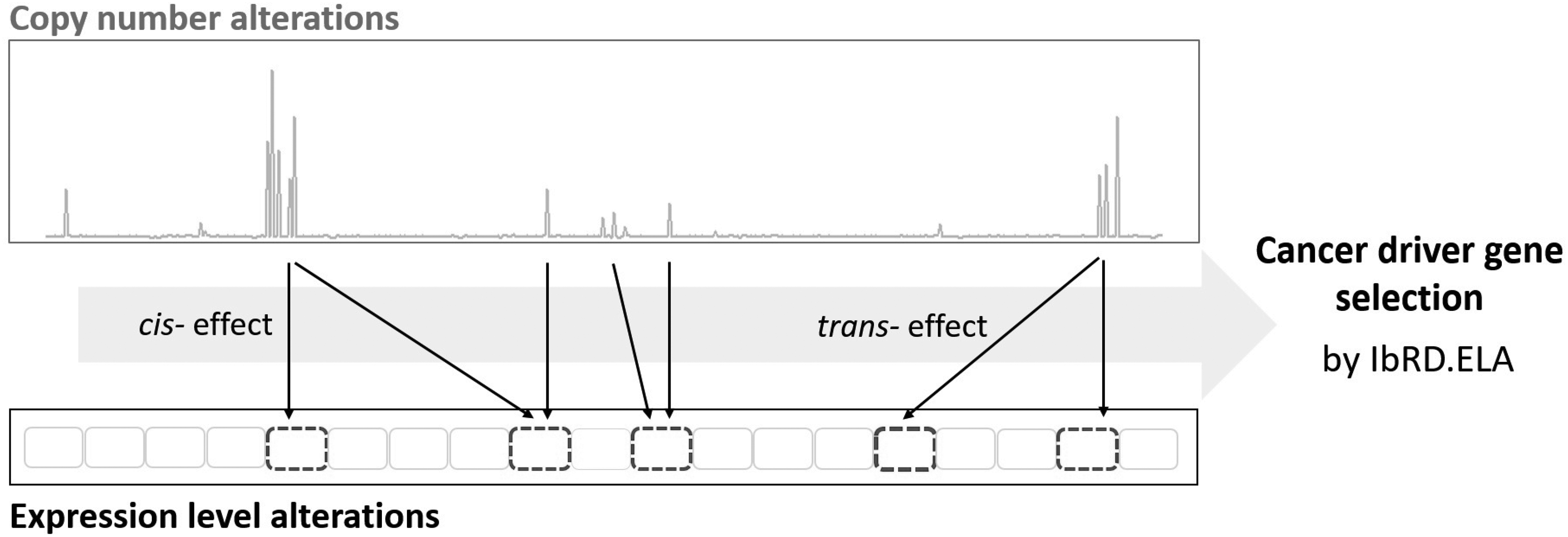
Driver gene selection is crucial to understand the heterogeneous system of cancer. To identity cancer driver genes, various statistical strategies have been proposed, especially the L1-type regularization methods have drawn a large amount of attention. However, the statistical approaches have been developed purely from algorithmic and statistical point, and the existing studies have applied the statistical approaches to genomic data analysis without consideration of biological knowledge. We consider a statistical strategy incorporating biological knowledge to identify cancer driver gene. The alterations of copy number have been considered to driver cancer pathogenesis processes, and the region of strong interaction of copy number alterations and expression levels was known as a tumor-related symptom. We incorporate the influence of copy number alterations on expression levels to cancer driver gene-selection processes. To quantify the dependence of copy number alterations on expression levels, we consider \documentclass{aastex}\usepackage{amsbsy}\usepackage{amsfonts}\usepackage{amssymb}\usepackage{bm}\usepackage{mathrsfs}\usepackage{pifont}\usepackage{stmaryrd}\usepackage{textcomp}\usepackage{portland, xspace}\usepackage{amsmath, amsxtra}\pagestyle{empty}\DeclareMathSizes{10}{9}{7}{6}\begin{document}
${\textbf{\textit{cis}}} -$
\end{document} and \documentclass{aastex}\usepackage{amsbsy}\usepackage{amsfonts}\usepackage{amssymb}\usepackage{bm}\usepackage{mathrsfs}\usepackage{pifont}\usepackage{stmaryrd}\usepackage{textcomp}\usepackage{portland, xspace}\usepackage{amsmath, amsxtra}\pagestyle{empty}\DeclareMathSizes{10}{9}{7}{6}\begin{document}
${\textbf{\textit{trans}}} -$
\end{document} effects of copy number alterations on expression levels of genes, and incorporate the symptom of tumor pathogenesis to gene-selection procedures. We then proposed an interaction-based feature-selection strategy based on the adaptiveL1-type regularization and random lasso procedures. The proposed method imposes a large amount of penalty on genes corresponding to a low dependency of the two features, thus the coefficients of the genes are estimated to be small or exactly 0. It implies that the proposed method can provide biologically relevant results in cancer driver gene selection. Monte Carlo simulations and analysis of the Cancer Genome Atlas (TCGA) data show that the proposed strategy is effective for high-dimensional genomic data analysis. Furthermore, the proposed method provides reliable and biologically relevant results for cancer driver gene selection in TCGA data analysis.
1. Introduction
The crucial issue in genomic research is to identify driver genes involved in diseases (e.g., cancer). To identify the cancer driver genes, various statistical methods have been proposed and widely used in the fields of bioinformatics. The L1-type regularization methods, for example, lasso (Tibshirani, 1996), adaptive lasso (Zou, 2006), elastic net (Zou and Hastie, 2008), and random lasso (Wang et al., 2011), have drawn considerable attention for genomic data analysis (e.g., driver gene identification). By imposing the L1-type penalty to the least squares loss function and likelihood function, the lasso-type approaches can perform variable selection and model estimation simultaneously. The elastic net especially has been often used to gene selection, because the method can select variables more than sample size n. In other words, the elastic net effectively performs feature selection in high-dimensional data situation. Ghosh and Chinnaiyan (2005) applied the lasso to identify biomarkers in prostate cancer tissue classification. Algamal and Lee (2015) performed gene selection and cancer classification by using the adaptive lasso in line with the penalized logistic regression. Waldmann et al. (2013) applied the lasso and elastic net to genome-wide association studies. In addition to these, various L1-type approaches have been applied to genomic data analysis (Lin et al., 2013; Das et al., 2015). Although the lasso-type approaches have provided effective results in regression modeling, the methods suffer from a few demerits: erroneous estimation results, limitations of subset size, and so on, especially in the presence of multicollinearity (Wang et al., 2011).
To resolve these issues, Wang et al. (2011) proposed the random lasso based on the random forest method in bootstrap regression modeling. By using the random forest procedure in each bootstrap regression modeling, the random lasso performs regression modeling based only on a small set of highly correlated predictor variables, and thus we can resolve the demerits caused by multicollinearity. Furthermore, the random lasso can select features more than sample size n, since the feature-selection result is an aggregation of the B results of the bootstrap regression modeling. The existing L1-type regularization methods (e.g., lasso, elastic net, and random lasso), however, were developed purely from algorithmic and statistical point. In other words, we cannot incorporate a biological information into genomic data analysis, even though much biological knowledge is available. However, incorporation of the knowledge about a data set is crucial and leads to interpretable modeling results.
We consider a driver gene selection incorporating biological knowledge. The alterations of copy number are characteristic of cancers, and have been considered to driver cancer pathogenesis processes (Lipson et al., 2004). Although it was well known that the copy number alterations localize to regions harboring oncogenes or tumor suppressors and expression levels of driver genes are influenced by the copy number alterations (Yuan et al., 2012), relatively little attention was paid to the incorporation of the symptom into cancer driver gene-selection procedures. Furthermore, the driver gene selection in the existing studies has been performed based only on expression levels of genes, even though various large-scale omics projects (e.g., The Cancer Genome Project and The Cancer Genome Atlas [TCGA]) have provided not only expression levels but also various genome scale information (e.g., mRNA and microRNA expression, DNA copy number and methylation, and DNA sequence).
We develop an interaction-based variable selection strategy for uncovering cancer driver genes. We consider the influence of copy number alterations on expression levels as a symptom of a cancer pathogenesis, and incorporate the symptom into cancer driver gene selection. To quantity the association of the two factors (i.e., expression levels and copy number alterations), we measure both \documentclass{aastex}\usepackage{amsbsy}\usepackage{amsfonts}\usepackage{amssymb}\usepackage{bm}\usepackage{mathrsfs}\usepackage{pifont}\usepackage{stmaryrd}\usepackage{textcomp}\usepackage{portland, xspace}\usepackage{amsmath, amsxtra}\pagestyle{empty}\DeclareMathSizes{10}{9}{7}{6}\begin{document}
$$cis -$$
\end{document} and \documentclass{aastex}\usepackage{amsbsy}\usepackage{amsfonts}\usepackage{amssymb}\usepackage{bm}\usepackage{mathrsfs}\usepackage{pifont}\usepackage{stmaryrd}\usepackage{textcomp}\usepackage{portland, xspace}\usepackage{amsmath, amsxtra}\pagestyle{empty}\DeclareMathSizes{10}{9}{7}{6}\begin{document}
$$trans -$$
\end{document} effects of copy number alteration on expression levels as shown in Figure 1, and consider a score taking an amount of the association in line with Yuan et al. (2012). We then propose an interaction-based random elastic net (IbRD.ELA) in line with the random lasso procedures. The proposed method discriminately imposes the L1-type penalty on each gene depending on an amount of dependency of the copy number alterations on expression levels of a gene. The incorporation of the dependency into gene-selection procedures enables us to impose a large amount of penalty on the genes corresponding to the low dependency between the two genome scale information, and thus the genes are easily deleted from the model. It implies that the proposed method can provide interpretable gene-selection results in cancer research, and thus we can effectively uncover cancer driver genes. Furthermore, the proposed IbRD.ELA can efficiently perform high-dimensional regression modeling even in the presence of multicollinearity between the predictor variables, since the IbRD.ELA is based on random forest method and bootstrap regression modeling.
The expression levels of genes are affected by changes of copy number alterations in line with \documentclass{aastex}\usepackage{amsbsy}\usepackage{amsfonts}\usepackage{amssymb}\usepackage{bm}\usepackage{mathrsfs}\usepackage{pifont}\usepackage{stmaryrd}\usepackage{textcomp}\usepackage{portland, xspace}\usepackage{amsmath, amsxtra}\pagestyle{empty}\DeclareMathSizes{10}{9}{7}{6}\begin{document}
$$cis -$$
\end{document} and \documentclass{aastex}\usepackage{amsbsy}\usepackage{amsfonts}\usepackage{amssymb}\usepackage{bm}\usepackage{mathrsfs}\usepackage{pifont}\usepackage{stmaryrd}\usepackage{textcomp}\usepackage{portland, xspace}\usepackage{amsmath, amsxtra}\pagestyle{empty}\DeclareMathSizes{10}{9}{7}{6}\begin{document}
$$trans -$$
\end{document} effects (Yuan et al., 2012). The genes corresponding to a strong dependency of copy number alterations on expression levels play a key role in driving tumor pathogenesis. IbRD.ELA, interaction-based random elastic net.
We demonstrate through Monte Carlo simulations the effectiveness of the proposed IbRD.ELA for high-dimensional regression modeling. We also apply the IbRD.ELA to TCGA data analysis to show the biological reliability of the proposed strategy. Numerical studies show that the proposed IbRD.ELA outperforms high-dimensional genomic data analysis in the viewpoint of feature selection and predictive accuracy.
The rest of this article is organized as follows. In Section 2, we introduce the existing L1-type regularization methods and propose the interaction-based feature-selection method (i.e., IbRD.ELA). Section 3 demonstrates through Monte Carlo experiments the effectiveness of the proposed method. The real-world example based on TCGA data analysis is shown in Section 4. We state our conclusions in Section 5.
2. Method
Suppose we have n independent observations \documentclass{aastex}\usepackage{amsbsy}\usepackage{amsfonts}\usepackage{amssymb}\usepackage{bm}\usepackage{mathrsfs}\usepackage{pifont}\usepackage{stmaryrd}\usepackage{textcomp}\usepackage{portland, xspace}\usepackage{amsmath, amsxtra}\pagestyle{empty}\DeclareMathSizes{10}{9}{7}{6}\begin{document}
$$\{ ( {y_i},{\textbf{\textit{x}}_i} ); i = 1 , \ldots , n \} $$
\end{document}, where yi are random response variables and \documentclass{aastex}\usepackage{amsbsy}\usepackage{amsfonts}\usepackage{amssymb}\usepackage{bm}\usepackage{mathrsfs}\usepackage{pifont}\usepackage{stmaryrd}\usepackage{textcomp}\usepackage{portland, xspace}\usepackage{amsmath, amsxtra}\pagestyle{empty}\DeclareMathSizes{10}{9}{7}{6}\begin{document}
$\textbf{\textit{x}}_{\textbf{\textit{i}}}$
\end{document} are p-dimensional vectors of the predictor variables. Consider the linear regression model,
\documentclass{aastex}\usepackage{amsbsy}\usepackage{amsfonts}\usepackage{amssymb}\usepackage{bm}\usepackage{mathrsfs}\usepackage{pifont}\usepackage{stmaryrd}\usepackage{textcomp}\usepackage{portland, xspace}\usepackage{amsmath, amsxtra}\pagestyle{empty}\DeclareMathSizes{10}{9}{7}{6}\begin{document}
\begin{align*}
{y_i} = \textbf{\textit{x}}_i^T{ \beta} + { \varepsilon _i}, \quad i = 1 , \ldots , n , \tag{1}
\end{align*}
\end{document}
where \documentclass{aastex}\usepackage{amsbsy}\usepackage{amsfonts}\usepackage{amssymb}\usepackage{bm}\usepackage{mathrsfs}\usepackage{pifont}\usepackage{stmaryrd}\usepackage{textcomp}\usepackage{portland, xspace}\usepackage{amsmath, amsxtra}\pagestyle{empty}\DeclareMathSizes{10}{9}{7}{6}\begin{document}
$$\beta$$
\end{document} is an unknown p-dimensional vector of regression coefficients and \documentclass{aastex}\usepackage{amsbsy}\usepackage{amsfonts}\usepackage{amssymb}\usepackage{bm}\usepackage{mathrsfs}\usepackage{pifont}\usepackage{stmaryrd}\usepackage{textcomp}\usepackage{portland, xspace}\usepackage{amsmath, amsxtra}\pagestyle{empty}\DeclareMathSizes{10}{9}{7}{6}\begin{document}
$${ \varepsilon _i}$$
\end{document} are the random errors that are assumed to be independently and identically distributed with mean 0 and variance \documentclass{aastex}\usepackage{amsbsy}\usepackage{amsfonts}\usepackage{amssymb}\usepackage{bm}\usepackage{mathrsfs}\usepackage{pifont}\usepackage{stmaryrd}\usepackage{textcomp}\usepackage{portland, xspace}\usepackage{amsmath, amsxtra}\pagestyle{empty}\DeclareMathSizes{10}{9}{7}{6}\begin{document}
$${ \sigma ^2}$$
\end{document}.
For the linear regression modeling, the L1-type regularization methods (e.g., lasso and elastic net) have drawn a large amount of attention,
\documentclass{aastex}\usepackage{amsbsy}\usepackage{amsfonts}\usepackage{amssymb}\usepackage{bm}\usepackage{mathrsfs}\usepackage{pifont}\usepackage{stmaryrd}\usepackage{textcomp}\usepackage{portland, xspace}\usepackage{amsmath, amsxtra}\pagestyle{empty}\DeclareMathSizes{10}{9}{7}{6}\begin{document}
\begin{align*}
{ \hat { \beta} ^{L1}} = \mathop {{ \rm{arg \ min}}} \limits_ \beta \left\{ \sum \limits_{i = 1}^n { ( {y_i} - \textbf{\textit{x}}_i^T{ \beta} ) ^2} + {P_ \lambda } ( {\beta} ) \right\} , \tag{2}
\end{align*}
\end{document}
where \documentclass{aastex}\usepackage{amsbsy}\usepackage{amsfonts}\usepackage{amssymb}\usepackage{bm}\usepackage{mathrsfs}\usepackage{pifont}\usepackage{stmaryrd}\usepackage{textcomp}\usepackage{portland, xspace}\usepackage{amsmath, amsxtra}\pagestyle{empty}\DeclareMathSizes{10}{9}{7}{6}\begin{document}
$${{\bold P}_ \lambda } ( {\beta} )$$
\end{document} is an L1-type penalty, such as
where \documentclass{aastex}\usepackage{amsbsy}\usepackage{amsfonts}\usepackage{amssymb}\usepackage{bm}\usepackage{mathrsfs}\usepackage{pifont}\usepackage{stmaryrd}\usepackage{textcomp}\usepackage{portland, xspace}\usepackage{amsmath, amsxtra}\pagestyle{empty}\DeclareMathSizes{10}{9}{7}{6}\begin{document}
$$\lambda$$
\end{document} is a tuning parameter controlling model complexity and \documentclass{aastex}\usepackage{amsbsy}\usepackage{amsfonts}\usepackage{amssymb}\usepackage{bm}\usepackage{mathrsfs}\usepackage{pifont}\usepackage{stmaryrd}\usepackage{textcomp}\usepackage{portland, xspace}\usepackage{amsmath, amsxtra}\pagestyle{empty}\DeclareMathSizes{10}{9}{7}{6}\begin{document}
$$\alpha > 0$$
\end{document}. By imposing the L1-type penalties to the least squares loss function, the lasso-type methods can perform simultaneous variable selection and model estimation. Furthermore, the methods provide stable estimation results even in the presence of multicollinearity between predictor variables.
Although the L1-type regularization approaches provide effective regression modeling results, the methods suffer from the following demerits (Wang et al., 2011; Park et al., 2015).
• When \documentclass{aastex}\usepackage{amsbsy}\usepackage{amsfonts}\usepackage{amssymb}\usepackage{bm}\usepackage{mathrsfs}\usepackage{pifont}\usepackage{stmaryrd}\usepackage{textcomp}\usepackage{portland, xspace}\usepackage{amsmath, amsxtra}\pagestyle{empty}\DeclareMathSizes{10}{9}{7}{6}\begin{document}
$$p > n$$
\end{document}, the lasso and adaptive lasso can select at most n variables because of the convex optimization problem. This implies that the lasso and adaptive lasso are not suitable tools for high-dimensional data (i.e., p≫n) analysis.
• The lasso tends to pick only one variable from among several highly correlated variables, even if all are related to a response variable, because the method cannot account for grouping effect of predictor variables. This implies that the lasso is not suitable for genomic data analysis, since the genomic alterations of genes (e.g., expression levels, copy number alterations, and methylation) that share a common biological pathway are usually highly correlated. However, the lasso selects only one gene, even though several genes are associated with a complex cancer mechanism considered to be the response variable.
• The elastic net may lead to erroneous estimation results for coefficients of highly correlated predictor variables with different magnitudes, especially those with different signs, because of its “grouping effect”. However, coefficients of highly correlated variables with different magnitudes are frequently observed in bioinformatics research, since genes in the common biological pathway are usually highly correlated, and their regression coefficients can have different magnitudes or a different sign. It implies that the elastic net may lead to erroneous estimation results in genomic data analysis.
To resolve the problems, Wang et al. (2011) proposed the random lasso, which is constructed by two steps of bootstrap regression modeling as follows:
• Step 1: Computing importance measures of predictor variables.
1. Draw B bootstrap samples with size n by sampling with replacement from the original data set.
2. For the \documentclass{aastex}\usepackage{amsbsy}\usepackage{amsfonts}\usepackage{amssymb}\usepackage{bm}\usepackage{mathrsfs}\usepackage{pifont}\usepackage{stmaryrd}\usepackage{textcomp}\usepackage{portland, xspace}\usepackage{amsmath, amsxtra}\pagestyle{empty}\DeclareMathSizes{10}{9}{7}{6}\begin{document}
$$b_1^{th}$$
\end{document} bootstrap sample, \documentclass{aastex}\usepackage{amsbsy}\usepackage{amsfonts}\usepackage{amssymb}\usepackage{bm}\usepackage{mathrsfs}\usepackage{pifont}\usepackage{stmaryrd}\usepackage{textcomp}\usepackage{portland, xspace}\usepackage{amsmath, amsxtra}\pagestyle{empty}\DeclareMathSizes{10}{9}{7}{6}\begin{document}
$${b_1} \in \{ 1 , 2 , \ldots , B \} $$
\end{document}, randomly select q1 candidate variables, and the lasso is applied to estimate coefficients \documentclass{aastex}\usepackage{amsbsy}\usepackage{amsfonts}\usepackage{amssymb}\usepackage{bm}\usepackage{mathrsfs}\usepackage{pifont}\usepackage{stmaryrd}\usepackage{textcomp}\usepackage{portland, xspace}\usepackage{amsmath, amsxtra}\pagestyle{empty}\DeclareMathSizes{10}{9}{7}{6}\begin{document}
$$\hat \beta _j^{ ( {b_1} ) }$$
\end{document} for \documentclass{aastex}\usepackage{amsbsy}\usepackage{amsfonts}\usepackage{amssymb}\usepackage{bm}\usepackage{mathrsfs}\usepackage{pifont}\usepackage{stmaryrd}\usepackage{textcomp}\usepackage{portland, xspace}\usepackage{amsmath, amsxtra}\pagestyle{empty}\DeclareMathSizes{10}{9}{7}{6}\begin{document}
$$j = 1 , \ldots , p$$
\end{document}.
Wang et al. (2011) also considered a threshold \documentclass{aastex}\usepackage{amsbsy}\usepackage{amsfonts}\usepackage{amssymb}\usepackage{bm}\usepackage{mathrsfs}\usepackage{pifont}\usepackage{stmaryrd}\usepackage{textcomp}\usepackage{portland, xspace}\usepackage{amsmath, amsxtra}\pagestyle{empty}\DeclareMathSizes{10}{9}{7}{6}\begin{document}
$${t_n} = 1 / n$$
\end{document} for final feature selection, because the mentioned procedures of the random lasso may suffer from false positive in feature selection (i.e., some of the estimated nonzero coefficients may result from a particular bootstrap sample). In other words, Wang et al. (2011) considered an additional feature selection based on the threshold, that is, the predictor variables with |βj| ⩽ tn are deleted from the model. The random lasso based on the random forest approach can overcome the drawback caused by multicollinearity between predictor variables, since only a small set of highly correlated variables may be considered as predictor variables in each bootstrap regression modeling. Furthermore, the method can select many predictor variables more than sample size n (i.e., the random lasso can overcome the limitation of subset size of the lasso and adaptive lasso), because the feature-selection result is an aggregation of bootstrap regression modeling results for B bootstrap samples.
The random lasso, however, was developed purely from algorithmic point without consideration of any biological knowledge. In a variable selection procedure, considering knowledge of the data set is a crucial issue, and incorporating the knowledge leads to effective and interpretable analysis results.
2.1. Interaction-based random elastic net
For interpretable and effective driver gene selection, we incorporate a biological knowledge into feature-selection procedures. The copy number alterations have been considered to a typical characteristic of cancer, and it was well known that the influence of copy number alterations on expression levels is a crucial symptom of tumor pathogenesis. Thus, we incorporate the influence of copy number alterations on expression levels into cancer driver gene-selection procedures.
We consider \documentclass{aastex}\usepackage{amsbsy}\usepackage{amsfonts}\usepackage{amssymb}\usepackage{bm}\usepackage{mathrsfs}\usepackage{pifont}\usepackage{stmaryrd}\usepackage{textcomp}\usepackage{portland, xspace}\usepackage{amsmath, amsxtra}\pagestyle{empty}\DeclareMathSizes{10}{9}{7}{6}\begin{document}
$$cis -$$
\end{document} and \documentclass{aastex}\usepackage{amsbsy}\usepackage{amsfonts}\usepackage{amssymb}\usepackage{bm}\usepackage{mathrsfs}\usepackage{pifont}\usepackage{stmaryrd}\usepackage{textcomp}\usepackage{portland, xspace}\usepackage{amsmath, amsxtra}\pagestyle{empty}\DeclareMathSizes{10}{9}{7}{6}\begin{document}
$$trans -$$
\end{document} effects of the copy number alterations on expression levels as an association of the two genome scale information (Yuan et al., 2012),
• \documentclass{aastex}\usepackage{amsbsy}\usepackage{amsfonts}\usepackage{amssymb}\usepackage{bm}\usepackage{mathrsfs}\usepackage{pifont}\usepackage{stmaryrd}\usepackage{textcomp}\usepackage{portland, xspace}\usepackage{amsmath, amsxtra}\pagestyle{empty}\DeclareMathSizes{10}{9}{7}{6}\begin{document}
$$cis -$$
\end{document} effect: copy number alteration in proximal genes within a several Mb window has an influence on gene expression.
• \documentclass{aastex}\usepackage{amsbsy}\usepackage{amsfonts}\usepackage{amssymb}\usepackage{bm}\usepackage{mathrsfs}\usepackage{pifont}\usepackage{stmaryrd}\usepackage{textcomp}\usepackage{portland, xspace}\usepackage{amsmath, amsxtra}\pagestyle{empty}\DeclareMathSizes{10}{9}{7}{6}\begin{document}
$$trans -$$
\end{document} effect: remote alteration of copy number influence on gene expression.
To quantify the association, we refer to the method proposed by Yuan et al. (2012), and consider a score taking an amount of the association between expression levels and copy number alterations.
The linear regression model for a gene k is give as
\documentclass{aastex}\usepackage{amsbsy}\usepackage{amsfonts}\usepackage{amssymb}\usepackage{bm}\usepackage{mathrsfs}\usepackage{pifont}\usepackage{stmaryrd}\usepackage{textcomp}\usepackage{portland, xspace}\usepackage{amsmath, amsxtra}\pagestyle{empty}\DeclareMathSizes{10}{9}{7}{6}\begin{document}
\begin{align*}
{\textbf{\textit{x}}_k} = \textbf{\textit{ Z}}{ \gamma _k} + { {\bm{\varepsilon}} _k}, \quad k = 1 , \ldots , p , \tag{3}
\end{align*}
\end{document}
where \documentclass{aastex}\usepackage{amsbsy}\usepackage{amsfonts}\usepackage{amssymb}\usepackage{bm}\usepackage{mathrsfs}\usepackage{pifont}\usepackage{stmaryrd}\usepackage{textcomp}\usepackage{portland, xspace}\usepackage{amsmath, amsxtra}\pagestyle{empty}\DeclareMathSizes{10}{9}{7}{6}\begin{document}
$${ \bm{\varepsilon} _k} = ( { \bm{\varepsilon} _{1k}},{ \bm{\varepsilon} _{2k}}, \ldots , { \bm{\varepsilon} _{nk}} )$$
\end{document} are the random errors, \documentclass{aastex}\usepackage{amsbsy}\usepackage{amsfonts}\usepackage{amssymb}\usepackage{bm}\usepackage{mathrsfs}\usepackage{pifont}\usepackage{stmaryrd}\usepackage{textcomp}\usepackage{portland, xspace}\usepackage{amsmath, amsxtra}\pagestyle{empty}\DeclareMathSizes{10}{9}{7}{6}\begin{document}
$$\textbf{\textit{ Z}} = ( {\textbf{\textit{ z}}_1},{\textbf{\textit{ z}}_2}, \ldots , {\textbf{\textit{ z}}_p} )$$
\end{document} are copy number alterations of p DNA regions, and \documentclass{aastex}\usepackage{amsbsy}\usepackage{amsfonts}\usepackage{amssymb}\usepackage{bm}\usepackage{mathrsfs}\usepackage{pifont}\usepackage{stmaryrd}\usepackage{textcomp}\usepackage{portland, xspace}\usepackage{amsmath, amsxtra}\pagestyle{empty}\DeclareMathSizes{10}{9}{7}{6}\begin{document}
$${\textbf{\textit{ x}}_k} = ( {x_{1k}},{x_{2k}}, \ldots , {x_{nk}}{ ) ^T}$$
\end{document} are expression levels of a gene k for n samples. In the linear regression model, the expression levels and copy number alterations are considered as response and predictor variables, respectively. For gene k, the elastic net is applied to estimate the regression coefficient \documentclass{aastex}\usepackage{amsbsy}\usepackage{amsfonts}\usepackage{amssymb}\usepackage{bm}\usepackage{mathrsfs}\usepackage{pifont}\usepackage{stmaryrd}\usepackage{textcomp}\usepackage{portland, xspace}\usepackage{amsmath, amsxtra}\pagestyle{empty}\DeclareMathSizes{10}{9}{7}{6}\begin{document}
$${{ \gamma }_k}$$
\end{document},
\documentclass{aastex}\usepackage{amsbsy}\usepackage{amsfonts}\usepackage{amssymb}\usepackage{bm}\usepackage{mathrsfs}\usepackage{pifont}\usepackage{stmaryrd}\usepackage{textcomp}\usepackage{portland, xspace}\usepackage{amsmath, amsxtra}\pagestyle{empty}\DeclareMathSizes{10}{9}{7}{6}\begin{document}
\begin{align*}
{\hat {\gamma}_k} = \mathop {{ \rm{arg \ min}}} \limits_{{ \gamma
_k}} \left\{ \sum \limits_{i = 1}^n { (
\textbf{\textit{x}}_\textbf{\textit{ik}} -
\textbf{\textit{z}}_i^T{ \gamma _k} ) ^2} + \lambda \{ ( 1 -
\alpha ) \sum \limits_{j = 1}^p \vert { \gamma _{kj}} \vert +
\alpha \sum \limits_{j = 1}^p \, \gamma _{kj}^2 \right\} , \tag{4}
\end{align*}
\end{document}
where \documentclass{aastex}\usepackage{amsbsy}\usepackage{amsfonts}\usepackage{amssymb}\usepackage{bm}\usepackage{mathrsfs}\usepackage{pifont}\usepackage{stmaryrd}\usepackage{textcomp}\usepackage{portland, xspace}\usepackage{amsmath, amsxtra}\pagestyle{empty}\DeclareMathSizes{10}{9}{7}{6}\begin{document}
$${{ z}_i}$$
\end{document} are p-dimensional vectors. We then compute the following residuals:
\documentclass{aastex}\usepackage{amsbsy}\usepackage{amsfonts}\usepackage{amssymb}\usepackage{bm}\usepackage{mathrsfs}\usepackage{pifont}\usepackage{stmaryrd}\usepackage{textcomp}\usepackage{portland, xspace}\usepackage{amsmath, amsxtra}\pagestyle{empty}\DeclareMathSizes{10}{9}{7}{6}\begin{document}
\begin{align*}
{\textbf{\textit{x}}_k} = {{ \bm{\varepsilon}}_k}, \tag{5}
\end{align*}
\end{document}\documentclass{aastex}\usepackage{amsbsy}\usepackage{amsfonts}\usepackage{amssymb}\usepackage{bm}\usepackage{mathrsfs}\usepackage{pifont}\usepackage{stmaryrd}\usepackage{textcomp}\usepackage{portland, xspace}\usepackage{amsmath, amsxtra}\pagestyle{empty}\DeclareMathSizes{10}{9}{7}{6}\begin{document}
\begin{align*}
{\textbf{\textit{ x}}_k} = \sum \limits_{j = 1}^p \,{\textbf{\textit{z}}_j}{ \hat { \gamma} _j} + {{ \bm{\varepsilon}}^{\prime}_k}. \tag{6}
\end{align*}
\end{document}
The amount of dependency of copy number alterations on expression levels in both \documentclass{aastex}\usepackage{amsbsy}\usepackage{amsfonts}\usepackage{amssymb}\usepackage{bm}\usepackage{mathrsfs}\usepackage{pifont}\usepackage{stmaryrd}\usepackage{textcomp}\usepackage{portland, xspace}\usepackage{amsmath, amsxtra}\pagestyle{empty}\DeclareMathSizes{10}{9}{7}{6}\begin{document}
$$cis -$$
\end{document} and \documentclass{aastex}\usepackage{amsbsy}\usepackage{amsfonts}\usepackage{amssymb}\usepackage{bm}\usepackage{mathrsfs}\usepackage{pifont}\usepackage{stmaryrd}\usepackage{textcomp}\usepackage{portland, xspace}\usepackage{amsmath, amsxtra}\pagestyle{empty}\DeclareMathSizes{10}{9}{7}{6}\begin{document}
$$trans - $$
\end{document} effects (i.e., copy number dependency score) is measured as follows:
\documentclass{aastex}\usepackage{amsbsy}\usepackage{amsfonts}\usepackage{amssymb}\usepackage{bm}\usepackage{mathrsfs}\usepackage{pifont}\usepackage{stmaryrd}\usepackage{textcomp}\usepackage{portland, xspace}\usepackage{amsmath, amsxtra}\pagestyle{empty}\DeclareMathSizes{10}{9}{7}{6}\begin{document}
\begin{align*}
Score_k^ { both } = 1 - { \frac { \bm { \sigma } _ { { { \ \bm {
\varepsilon } ^ { \prime } } _k } } ^2 } { \ \bm { \sigma } _ { {
\ \bm { \varepsilon } _k } } ^2 } } . \tag { 7 }
\end{align*}
\end{document}
A large value of the \documentclass{aastex}\usepackage{amsbsy}\usepackage{amsfonts}\usepackage{amssymb}\usepackage{bm}\usepackage{mathrsfs}\usepackage{pifont}\usepackage{stmaryrd}\usepackage{textcomp}\usepackage{portland, xspace}\usepackage{amsmath, amsxtra}\pagestyle{empty}\DeclareMathSizes{10}{9}{7}{6}\begin{document}
$$Score_k^{both}$$
\end{document} indicates that a large proportion of variations of expression levels for gene k is explained by copy number alterations. Thus, the gene corresponding to a larger value of the score can be considered as a cancer driver gene.
We then consider a weight for the adaptive L1-type penalty. To prevent that a weight excessively dominates feature-selection procedures, we consider a weight wk with range between L and U as follows:
\documentclass{aastex}\usepackage{amsbsy}\usepackage{amsfonts}\usepackage{amssymb}\usepackage{bm}\usepackage{mathrsfs}\usepackage{pifont}\usepackage{stmaryrd}\usepackage{textcomp}\usepackage{portland, xspace}\usepackage{amsmath, amsxtra}\pagestyle{empty}\DeclareMathSizes{10}{9}{7}{6}\begin{document}
\begin{align*}
w_k^b = 1 \bigg/ \left( \frac { 1 } { U } + { \frac { \big[ \{
Score_k^ { both } - { \rm { min } } ( Score_k^ { both } ) \} (
\frac { 1 } { L } - \frac { 1 } { U } ) \big] } { { \rm { max }
} ( Score_k^ { both } ) - { \rm { min } } ( Score_k^ { both } ) }
} \right), \quad \, \,j = 1 , \ldots , p. \tag { 8 }
\end{align*}
\end{document}
We then proposed an interaction-based L1-type regularization method based on the weight, which adjusts an amount of the L1-type penalty imposed to each gene, as follows.
Ib.ELA imposes a large amount of penalty to a gene corresponding to a small value of the score. In other words, the genes having relatively low dependency of copy number alterations on expression levels receive a large amount of penalty, and thus the coefficients of the genes may be estimated to be small or exactly 0. In contrast, the genes corresponding to high dependency of the two factors (i.e., the large value of the score) receive a small amount of the penalty, and thus the coefficients of the genes are estimated to be large.
We then propose an interaction-based random elastic net (IbRD.ELA(B)) based on Ib.ELA(B) in line with the random lasso. The IbRD.ELA(B) is implemented by the following Algorithm 1:
Algorithm 1Interaction-based random elastic net (IbRD.ELA(B))
• Step 1: Measuring the copy number dependency score (\documentclass{aastex}\usepackage{amsbsy}\usepackage{amsfonts}\usepackage{amssymb}\usepackage{bm}\usepackage{mathrsfs}\usepackage{pifont}\usepackage{stmaryrd}\usepackage{textcomp}\usepackage{portland, xspace}\usepackage{amsmath, amsxtra}\pagestyle{empty}\DeclareMathSizes{10}{9}{7}{6}\begin{document}
$$Score_k^{both}$$
\end{document}) of genes.
1. Draw B bootstrap samples with size n by sampling with replacement from the original data set.
2. For the \documentclass{aastex}\usepackage{amsbsy}\usepackage{amsfonts}\usepackage{amssymb}\usepackage{bm}\usepackage{mathrsfs}\usepackage{pifont}\usepackage{stmaryrd}\usepackage{textcomp}\usepackage{portland, xspace}\usepackage{amsmath, amsxtra}\pagestyle{empty}\DeclareMathSizes{10}{9}{7}{6}\begin{document}
$$b_1^{th}$$
\end{document} bootstrap sample, \documentclass{aastex}\usepackage{amsbsy}\usepackage{amsfonts}\usepackage{amssymb}\usepackage{bm}\usepackage{mathrsfs}\usepackage{pifont}\usepackage{stmaryrd}\usepackage{textcomp}\usepackage{portland, xspace}\usepackage{amsmath, amsxtra}\pagestyle{empty}\DeclareMathSizes{10}{9}{7}{6}\begin{document}
$${b_1} \in \{ 1 , 2 , \ldots , B \} $$
\end{document}, q1 candidate variables are randomly selected, and Ib.ELA(B) is applied to the regression modeling, and we obtain estimators \documentclass{aastex}\usepackage{amsbsy}\usepackage{amsfonts}\usepackage{amssymb}\usepackage{bm}\usepackage{mathrsfs}\usepackage{pifont}\usepackage{stmaryrd}\usepackage{textcomp}\usepackage{portland, xspace}\usepackage{amsmath, amsxtra}\pagestyle{empty}\DeclareMathSizes{10}{9}{7}{6}\begin{document}
$$\hat \beta _j^{ ( {b_1} ) }$$
\end{document} for \documentclass{aastex}\usepackage{amsbsy}\usepackage{amsfonts}\usepackage{amssymb}\usepackage{bm}\usepackage{mathrsfs}\usepackage{pifont}\usepackage{stmaryrd}\usepackage{textcomp}\usepackage{portland, xspace}\usepackage{amsmath, amsxtra}\pagestyle{empty}\DeclareMathSizes{10}{9}{7}{6}\begin{document}
$$j = 1 , \ldots , p$$
\end{document}, respectively.
3. The importance measures of xj are calculated as \documentclass{aastex}\usepackage{amsbsy}\usepackage{amsfonts}\usepackage{amssymb}\usepackage{bm}\usepackage{mathrsfs}\usepackage{pifont}\usepackage{stmaryrd}\usepackage{textcomp}\usepackage{portland, xspace}\usepackage{amsmath, amsxtra}\pagestyle{empty}\DeclareMathSizes{10}{9}{7}{6}\begin{document}
$${I_j} = \, \, \vert {B^{ - 1}} \sum \nolimits_{{b_1} = 1}^B \, \, \hat \beta _j^{ ( {b_1} ) } \vert$$
\end{document}.
• Step 3: Estimation and variable selection
1. Draw B bootstrap samples with size n by sampling with replacement from the original data set.
2. For each \documentclass{aastex}\usepackage{amsbsy}\usepackage{amsfonts}\usepackage{amssymb}\usepackage{bm}\usepackage{mathrsfs}\usepackage{pifont}\usepackage{stmaryrd}\usepackage{textcomp}\usepackage{portland, xspace}\usepackage{amsmath, amsxtra}\pagestyle{empty}\DeclareMathSizes{10}{9}{7}{6}\begin{document}
$$b_2^{th}$$
\end{document} bootstrap sample for IbRD.ELA(B), \documentclass{aastex}\usepackage{amsbsy}\usepackage{amsfonts}\usepackage{amssymb}\usepackage{bm}\usepackage{mathrsfs}\usepackage{pifont}\usepackage{stmaryrd}\usepackage{textcomp}\usepackage{portland, xspace}\usepackage{amsmath, amsxtra}\pagestyle{empty}\DeclareMathSizes{10}{9}{7}{6}\begin{document}
$${b_2} \in \{ 1 , 2 , \ldots , B \} $$
\end{document}, q2 candidate variables are randomly selected with a selection probability of xj proportional to Ij. And, Ib.ELA is applied for regression modeling, and we obtain the estimator \documentclass{aastex}\usepackage{amsbsy}\usepackage{amsfonts}\usepackage{amssymb}\usepackage{bm}\usepackage{mathrsfs}\usepackage{pifont}\usepackage{stmaryrd}\usepackage{textcomp}\usepackage{portland, xspace}\usepackage{amsmath, amsxtra}\pagestyle{empty}\DeclareMathSizes{10}{9}{7}{6}\begin{document}
$$\hat \beta _j^{ ( {b_2} ) }$$
\end{document}.
To overcome the false positive results of the random lasso procedures, Wang et al. (2011) considered the threshold \documentclass{aastex}\usepackage{amsbsy}\usepackage{amsfonts}\usepackage{amssymb}\usepackage{bm}\usepackage{mathrsfs}\usepackage{pifont}\usepackage{stmaryrd}\usepackage{textcomp}\usepackage{portland, xspace}\usepackage{amsmath, amsxtra}\pagestyle{empty}\DeclareMathSizes{10}{9}{7}{6}\begin{document}
$${t_n} = 1 / n$$
\end{document}. The threshold, however, was decided arbitrarily without any statistical background. Thus, we refer to the parametric statistical test for additional variable selection in bootstrap regression modeling (Park et al., 2015). For \documentclass{aastex}\usepackage{amsbsy}\usepackage{amsfonts}\usepackage{amssymb}\usepackage{bm}\usepackage{mathrsfs}\usepackage{pifont}\usepackage{stmaryrd}\usepackage{textcomp}\usepackage{portland, xspace}\usepackage{amsmath, amsxtra}\pagestyle{empty}\DeclareMathSizes{10}{9}{7}{6}\begin{document}
$$B \times p$$
\end{document} binary matrix D obtained from the results of the mentioned IbRD.ELA, we consider that the binary matrix is obtained from Bernoulli experiments, and let Dj be a random variable associated with Bernoulli trials as follows:
\documentclass{aastex}\usepackage{amsbsy}\usepackage{amsfonts}\usepackage{amssymb}\usepackage{bm}\usepackage{mathrsfs}\usepackage{pifont}\usepackage{stmaryrd}\usepackage{textcomp}\usepackage{portland, xspace}\usepackage{amsmath, amsxtra}\pagestyle{empty}\DeclareMathSizes{10}{9}{7}{6}\begin{document}
\begin{align*}
{D_{{b_2}j}} ( \hat \beta _j^{{b_2}} \ne 0 ) = 1 \quad \, \,{ \rm{and}} \quad \, \, \,{D_{{b_2}j}} ( \hat \beta _j^{{b_2}} = 0 ) = 0. \tag{10}
\end{align*}
\end{document}
For reasonable variable selection, we consider a statistic:
\documentclass{aastex}\usepackage{amsbsy}\usepackage{amsfonts}\usepackage{amssymb}\usepackage{bm}\usepackage{mathrsfs}\usepackage{pifont}\usepackage{stmaryrd}\usepackage{textcomp}\usepackage{portland, xspace}\usepackage{amsmath, amsxtra}\pagestyle{empty}\DeclareMathSizes{10}{9}{7}{6}\begin{document}
\begin{align*}
{C_j} = \sum \limits_{{b_2} = 1}^B {D_{{b_2}j}}, \quad \, \, \,j = 1 , \ldots , p , \tag{11}
\end{align*}
\end{document}
which indicates the number of nonzero \documentclass{aastex}\usepackage{amsbsy}\usepackage{amsfonts}\usepackage{amssymb}\usepackage{bm}\usepackage{mathrsfs}\usepackage{pifont}\usepackage{stmaryrd}\usepackage{textcomp}\usepackage{portland, xspace}\usepackage{amsmath, amsxtra}\pagestyle{empty}\DeclareMathSizes{10}{9}{7}{6}\begin{document}
$$\hat \beta _j^{ ( {b_2} ) }$$
\end{document} in B Bernoulli trials (i.e., B bootstrap samples in step 3). The statistic Cj follows the Binomial distribution \documentclass{aastex}\usepackage{amsbsy}\usepackage{amsfonts}\usepackage{amssymb}\usepackage{bm}\usepackage{mathrsfs}\usepackage{pifont}\usepackage{stmaryrd}\usepackage{textcomp}\usepackage{portland, xspace}\usepackage{amsmath, amsxtra}\pagestyle{empty}\DeclareMathSizes{10}{9}{7}{6}\begin{document}
$$b ( B, \pi )$$
\end{document} and has the following probability mass function:
\documentclass{aastex}\usepackage{amsbsy}\usepackage{amsfonts}\usepackage{amssymb}\usepackage{bm}\usepackage{mathrsfs}\usepackage{pifont}\usepackage{stmaryrd}\usepackage{textcomp}\usepackage{portland, xspace}\usepackage{amsmath, amsxtra}\pagestyle{empty}\DeclareMathSizes{10}{9}{7}{6}\begin{document}
\begin{align*}
\textbf { \textit { f } } ( c ) = { \frac { B! } { c! ( B - c )! } } { \pi ^c } { ( 1 - \pi ) ^ { B - c } } , \quad c = 0 , 1 , \ldots , B, \tag { 12 }
\end{align*}
\end{document}
where the probability \documentclass{aastex}\usepackage{amsbsy}\usepackage{amsfonts}\usepackage{amssymb}\usepackage{bm}\usepackage{mathrsfs}\usepackage{pifont}\usepackage{stmaryrd}\usepackage{textcomp}\usepackage{portland, xspace}\usepackage{amsmath, amsxtra}\pagestyle{empty}\DeclareMathSizes{10}{9}{7}{6}\begin{document}
$$\pi$$
\end{document} can be estimated as follows:
\documentclass{aastex}\usepackage{amsbsy}\usepackage{amsfonts}\usepackage{amssymb}\usepackage{bm}\usepackage{mathrsfs}\usepackage{pifont}\usepackage{stmaryrd}\usepackage{textcomp}\usepackage{portland, xspace}\usepackage{amsmath, amsxtra}\pagestyle{empty}\DeclareMathSizes{10}{9}{7}{6}\begin{document}
\begin{align*}
\hat \pi = \frac { 1 } { { p \times B } } \sum \limits_ { j = 1 } ^p \sum \limits_ { { b_2 } = 1 } ^B { D_ { bj } } . \tag { 13 }
\end{align*}
\end{document}
We then calculate a p value for each predictor variable (i.e., gene) as follows:
\documentclass{aastex}\usepackage{amsbsy}\usepackage{amsfonts}\usepackage{amssymb}\usepackage{bm}\usepackage{mathrsfs}\usepackage{pifont}\usepackage{stmaryrd}\usepackage{textcomp}\usepackage{portland, xspace}\usepackage{amsmath, amsxtra}\pagestyle{empty}\DeclareMathSizes{10}{9}{7}{6}\begin{document}
\begin{align*}
p{\rm-value}_j = p ( c \ge {C_j} \vert \hat \pi ) \tag{14}
\end{align*}
\end{document}\documentclass{aastex}\usepackage{amsbsy}\usepackage{amsfonts}\usepackage{amssymb}\usepackage{bm}\usepackage{mathrsfs}\usepackage{pifont}\usepackage{stmaryrd}\usepackage{textcomp}\usepackage{portland, xspace}\usepackage{amsmath, amsxtra}\pagestyle{empty}\DeclareMathSizes{10}{9}{7}{6}\begin{document}
\begin{align*}
= \sum \limits_ { c = { C_j } } ^B { \frac { B! } { c! ( B - c ) ! } } { \hat \pi ^c } { ( 1 - \hat \pi ) ^ { B - c } } ,
\end{align*}
\end{document}
and finally perform variable selection based on the p value with a threshold \documentclass{aastex}\usepackage{amsbsy}\usepackage{amsfonts}\usepackage{amssymb}\usepackage{bm}\usepackage{mathrsfs}\usepackage{pifont}\usepackage{stmaryrd}\usepackage{textcomp}\usepackage{portland, xspace}\usepackage{amsmath, amsxtra}\pagestyle{empty}\DeclareMathSizes{10}{9}{7}{6}\begin{document}
$${t^*} = 0.05$$
\end{document} as follows:
\documentclass{aastex}\usepackage{amsbsy}\usepackage{amsfonts}\usepackage{amssymb}\usepackage{bm}\usepackage{mathrsfs}\usepackage{pifont}\usepackage{stmaryrd}\usepackage{textcomp}\usepackage{portland, xspace}\usepackage{amsmath, amsxtra}\pagestyle{empty}\DeclareMathSizes{10}{9}{7}{6}\begin{document}
\begin{align*}
\hat \beta _j^* = { \hat \beta _j}I ( p{ \rm{ - valu}}{{ \rm{e}}_j} < 0.05 ), \tag{15}
\end{align*}
\end{document}
where \documentclass{aastex}\usepackage{amsbsy}\usepackage{amsfonts}\usepackage{amssymb}\usepackage{bm}\usepackage{mathrsfs}\usepackage{pifont}\usepackage{stmaryrd}\usepackage{textcomp}\usepackage{portland, xspace}\usepackage{amsmath, amsxtra}\pagestyle{empty}\DeclareMathSizes{10}{9}{7}{6}\begin{document}
$$I ( \cdot )$$
\end{document} is an indicator function. For details on the parametric statistical test, see Park et al. (2015).
The proposed interaction-based random elastic net can incorporate the crucial symptom of cancer (i.e., genes affected by changes of copy number alterations play a key role in driving tumor pathogenesis). Thus, our method can provide interpretable and biologically relevant results in cancer driver gene selection.
3. Monte Carlo Simulations
Monte Carlo experiments are conducted to examine the effectiveness of the proposed statistical strategies. To evaluate the efficiency of our method, we first generate the data set Z that follows the p-dimensional multivariate normal distribution with mean zero and covariance \documentclass{aastex}\usepackage{amsbsy}\usepackage{amsfonts}\usepackage{amssymb}\usepackage{bm}\usepackage{mathrsfs}\usepackage{pifont}\usepackage{stmaryrd}\usepackage{textcomp}\usepackage{portland, xspace}\usepackage{amsmath, amsxtra}\pagestyle{empty}\DeclareMathSizes{10}{9}{7}{6}\begin{document}
$$\Sigma$$
\end{document} whose (\documentclass{aastex}\usepackage{amsbsy}\usepackage{amsfonts}\usepackage{amssymb}\usepackage{bm}\usepackage{mathrsfs}\usepackage{pifont}\usepackage{stmaryrd}\usepackage{textcomp}\usepackage{portland, xspace}\usepackage{amsmath, amsxtra}\pagestyle{empty}\DeclareMathSizes{10}{9}{7}{6}\begin{document}
$$j , k$$
\end{document}) entry is \documentclass{aastex}\usepackage{amsbsy}\usepackage{amsfonts}\usepackage{amssymb}\usepackage{bm}\usepackage{mathrsfs}\usepackage{pifont}\usepackage{stmaryrd}\usepackage{textcomp}\usepackage{portland, xspace}\usepackage{amsmath, amsxtra}\pagestyle{empty}\DeclareMathSizes{10}{9}{7}{6}\begin{document}
$${ \Sigma _{j , k}} = { \rho ^{ \vert j - k \vert }}$$
\end{document}. We then consider the interaction of two features (i.e., data sets \documentclass{aastex}\usepackage{amsbsy}\usepackage{amsfonts}\usepackage{amssymb}\usepackage{bm}\usepackage{mathrsfs}\usepackage{pifont}\usepackage{stmaryrd}\usepackage{textcomp}\usepackage{portland, xspace}\usepackage{amsmath, amsxtra}\pagestyle{empty}\DeclareMathSizes{10}{9}{7}{6}\begin{document}
$$\textbf{\textit{Z}} = ( {\textbf{\textit{z}}_1},{\textbf{\textit{ z}}_2}, \ldots , {\textbf{\textit{ z}}_p} )$$
\end{document} and \documentclass{aastex}\usepackage{amsbsy}\usepackage{amsfonts}\usepackage{amssymb}\usepackage{bm}\usepackage{mathrsfs}\usepackage{pifont}\usepackage{stmaryrd}\usepackage{textcomp}\usepackage{portland, xspace}\usepackage{amsmath, amsxtra}\pagestyle{empty}\DeclareMathSizes{10}{9}{7}{6}\begin{document}
$$\textbf{\textit{X}} = ( {\textbf{\textit{ x}}_1},{\textbf{\textit{ x}}_2}, \ldots , {\textbf{\textit{ x}}_p} )$$
\end{document}) for only \documentclass{aastex}\usepackage{amsbsy}\usepackage{amsfonts}\usepackage{amssymb}\usepackage{bm}\usepackage{mathrsfs}\usepackage{pifont}\usepackage{stmaryrd}\usepackage{textcomp}\usepackage{portland, xspace}\usepackage{amsmath, amsxtra}\pagestyle{empty}\DeclareMathSizes{10}{9}{7}{6}\begin{document}
$$( 100 \times d ) \%$$
\end{document} of p genes,
\documentclass{aastex}\usepackage{amsbsy}\usepackage{amsfonts}\usepackage{amssymb}\usepackage{bm}\usepackage{mathrsfs}\usepackage{pifont}\usepackage{stmaryrd}\usepackage{textcomp}\usepackage{portland, xspace}\usepackage{amsmath, amsxtra}\pagestyle{empty}\DeclareMathSizes{10}{9}{7}{6}\begin{document}
\begin{align*}
{\textbf{\textit{ x}}_{ ( 1 ), i}} = \textbf{\textit{ z}}_{ ( 1 ), i}^T{{ \gamma} ^{CN}} + { \bm{\varepsilon}}_i^{CN}, \quad \quad i = 1 , \ldots , n , \tag{16}
\end{align*}
\end{document}
where \documentclass{aastex}\usepackage{amsbsy}\usepackage{amsfonts}\usepackage{amssymb}\usepackage{bm}\usepackage{mathrsfs}\usepackage{pifont}\usepackage{stmaryrd}\usepackage{textcomp}\usepackage{portland, xspace}\usepackage{amsmath, amsxtra}\pagestyle{empty}\DeclareMathSizes{10}{9}{7}{6}\begin{document}
$${\textbf{\textit{ z}}_{ ( 1 ), i}}$$
\end{document} is a \documentclass{aastex}\usepackage{amsbsy}\usepackage{amsfonts}\usepackage{amssymb}\usepackage{bm}\usepackage{mathrsfs}\usepackage{pifont}\usepackage{stmaryrd}\usepackage{textcomp}\usepackage{portland, xspace}\usepackage{amsmath, amsxtra}\pagestyle{empty}\DeclareMathSizes{10}{9}{7}{6}\begin{document}
$$d \times p$$
\end{document}-dimensional vector of the \documentclass{aastex}\usepackage{amsbsy}\usepackage{amsfonts}\usepackage{amssymb}\usepackage{bm}\usepackage{mathrsfs}\usepackage{pifont}\usepackage{stmaryrd}\usepackage{textcomp}\usepackage{portland, xspace}\usepackage{amsmath, amsxtra}\pagestyle{empty}\DeclareMathSizes{10}{9}{7}{6}\begin{document}
$${i^{th}}$$
\end{document} row of \documentclass{aastex}\usepackage{amsbsy}\usepackage{amsfonts}\usepackage{amssymb}\usepackage{bm}\usepackage{mathrsfs}\usepackage{pifont}\usepackage{stmaryrd}\usepackage{textcomp}\usepackage{portland, xspace}\usepackage{amsmath, amsxtra}\pagestyle{empty}\DeclareMathSizes{10}{9}{7}{6}\begin{document}
$$\textbf{\textit{ Z}}$$
\end{document} for columns from 1 to \documentclass{aastex}\usepackage{amsbsy}\usepackage{amsfonts}\usepackage{amssymb}\usepackage{bm}\usepackage{mathrsfs}\usepackage{pifont}\usepackage{stmaryrd}\usepackage{textcomp}\usepackage{portland, xspace}\usepackage{amsmath, amsxtra}\pagestyle{empty}\DeclareMathSizes{10}{9}{7}{6}\begin{document}
$$d \times p$$
\end{document}, \documentclass{aastex}\usepackage{amsbsy}\usepackage{amsfonts}\usepackage{amssymb}\usepackage{bm}\usepackage{mathrsfs}\usepackage{pifont}\usepackage{stmaryrd}\usepackage{textcomp}\usepackage{portland, xspace}\usepackage{amsmath, amsxtra}\pagestyle{empty}\DeclareMathSizes{10}{9}{7}{6}\begin{document}
$$\varepsilon _i^{CN} \sim N ( 0 , I )$$
\end{document}, and the true coefficients are given as \documentclass{aastex}\usepackage{amsbsy}\usepackage{amsfonts}\usepackage{amssymb}\usepackage{bm}\usepackage{mathrsfs}\usepackage{pifont}\usepackage{stmaryrd}\usepackage{textcomp}\usepackage{portland, xspace}\usepackage{amsmath, amsxtra}\pagestyle{empty}\DeclareMathSizes{10}{9}{7}{6}\begin{document}
$$\gamma _j^{CN} = 0.5$$
\end{document} for \documentclass{aastex}\usepackage{amsbsy}\usepackage{amsfonts}\usepackage{amssymb}\usepackage{bm}\usepackage{mathrsfs}\usepackage{pifont}\usepackage{stmaryrd}\usepackage{textcomp}\usepackage{portland, xspace}\usepackage{amsmath, amsxtra}\pagestyle{empty}\DeclareMathSizes{10}{9}{7}{6}\begin{document}
$$j = 1 , .. , ( d \times p )$$
\end{document}. We also consider \documentclass{aastex}\usepackage{amsbsy}\usepackage{amsfonts}\usepackage{amssymb}\usepackage{bm}\usepackage{mathrsfs}\usepackage{pifont}\usepackage{stmaryrd}\usepackage{textcomp}\usepackage{portland, xspace}\usepackage{amsmath, amsxtra}\pagestyle{empty}\DeclareMathSizes{10}{9}{7}{6}\begin{document}
$${\textbf{\textit{ X}}_{ ( 2 ) }}$$
\end{document} that follows the \documentclass{aastex}\usepackage{amsbsy}\usepackage{amsfonts}\usepackage{amssymb}\usepackage{bm}\usepackage{mathrsfs}\usepackage{pifont}\usepackage{stmaryrd}\usepackage{textcomp}\usepackage{portland, xspace}\usepackage{amsmath, amsxtra}\pagestyle{empty}\DeclareMathSizes{10}{9}{7}{6}\begin{document}
$$( p - d \times p )$$
\end{document}-dimensional multivariate normal distribution with mean zero and covariance \documentclass{aastex}\usepackage{amsbsy}\usepackage{amsfonts}\usepackage{amssymb}\usepackage{bm}\usepackage{mathrsfs}\usepackage{pifont}\usepackage{stmaryrd}\usepackage{textcomp}\usepackage{portland, xspace}\usepackage{amsmath, amsxtra}\pagestyle{empty}\DeclareMathSizes{10}{9}{7}{6}\begin{document}
$$\Sigma$$
\end{document}, whose (\documentclass{aastex}\usepackage{amsbsy}\usepackage{amsfonts}\usepackage{amssymb}\usepackage{bm}\usepackage{mathrsfs}\usepackage{pifont}\usepackage{stmaryrd}\usepackage{textcomp}\usepackage{portland, xspace}\usepackage{amsmath, amsxtra}\pagestyle{empty}\DeclareMathSizes{10}{9}{7}{6}\begin{document}
$$j , k$$
\end{document}) entry is \documentclass{aastex}\usepackage{amsbsy}\usepackage{amsfonts}\usepackage{amssymb}\usepackage{bm}\usepackage{mathrsfs}\usepackage{pifont}\usepackage{stmaryrd}\usepackage{textcomp}\usepackage{portland, xspace}\usepackage{amsmath, amsxtra}\pagestyle{empty}\DeclareMathSizes{10}{9}{7}{6}\begin{document}
$${ \Sigma _{j , k}} = { \rho ^{ \vert j - k \vert }}$$
\end{document}, and let \documentclass{aastex}\usepackage{amsbsy}\usepackage{amsfonts}\usepackage{amssymb}\usepackage{bm}\usepackage{mathrsfs}\usepackage{pifont}\usepackage{stmaryrd}\usepackage{textcomp}\usepackage{portland, xspace}\usepackage{amsmath, amsxtra}\pagestyle{empty}\DeclareMathSizes{10}{9}{7}{6}\begin{document}
$$\textbf{\textit{X}}$$
\end{document} from combining \documentclass{aastex}\usepackage{amsbsy}\usepackage{amsfonts}\usepackage{amssymb}\usepackage{bm}\usepackage{mathrsfs}\usepackage{pifont}\usepackage{stmaryrd}\usepackage{textcomp}\usepackage{portland, xspace}\usepackage{amsmath, amsxtra}\pagestyle{empty}\DeclareMathSizes{10}{9}{7}{6}\begin{document}
$${\textbf{\textit{X}}_{ ( 1 ) }}$$
\end{document} and \documentclass{aastex}\usepackage{amsbsy}\usepackage{amsfonts}\usepackage{amssymb}\usepackage{bm}\usepackage{mathrsfs}\usepackage{pifont}\usepackage{stmaryrd}\usepackage{textcomp}\usepackage{portland, xspace}\usepackage{amsmath, amsxtra}\pagestyle{empty}\DeclareMathSizes{10}{9}{7}{6}\begin{document}
$${\textbf{\textit{ X}}_{ ( 2 ) }}$$
\end{document} by columns. We then simulate 50 data sets consisting of n observations from the linear regression model,
\documentclass{aastex}\usepackage{amsbsy}\usepackage{amsfonts}\usepackage{amssymb}\usepackage{bm}\usepackage{mathrsfs}\usepackage{pifont}\usepackage{stmaryrd}\usepackage{textcomp}\usepackage{portland, xspace}\usepackage{amsmath, amsxtra}\pagestyle{empty}\DeclareMathSizes{10}{9}{7}{6}\begin{document}
\begin{align*}
{y_i} = \textbf{\textit{ x}}_i^T{{ \beta}^{EXP}} + \bm{\varepsilon} _i^{EXP}, \quad \, \,i = 1 , \ldots , n , \tag{17}
\end{align*}
\end{document}
where \documentclass{aastex}\usepackage{amsbsy}\usepackage{amsfonts}\usepackage{amssymb}\usepackage{bm}\usepackage{mathrsfs}\usepackage{pifont}\usepackage{stmaryrd}\usepackage{textcomp}\usepackage{portland, xspace}\usepackage{amsmath, amsxtra}\pagestyle{empty}\DeclareMathSizes{10}{9}{7}{6}\begin{document}
$$\varepsilon _i^{EXP} \sim N ( 0 , I )$$
\end{document}, and the true coefficients are given as \documentclass{aastex}\usepackage{amsbsy}\usepackage{amsfonts}\usepackage{amssymb}\usepackage{bm}\usepackage{mathrsfs}\usepackage{pifont}\usepackage{stmaryrd}\usepackage{textcomp}\usepackage{portland, xspace}\usepackage{amsmath, amsxtra}\pagestyle{empty}\DeclareMathSizes{10}{9}{7}{6}\begin{document}
$$\beta _j^{EXP} = { \beta ^0}$$
\end{document} for \documentclass{aastex}\usepackage{amsbsy}\usepackage{amsfonts}\usepackage{amssymb}\usepackage{bm}\usepackage{mathrsfs}\usepackage{pifont}\usepackage{stmaryrd}\usepackage{textcomp}\usepackage{portland, xspace}\usepackage{amsmath, amsxtra}\pagestyle{empty}\DeclareMathSizes{10}{9}{7}{6}\begin{document}
$$1 \le j \le d \times p$$
\end{document}, and \documentclass{aastex}\usepackage{amsbsy}\usepackage{amsfonts}\usepackage{amssymb}\usepackage{bm}\usepackage{mathrsfs}\usepackage{pifont}\usepackage{stmaryrd}\usepackage{textcomp}\usepackage{portland, xspace}\usepackage{amsmath, amsxtra}\pagestyle{empty}\DeclareMathSizes{10}{9}{7}{6}\begin{document}
$$\beta _j^{EXP} = 0$$
\end{document} for \documentclass{aastex}\usepackage{amsbsy}\usepackage{amsfonts}\usepackage{amssymb}\usepackage{bm}\usepackage{mathrsfs}\usepackage{pifont}\usepackage{stmaryrd}\usepackage{textcomp}\usepackage{portland, xspace}\usepackage{amsmath, amsxtra}\pagestyle{empty}\DeclareMathSizes{10}{9}{7}{6}\begin{document}
$$j > d \times p$$
\end{document}. The two types of true coefficients \documentclass{aastex}\usepackage{amsbsy}\usepackage{amsfonts}\usepackage{amssymb}\usepackage{bm}\usepackage{mathrsfs}\usepackage{pifont}\usepackage{stmaryrd}\usepackage{textcomp}\usepackage{portland, xspace}\usepackage{amsmath, amsxtra}\pagestyle{empty}\DeclareMathSizes{10}{9}{7}{6}\begin{document}
$${ \beta ^0}$$
\end{document} are considered as follows:
• Type 1: \documentclass{aastex}\usepackage{amsbsy}\usepackage{amsfonts}\usepackage{amssymb}\usepackage{bm}\usepackage{mathrsfs}\usepackage{pifont}\usepackage{stmaryrd}\usepackage{textcomp}\usepackage{portland, xspace}\usepackage{amsmath, amsxtra}\pagestyle{empty}\DeclareMathSizes{10}{9}{7}{6}\begin{document}
$$\beta _j^0$$
\end{document} is generated from \documentclass{aastex}\usepackage{amsbsy}\usepackage{amsfonts}\usepackage{amssymb}\usepackage{bm}\usepackage{mathrsfs}\usepackage{pifont}\usepackage{stmaryrd}\usepackage{textcomp}\usepackage{portland, xspace}\usepackage{amsmath, amsxtra}\pagestyle{empty}\DeclareMathSizes{10}{9}{7}{6}\begin{document}
$$U ( - 2 , 2 )$$
\end{document},
• Type 2: \documentclass{aastex}\usepackage{amsbsy}\usepackage{amsfonts}\usepackage{amssymb}\usepackage{bm}\usepackage{mathrsfs}\usepackage{pifont}\usepackage{stmaryrd}\usepackage{textcomp}\usepackage{portland, xspace}\usepackage{amsmath, amsxtra}\pagestyle{empty}\DeclareMathSizes{10}{9}{7}{6}\begin{document}
$$\beta _j^0$$
\end{document} is generated from \documentclass{aastex}\usepackage{amsbsy}\usepackage{amsfonts}\usepackage{amssymb}\usepackage{bm}\usepackage{mathrsfs}\usepackage{pifont}\usepackage{stmaryrd}\usepackage{textcomp}\usepackage{portland, xspace}\usepackage{amsmath, amsxtra}\pagestyle{empty}\DeclareMathSizes{10}{9}{7}{6}\begin{document}
$$U ( - 0.5 , 0.5 )$$
\end{document},
where \documentclass{aastex}\usepackage{amsbsy}\usepackage{amsfonts}\usepackage{amssymb}\usepackage{bm}\usepackage{mathrsfs}\usepackage{pifont}\usepackage{stmaryrd}\usepackage{textcomp}\usepackage{portland, xspace}\usepackage{amsmath, amsxtra}\pagestyle{empty}\DeclareMathSizes{10}{9}{7}{6}\begin{document}
$$U ( l,u )$$
\end{document} is a uniform distribution in the interval \documentclass{aastex}\usepackage{amsbsy}\usepackage{amsfonts}\usepackage{amssymb}\usepackage{bm}\usepackage{mathrsfs}\usepackage{pifont}\usepackage{stmaryrd}\usepackage{textcomp}\usepackage{portland, xspace}\usepackage{amsmath, amsxtra}\pagestyle{empty}\DeclareMathSizes{10}{9}{7}{6}\begin{document}
$$[ l,u ]$$
\end{document}. We also consider various simulation situations for \documentclass{aastex}\usepackage{amsbsy}\usepackage{amsfonts}\usepackage{amssymb}\usepackage{bm}\usepackage{mathrsfs}\usepackage{pifont}\usepackage{stmaryrd}\usepackage{textcomp}\usepackage{portland, xspace}\usepackage{amsmath, amsxtra}\pagestyle{empty}\DeclareMathSizes{10}{9}{7}{6}\begin{document}
$$p = 150 , 500$$
\end{document}, \documentclass{aastex}\usepackage{amsbsy}\usepackage{amsfonts}\usepackage{amssymb}\usepackage{bm}\usepackage{mathrsfs}\usepackage{pifont}\usepackage{stmaryrd}\usepackage{textcomp}\usepackage{portland, xspace}\usepackage{amsmath, amsxtra}\pagestyle{empty}\DeclareMathSizes{10}{9}{7}{6}\begin{document}
$$\rho = 0.5 , 0.9$$
\end{document}, and \documentclass{aastex}\usepackage{amsbsy}\usepackage{amsfonts}\usepackage{amssymb}\usepackage{bm}\usepackage{mathrsfs}\usepackage{pifont}\usepackage{stmaryrd}\usepackage{textcomp}\usepackage{portland, xspace}\usepackage{amsmath, amsxtra}\pagestyle{empty}\DeclareMathSizes{10}{9}{7}{6}\begin{document}
$$d = 0.1 , 0.25 , 0.5$$
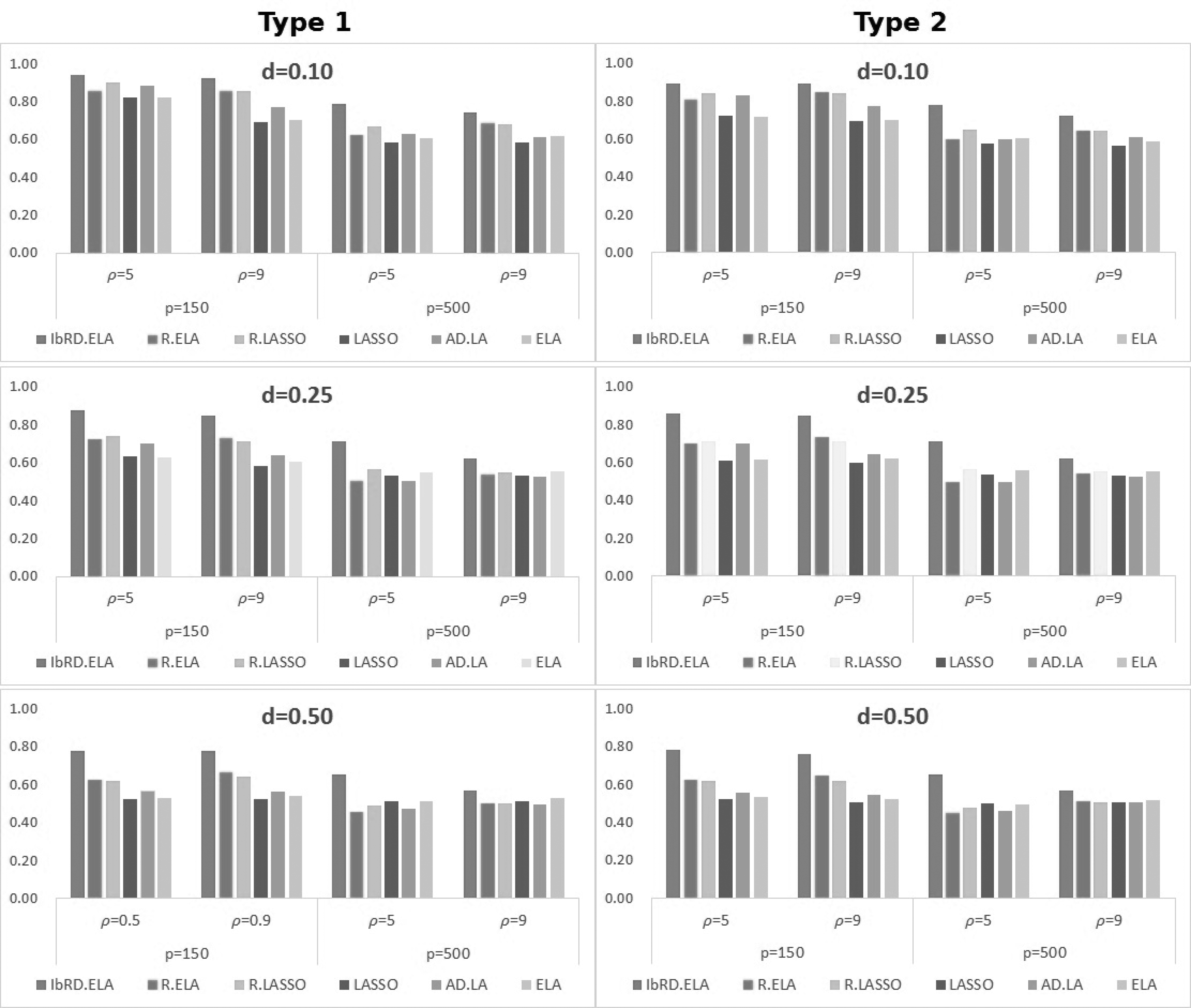
\end{document}. The procedures for generating artificial data sets are given in Figure 2. We consider training set and test set with sample size 100 and 20, respectively.
Processes of generating data set for simulation studies.
We make a comparison between the proposed method (IbRD.ELA) with existing methods: random elastic net (R.ELA) and random lasso (R.LASSO). The performances of the ordinary lasso (LASSO), adaptive lasso (AD.LA), and elastic net (ELA) are also compared. We consider the number of bootstrap samples to \documentclass{aastex}\usepackage{amsbsy}\usepackage{amsfonts}\usepackage{amssymb}\usepackage{bm}\usepackage{mathrsfs}\usepackage{pifont}\usepackage{stmaryrd}\usepackage{textcomp}\usepackage{portland, xspace}\usepackage{amsmath, amsxtra}\pagestyle{empty}\DeclareMathSizes{10}{9}{7}{6}\begin{document}
$$B = 500$$
\end{document} and the range of weight \documentclass{aastex}\usepackage{amsbsy}\usepackage{amsfonts}\usepackage{amssymb}\usepackage{bm}\usepackage{mathrsfs}\usepackage{pifont}\usepackage{stmaryrd}\usepackage{textcomp}\usepackage{portland, xspace}\usepackage{amsmath, amsxtra}\pagestyle{empty}\DeclareMathSizes{10}{9}{7}{6}\begin{document}
$$[ L,U ]$$
\end{document} as \documentclass{aastex}\usepackage{amsbsy}\usepackage{amsfonts}\usepackage{amssymb}\usepackage{bm}\usepackage{mathrsfs}\usepackage{pifont}\usepackage{stmaryrd}\usepackage{textcomp}\usepackage{portland, xspace}\usepackage{amsmath, amsxtra}\pagestyle{empty}\DeclareMathSizes{10}{9}{7}{6}\begin{document}
$$[ 0.5 , 1.5 ]$$
\end{document}. In the L1-type regularized regression modeling, the tuning parameters are selected by the five-fold cross-validation. We show the root mean squared error as a prediction accuracy and the average of true positive (i.e., TP: average number of the truly nonzero coefficients, incorrectly set to zero) and true negative (i.e., TN: the average percentage of true zero coefficients, which were correctly set to 0) rates as a variable selection result.
Table 1 shows the prediction accuracy for the methods. We can see through Table 1 that the proposed IbRD.ELA shows the outstanding performances in all simulation situations. Although the existing random lasso-type approaches (i.e., random elastic net and random lasso) cannot always show the effective performances, the proposed IbRD.ELA shows superiority in the viewpoint of the prediction accuracy. It implies that incorporating the knowledge about data sets may lead to effective modeling results.
Results of Prediction Errors in the Monte Carlo Simulations
AD.LA, adaptive lasso; ELA, elastic net; LASSO, ordinary lasso; IbRD.ELA, interaction-based random elastic net; R.ELA, random elastic net; R.LASSO, random lasso.
Figure 3 shows the variable selection results given as an average of TP and TN rates. The proposed method also shows effective performances in variable selection. The outstanding performances of our method can also be seen in the presence of multicollinearity (i.e., \documentclass{aastex}\usepackage{amsbsy}\usepackage{amsfonts}\usepackage{amssymb}\usepackage{bm}\usepackage{mathrsfs}\usepackage{pifont}\usepackage{stmaryrd}\usepackage{textcomp}\usepackage{portland, xspace}\usepackage{amsmath, amsxtra}\pagestyle{empty}\DeclareMathSizes{10}{9}{7}{6}\begin{document}
$$\rho = 0.9$$
\end{document}). We can also see that the random lasso-type approaches (i.e., IbRD.ELA, RD.ELA, and RD.LASSO) outperform variable selection compared with the existing lasso, adaptive lasso, and elastic net. It implies that the use of the random forest method in bootstrap regression modeling may lead to effective feature selection by overcoming the multicollinearity between predictors.
Variable selection results: average of true positive and true negative rates. AD.LA, adaptive lasso; ELA, elastic net; LASSO, ordinary lasso; R.ELA, random elastic net; R.LASSO, random lasso.
The results for prediction accuracy and variable selection imply that the proposed method incorporating the interaction of features is an effective tool for linear regression modeling when interaction of features is a crucial symptom of a phenomenon.
4. Driver Gene Selection Through Copy Number-Driven Expression Levels Through TCGA Data Analysis
We apply the proposed interaction-based random elastic net (IbRD.ELA) to cancer driver gene selection through TCGA project data set. The TCGA data set consists of comprehensive genome scale information, for example, expression levels, copy number alterations, and mutation status. We consider the following cancer data sets: lung squamous cell carcinoma (LUSC), cervical cancer (CESC), glioblastoma multiforme (GBM), prostate adenocarcinoma (PRAD), ovarian serous cystadenocarcinoma (OV), papillary kidney carcinoma (KIRP), lower grade glioma (LGG), and head and neck squamous cell carcinoma (HNSC) from TCGA data set.
To identify the cancer driver genes, we first extract gene expression modules from expression levels of genes by using extraction of expression module (EEM) (Niida et al., 2009), and consider the extracted modules as response variables in regression modeling. For details on the EEMs, see Niida et al. (2009). We extract 7, 9, 8, 9, 8, 9, 8, and 9 modules from expression levels of LUSC, CESC, GBM, PRAD, OV, KIRP, LGG, and HNSC data set, respectively. In other words, we consider 7, 9, 8, 9, 8, 9, 8, and 9 response variables (i.e., 7, 9, 8, 9, 8, 9, 8, and 9 regression models) for each cancer. The data sets for LUSC, CESC, GBM, PRAD, OV, KIRP, LGG, and HNSC consist of 401, 111, 136, 175, 257, 103, and 299 samples, respectively. We choose to use 80% for the training set and the rest 20% as the test set. And, the expression levels for \documentclass{aastex}\usepackage{amsbsy}\usepackage{amsfonts}\usepackage{amssymb}\usepackage{bm}\usepackage{mathrsfs}\usepackage{pifont}\usepackage{stmaryrd}\usepackage{textcomp}\usepackage{portland, xspace}\usepackage{amsmath, amsxtra}\pagestyle{empty}\DeclareMathSizes{10}{9}{7}{6}\begin{document}
$$p = 500$$
\end{document} genes that have the highest variance of expression levels in all samples are considered as predictor variables for each cancer data analysis.
In TCGA data analysis, we consider additional scores taking the \documentclass{aastex}\usepackage{amsbsy}\usepackage{amsfonts}\usepackage{amssymb}\usepackage{bm}\usepackage{mathrsfs}\usepackage{pifont}\usepackage{stmaryrd}\usepackage{textcomp}\usepackage{portland, xspace}\usepackage{amsmath, amsxtra}\pagestyle{empty}\DeclareMathSizes{10}{9}{7}{6}\begin{document}
$$cis -$$
\end{document} effect and the \documentclass{aastex}\usepackage{amsbsy}\usepackage{amsfonts}\usepackage{amssymb}\usepackage{bm}\usepackage{mathrsfs}\usepackage{pifont}\usepackage{stmaryrd}\usepackage{textcomp}\usepackage{portland, xspace}\usepackage{amsmath, amsxtra}\pagestyle{empty}\DeclareMathSizes{10}{9}{7}{6}\begin{document}
$$trans -$$
\end{document} effect of copy number alterations on expression levels based on the following residual:
\documentclass{aastex}\usepackage{amsbsy}\usepackage{amsfonts}\usepackage{amssymb}\usepackage{bm}\usepackage{mathrsfs}\usepackage{pifont}\usepackage{stmaryrd}\usepackage{textcomp}\usepackage{portland, xspace}\usepackage{amsmath, amsxtra}\pagestyle{empty}\DeclareMathSizes{10}{9}{7}{6}\begin{document}
\begin{align*}
{\textbf{\textit{ x}}_k} = {\textbf{\textit{ z}}_k}{ \hat { \gamma}_k} + \,{ \bm{\varepsilon}^{\prime\prime}_k}, \tag{18}
\end{align*}
\end{document}
Like Ib.ELA based on both effects (Ib.ELA(B)) in (9), we also consider Ib.ELA based on \documentclass{aastex}\usepackage{amsbsy}\usepackage{amsfonts}\usepackage{amssymb}\usepackage{bm}\usepackage{mathrsfs}\usepackage{pifont}\usepackage{stmaryrd}\usepackage{textcomp}\usepackage{portland, xspace}\usepackage{amsmath, amsxtra}\pagestyle{empty}\DeclareMathSizes{10}{9}{7}{6}\begin{document}
$$cis -$$
\end{document} effect and \documentclass{aastex}\usepackage{amsbsy}\usepackage{amsfonts}\usepackage{amssymb}\usepackage{bm}\usepackage{mathrsfs}\usepackage{pifont}\usepackage{stmaryrd}\usepackage{textcomp}\usepackage{portland, xspace}\usepackage{amsmath, amsxtra}\pagestyle{empty}\DeclareMathSizes{10}{9}{7}{6}\begin{document}
$$trans -$$
\end{document} effect as follows.
where
\documentclass{aastex}\usepackage{amsbsy}\usepackage{amsfonts}\usepackage{amssymb}\usepackage{bm}\usepackage{mathrsfs}\usepackage{pifont}\usepackage{stmaryrd}\usepackage{textcomp}\usepackage{portland, xspace}\usepackage{amsmath, amsxtra}\pagestyle{empty}\DeclareMathSizes{10}{9}{7}{6}\begin{document}
\begin{align*}
w_j^t = 1 \bigg/ \left( \frac { 1 } { U } + { \frac { \big[ \{
Score_j^ { trans - } - min ( Score_j^ { trans - } ) \} ( \frac { 1
} { L } - \frac { 1 } { U } ) \big] } { { \rm { max } } (
Score_j^ { trans - } ) - { \rm { min } } ( Score_j^ { trans - } )
} } \right). \tag { 24 }
\end{align*}
\end{document}
We apply Ib.ELA(C) and Ib.ELA(T) to random lasso procedures, similar to IbRD.ELA(B). We then perform uncovering cancer driver genes based on IbRD.ELA(B), IbRD.ELA(C), and IbRD.ELA(T)). The tuning parameters \documentclass{aastex}\usepackage{amsbsy}\usepackage{amsfonts}\usepackage{amssymb}\usepackage{bm}\usepackage{mathrsfs}\usepackage{pifont}\usepackage{stmaryrd}\usepackage{textcomp}\usepackage{portland, xspace}\usepackage{amsmath, amsxtra}\pagestyle{empty}\DeclareMathSizes{10}{9}{7}{6}\begin{document}
$$\lambda$$
\end{document} and \documentclass{aastex}\usepackage{amsbsy}\usepackage{amsfonts}\usepackage{amssymb}\usepackage{bm}\usepackage{mathrsfs}\usepackage{pifont}\usepackage{stmaryrd}\usepackage{textcomp}\usepackage{portland, xspace}\usepackage{amsmath, amsxtra}\pagestyle{empty}\DeclareMathSizes{10}{9}{7}{6}\begin{document}
$$\alpha$$
\end{document} in the L1-type regularized regression modeling are selected by five-fold cross-validation, and we consider the number of bootstrap samples on random lasso procedure to \documentclass{aastex}\usepackage{amsbsy}\usepackage{amsfonts}\usepackage{amssymb}\usepackage{bm}\usepackage{mathrsfs}\usepackage{pifont}\usepackage{stmaryrd}\usepackage{textcomp}\usepackage{portland, xspace}\usepackage{amsmath, amsxtra}\pagestyle{empty}\DeclareMathSizes{10}{9}{7}{6}\begin{document}
$$B = 500$$
\end{document} and the range of weight \documentclass{aastex}\usepackage{amsbsy}\usepackage{amsfonts}\usepackage{amssymb}\usepackage{bm}\usepackage{mathrsfs}\usepackage{pifont}\usepackage{stmaryrd}\usepackage{textcomp}\usepackage{portland, xspace}\usepackage{amsmath, amsxtra}\pagestyle{empty}\DeclareMathSizes{10}{9}{7}{6}\begin{document}
$$[ L,U ]$$
\end{document} as \documentclass{aastex}\usepackage{amsbsy}\usepackage{amsfonts}\usepackage{amssymb}\usepackage{bm}\usepackage{mathrsfs}\usepackage{pifont}\usepackage{stmaryrd}\usepackage{textcomp}\usepackage{portland, xspace}\usepackage{amsmath, amsxtra}\pagestyle{empty}\DeclareMathSizes{10}{9}{7}{6}\begin{document}
$$[ 0.5 , \,1.5 ]$$
\end{document}.
Table 2 shows the average of root mean squared errors of 7, 9, 8, 9, 8, 9, 8, and 9 regression models for each LUSC, CESC, GBM, PRAD, OV, KIRP, LGG, and HNSC, respectively. We can see through the results that the proposed IbRD.ELA(B) shows outstanding performances in the viewpoint of prediction accuracy. It can also be seen that the random lasso-type approaches (i.e., IbRD.ELA(B), IbRD.ELA(C), IbRD.ELA(T), R.ELA, and R.LASSO) perform well compared with the ordinary L1-type approaches (i.e., LASSO, AD.LA, and ELA) overall. It implies that the random forest method in bootstrap regression modeling may provide effective performances for regression modeling by overcoming the demerits caused from multicollinearity. Furthermore, we can see that the proposed interaction-based feature-selection approaches, that is, IbRD.ELA(B), IbRD.ELA(C), and IbRD.ELA(T), outperform regression modeling compared with the existing L1-type regularization methods. These results imply that incorporating the biological knowledge (i.e., a crucial symptom of tumor pathogenesis: influence of copy number alterations on expression levels) may lead to effective results in uncovering cancer driver gene, and thus the proposed methods provide outstanding results in prediction accuracy.
Average of Prediction Error in the Cancer Genome Atlas Data Analysis
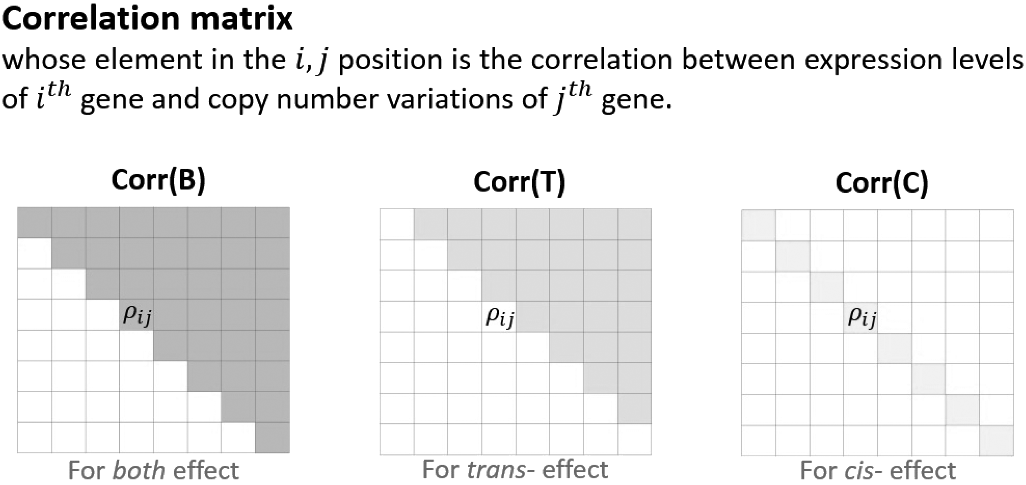
We also show the correlation between expression levels and copy number alterations of selected and deleted genes by the proposed methods IbRD.ELA(B), IbRD.ELA(C), IbRD.ELA(T), and ordinary random elastic net. Table 3 shows averages of correlations between the expression levels and copy number alterations of selected (Y) and deleted genes (N). To show the correlation in line with the both (Corr(B)), \documentclass{aastex}\usepackage{amsbsy}\usepackage{amsfonts}\usepackage{amssymb}\usepackage{bm}\usepackage{mathrsfs}\usepackage{pifont}\usepackage{stmaryrd}\usepackage{textcomp}\usepackage{portland, xspace}\usepackage{amsmath, amsxtra}\pagestyle{empty}\DeclareMathSizes{10}{9}{7}{6}\begin{document}
$$trans -$$
\end{document} (Corr(T)) and \documentclass{aastex}\usepackage{amsbsy}\usepackage{amsfonts}\usepackage{amssymb}\usepackage{bm}\usepackage{mathrsfs}\usepackage{pifont}\usepackage{stmaryrd}\usepackage{textcomp}\usepackage{portland, xspace}\usepackage{amsmath, amsxtra}\pagestyle{empty}\DeclareMathSizes{10}{9}{7}{6}\begin{document}
$$cis -$$
\end{document} (Corr(C)) effects, we compute the average of elements in the upper triangular correlation matrix with diagonal, the upper triangular correlation matrix without diagonal, and elements in diagonal of the correlation matrix, respectively. In other words, the averages of correlation in line with both\documentclass{aastex}\usepackage{amsbsy}\usepackage{amsfonts}\usepackage{amssymb}\usepackage{bm}\usepackage{mathrsfs}\usepackage{pifont}\usepackage{stmaryrd}\usepackage{textcomp}\usepackage{portland, xspace}\usepackage{amsmath, amsxtra}\pagestyle{empty}\DeclareMathSizes{10}{9}{7}{6}\begin{document}
$$trans -$$
\end{document} and \documentclass{aastex}\usepackage{amsbsy}\usepackage{amsfonts}\usepackage{amssymb}\usepackage{bm}\usepackage{mathrsfs}\usepackage{pifont}\usepackage{stmaryrd}\usepackage{textcomp}\usepackage{portland, xspace}\usepackage{amsmath, amsxtra}\pagestyle{empty}\DeclareMathSizes{10}{9}{7}{6}\begin{document}
$$cis -$$
\end{document} effects are computed based on the elements in the correlation matrix tones of dark, middle, and light grey in Figure 4, respectively. It can be seen through Table 3 that the two factors of the selected genes are highly correlated compared with the two factors of the deleted genes. It implies that the two factors of the crucial genes for explaining the variations of expression modules are highly correlated. It can also be seen that the genes selected (deleted) by IbRD.ELA(B) and IbRD.ELA(C) show higher (lower) correlation than the genes selected by R.ELA given in rows Corr (B) and Corr(C). However, the genes selected by IbRD.ELA(T) cannot show the strong correlation between the two factors. From these results, we can see that the proposed methods IbRD.ELA(B) and IbRD.ELA(C) tend to select genes having strong correlation between the expression levels and copy number alterations. In short, the proposed methods (i.e., IbRD.ELA(B) and IbRD.ELA(C)) perform effectively uncovering cancer driver gene by incorporating the symptom of cancer: the influence of copy number alterations on expression levels.
Correlation in line with both\documentclass{aastex}\usepackage{amsbsy}\usepackage{amsfonts}\usepackage{amssymb}\usepackage{bm}\usepackage{mathrsfs}\usepackage{pifont}\usepackage{stmaryrd}\usepackage{textcomp}\usepackage{portland, xspace}\usepackage{amsmath, amsxtra}\pagestyle{empty}\DeclareMathSizes{10}{9}{7}{6}\begin{document}
$$cis -$$
\end{document} and \documentclass{aastex}\usepackage{amsbsy}\usepackage{amsfonts}\usepackage{amssymb}\usepackage{bm}\usepackage{mathrsfs}\usepackage{pifont}\usepackage{stmaryrd}\usepackage{textcomp}\usepackage{portland, xspace}\usepackage{amsmath, amsxtra}\pagestyle{empty}\DeclareMathSizes{10}{9}{7}{6}\begin{document}
$$trans -$$
\end{document} effects.
Correlation Between Expression Levels and Copy Number Alterations
IbRD.ELA(B)
IbRD.ELA(T)
IbRD.ELA(C)
R.ELA
N
Y
N
Y
N
Y
N
Y
LUSC
Corr(B)
0.072
0.083
0.076
0.076
0.074
0.081
0.074
0.079
Corr(T)
0.072
0.083
0.075
0.075
0.073
0.080
0.074
0.078
Corr(C)
0.106
0.123
0.110
0.116
0.102
0.132
0.110
0.116
CESC
Corr(B)
0.103
0.106
0.103
0.103
0.102
0.106
0.103
0.102
Corr(T)
0.102
0.106
0.103
0.102
0.102
0.105
0.103
0.101
Corr(C)
0.126
0.139
0.128
0.133
0.112
0.183
0.129
0.136
GBM
Corr(B)
0.092
0.104
0.095
0.095
0.094
0.099
0.095
0.096
Corr(T)
0.091
0.104
0.095
0.095
0.094
0.098
0.095
0.096
Corr(C)
0.113
0.136
0.116
0.128
0.110
0.147
0.120
0.118
PRAD
Corr(B)
0.077
0.087
0.079
0.080
0.078
0.084
0.079
0.081
Corr(T)
0.077
0.086
0.079
0.080
0.078
0.083
0.079
0.081
Corr(C)
0.092
0.103
0.095
0.096
0.084
0.124
0.096
0.093
OV
Corr(B)
0.073
0.078
0.074
0.075
0.073
0.078
0.074
0.076
Corr(T)
0.073
0.077
0.074
0.074
0.073
0.076
0.074
0.075
Corr(C)
0.147
0.160
0.150
0.155
0.136
0.186
0.152
0.149
KIRP
Corr(B)
0.132
0.140
0.136
0.129
0.131
0.143
0.135
0.131
Corr(T)
0.132
0.140
0.136
0.129
0.131
0.143
0.135
0.130
Corr(C)
0.134
0.148
0.138
0.137
0.123
0.178
0.137
0.140
LGG
Corr(B)
0.099
0.138
0.105
0.116
0.100
0.136
0.105
0.118
Corr(T)
0.099
0.137
0.105
0.115
0.100
0.135
0.105
0.118
Corr(C)
0.108
0.148
0.113
0.135
0.101
0.174
0.115
0.131
HNSC
Corr(B)
0.079
0.100
0.083
0.090
0.080
0.096
0.082
0.095
Corr(T)
0.079
0.099
0.082
0.089
0.080
0.096
0.081
0.094
Corr(C)
0.111
0.142
0.115
0.132
0.107
0.152
0.116
0.133
To demonstrate a reliability of the proposed methods and biological evidence of the identified genes, we show the selected genes for each cancer and their evidence. Table 4 shows the selected genes in all 7, 9, 8, 9, 8, 9, 8, and 9 regression models for each cancer, that is, LUSC, CESC, GBM, PRAD, OV, KIRP, LGG, and HNSC, respectively. The “B”, “T,” and “C” in column “Effect” indicate that the genes are selected by IbRD.ELA based on both\documentclass{aastex}\usepackage{amsbsy}\usepackage{amsfonts}\usepackage{amssymb}\usepackage{bm}\usepackage{mathrsfs}\usepackage{pifont}\usepackage{stmaryrd}\usepackage{textcomp}\usepackage{portland, xspace}\usepackage{amsmath, amsxtra}\pagestyle{empty}\DeclareMathSizes{10}{9}{7}{6}\begin{document}
$$trans -$$
\end{document} and \documentclass{aastex}\usepackage{amsbsy}\usepackage{amsfonts}\usepackage{amssymb}\usepackage{bm}\usepackage{mathrsfs}\usepackage{pifont}\usepackage{stmaryrd}\usepackage{textcomp}\usepackage{portland, xspace}\usepackage{amsmath, amsxtra}\pagestyle{empty}\DeclareMathSizes{10}{9}{7}{6}\begin{document}
$$cis -$$
\end{document} effects, respectively.
It can be first seen from Table 4 that the uncovered genes have strong biological evidence as a cancer driver gene given as columns “Evidence” and “Cancer”. We can also see that the identified genes by IbRD.ELA based on \documentclass{aastex}\usepackage{amsbsy}\usepackage{amsfonts}\usepackage{amssymb}\usepackage{bm}\usepackage{mathrsfs}\usepackage{pifont}\usepackage{stmaryrd}\usepackage{textcomp}\usepackage{portland, xspace}\usepackage{amsmath, amsxtra}\pagestyle{empty}\DeclareMathSizes{10}{9}{7}{6}\begin{document}
$$cis -$$
\end{document} effect have relatively strong evidence. We focus on the genes leucine-rich repeat containing G protein coupled receptor 5 (LGR5), sortilin-related VPS10 domain containing receptor 2 (SORCS2), and transgelin 3 (TAGLN3), which are selected by more than one method in a cancer data analysis (i.e., LGR5 is selected by IbRD.ELA(B), IbRD.ELA(T), and IbRD.ELA(C) in analysis of LUSC data set; TAGLN3 and SORCS2 are selected by IbRD.ELA(B) and IbRD.ELA(C) in analysis of KIRP data set). In other words, the genes can be considered as a driver gene to explain the corresponding cancer pathogenesis processes. The LGR5 was known as a candidate marker of nonsmall cell lung cancer, and positive LGR5 expression was defined in 28.4% of nonsmall cell lung cancer tumors (Gao et al., 2015). Furthermore, LGR5 expression level was upregulated in primary colorectal carcinomas samples compared with normal colorectal epithelium (Hirsch et al., 2014). The SORCS2 gene expression level was strongly related to sensitivity to chemotherapeutics in human gastric cancer cell lines, and the protein expression of SORCS2 is related to sensitivity to chemotherapeutics in human gastric cancer cell lines (Wu et al., 2011). TAGLN3, which is a microtubule-associated protein, was strongly expressed in the ventral diencephalon (Ratie et al., 2013). Furthermore, Ratie et al. (2013) demonstrated that TAGLN3 was upregulated in the olfactory placodes, the ventral diencephalon, the mesencephalic roof, the ganglions, and the neural tube.
These results imply that our methods provide reliable results for cancer driver gene selection. In short, the proposed methods incorporating biological knowledge will be a useful tool for uncovering cancer driver gene.
5. Conclusions
We have introduced the statistical strategies to identify cancer driver genes. To perform effective and interpretable gene selection, we have considered incorporation of the biological knowledge to feature-selection procedures. In other words, we have incorporated an association of the expression levels and copy number alterations, which was well known as a crucial phenomenon of oncogenes, into gene-selection procedures based on the adaptive elastic net. Then, we have proposed the interaction-based random elastic net in line with the random lasso procedure.
Monte Carlo simulations and TCGA data analysis showed that the proposed strategies outperform for variable selection and prediction accuracy. Furthermore, we have observed through the TCGA data analysis that the proposed methods provide reliable results in gene selection. We expect that the proposed strategies will be useful tools for high-dimensional genomic data analysis, especially driver gene selection. Although we have described that the proposed methods focused on the driver gene selection, the incorporation of the knowledge of data sets leads to effective and interpretable analysis results. Thus, we expect that the proposed methods can perform effectively feature selection in various fields of research.
We have used the weight to control the amount of L1-type penalty in line with the adaptive L1-type penalty. To prevent that the weight excessively dominates an amount of L1-type penalty (i.e., feature-selection procedures), we have considered the range of the weight wk between L and U. However, the range was arbitrarily decided in numerical studies (i.e., \documentclass{aastex}\usepackage{amsbsy}\usepackage{amsfonts}\usepackage{amssymb}\usepackage{bm}\usepackage{mathrsfs}\usepackage{pifont}\usepackage{stmaryrd}\usepackage{textcomp}\usepackage{portland, xspace}\usepackage{amsmath, amsxtra}\pagestyle{empty}\DeclareMathSizes{10}{9}{7}{6}\begin{document}
$$L = 0.5$$
\end{document} and \documentclass{aastex}\usepackage{amsbsy}\usepackage{amsfonts}\usepackage{amssymb}\usepackage{bm}\usepackage{mathrsfs}\usepackage{pifont}\usepackage{stmaryrd}\usepackage{textcomp}\usepackage{portland, xspace}\usepackage{amsmath, amsxtra}\pagestyle{empty}\DeclareMathSizes{10}{9}{7}{6}\begin{document}
$$U = 1.5$$
\end{document}) even though the amount of the weight is crucial in interaction-based feature selection. To improve the feature-selection procedures, further work remains to be done in consideration of the range as a tuning parameter and the parameter selection based on model selection criteria.
Footnotes
Author Disclosure Statement
No competing financial interests exist.
References
1.
AlgamalZ.Y., and LeeM.H.2015. Penalized logistic regression with the adaptive LASSO for gene selection in high-dimensional cancer classification. Exp. Syst. Appl., 42, 9326–9332
2.
ChangH.J., YangM.J., YangY.H., et al.2009. MMP13 is potentially a new tumor marker for breast cancer diagnosis. Oncol. Rep. 22, 1119–1127.
3.
DasJ., GayvertK.M., BuneaF., et al.2015. ENCAPP: Elastic-net-based prognosis prediction and biomarker discovery for human cancers. BMC Genomics, 16, 263.
4.
DavoliT., XuA.W., MengwasserK.E., et al.2013. Cumulative haploinsufficiency and triplosensitivity drive aneuploidy patterns and shape the cancer genome. Cell, 155, 948–962.
5.
GaoF., ZhouB., XuJ.C., et al.2015. The role of LGR5 and ALDH1A1 in non-small cell lung cancer: Cancer progression and prognosis. Biochem. Biophys. Res. Commun., 462, 91–98.
6.
GhoshD., and ChinnaiyanA.M.2005. Classification and selection of biomarkers in genomic data using lasso. J. Biomed. Biotechnol., 2005, 147–154.
7.
HirschD., BarkerN., McNeilN., et al.2014. LGR5 positivity defines stem-like cells in colorectal cancer. Carcinogenesis, 35, 849–858.
8.
HensJ.R., and WysolmerskiJ.J.2005. Key stages of mammary gland development: Molecular mechanisms involved in the formation of the embryonic mammary gland. Breast Cancer Res. 7, 220–224.
9.
KangM., QinW., BuyaM., et al.2016. VNN1, a potential biomarker for pancreatic cancer-associated new-onset diabetes, aggravates paraneoplastic islet dysfunction by increasing oxidative stress. Cancer Lett. 373, 241–250.
10.
KornumB.R., KawashimaM., FaracoJ., et al.2011. Common variants in P2RY11 are associated with narcolepsy. Nat. Genet., 43, 66–71.
11.
LeisO., EguiaraA., Lopez-ArribillagaE., et al.2012. Sox2 expression in breast tumours and activation in breast cancer stem cells. Oncogene, 31, 1354–1365.
12.
LinD., ZhangJ., LiJ., et al.2013. Group sparse canonical correlation analysis for genomic data integration. BMC Bioinformatics. 14, 245.
13.
LinW., WatanabeH., PengS., et al.2015. Dynamic epigenetic regulation by menin during pancreatic islet tumor formation. Mol. Cancer. Res., 13, 689–698.
14.
LipsonD., Ben-DorA., DehanE., et al.2004. Joint analysis of DNA copy numbers and gene expression levels. In: JonassenI., and KimJ. (eds.). Proc. Algor. Bioinf. WABI, 2004. Vol. 3240, pp 135–146. Bergen, Norway.
15.
LugerD., YangY.A., RavivA., et al.2013. Expression of the B-cell receptor component CD79a on immature myeloid cells contributes to their tumor promoting effects. PLoS One, 8:e76115.
16.
McWilliamsR.R., WiebenE.D., RabeK.G., et al.2011. Prevalence of CDKN2A mutations in pancreatic cancer patients: Implications for genetic counseling. Eur. J. Hum. Genet., 19, 472–478.
17.
MoM.L., OkamotoJ., ChenZ., et al.2013. Down-regulation of SIX3 is associated with clinical outcome in lung adenocarcinoma. PLoS One, 8:e71816.
18.
MonneratC., ChompretA., KannengiesserC., et al.2007. BRCA1, BRCA2, TP53, and CDKN2A germline mutations in patients with breast cancer and cutaneous melanoma. Fam. Cancer, 6, 453–461.
19.
MorganE. K, annan-ThulasiramanP., and NoyN.2010. Involvement of fatty acid binding protein 5 and PPARbeta/\documentclass{aastex}\usepackage{amsbsy}\usepackage{amsfonts}\usepackage{amssymb}\usepackage{bm}\usepackage{mathrsfs}\usepackage{pifont}\usepackage{stmaryrd}\usepackage{textcomp}\usepackage{portland, xspace}\usepackage{amsmath, amsxtra}\pagestyle{empty}\DeclareMathSizes{10}{9}{7}{6}\begin{document}$$\delta$$\end{document}in prostate cancer cell growth. PPAR Res. 2010, 234629.
20.
NiidaA., SmithA.D., ImotoS., et al.2009. Gene set-based module discovery in the breast cancer transcriptome. BMC Bioinformatics, 10, 71.
21.
OhmachiT., InoueH., MimoriK., et al.2006. Fatty acid binding protein 6 is overexpressed in colorectal cancer. Clin. Cancer Res., 12, 5090–5095.
22.
ParkH., ImotoS., and MiyanoS.2015. Recursive random lasso for identifying anti-cancer drug targets. PLoS One, 10, e0141869.
23.
PowellC.A., NasserM.W., ZhaoH., et al.2015. Fatty acid binding protein 5 promotes metastatic potential of triple negative breast cancer cells through enhancing epidermal growth factor receptor stability. Oncotarget, 6, 6373–6385.
24.
RatieL., WareM., Barloy-Hubler, et al.2013. Novel genes upregulated when NOTCH signalling is disrupted during hypothalamic development. Neural Dev. 8, 25.
25.
SimovichM.J., MillerB., EzzeldinH., et al.2001. Four novel mutations in the RPE65 gene in patients with Leber congenital amaurosis. Hum. Mutat. 18, 164.
26.
TibshiraniR.1996. Regression shrinkage and selection via the lasso. J. Roy. Stat. Soc. Ser. B, 73, 273–282.
27.
TengB.P., HefflerM.D., LaiE.C., et al.2011. Inhibition of hyaluronan synthase-3 decreases subcutaneous colon cancer growth by increasing apoptosis. Anticancer Agents Med. Chem., 11, 620–628.
28.
VoldborgB.R., DamstrupL., Spang-ThomsenM., et al.1997. Epidermal growth factor receptor (EGFR) and EGFR mutations, function and possible role in clinical trials. Ann. Oncol., 8, 1197–1206.
29.
WaldmannP., MeszarosG., GredlerB., et al.2013. Evaluation of the lasso and the elastic net in genome-wide association studies. Front. Genet. 4, 270.
30.
WangS., NamB., RossetS., et al.2011. Random lasso. Ann. Appl. Stat., 5, 468–485.
31.
WellsW.A., SchwartzG.N., MorganelliP.M., et al.2006. Expression of “Spot 14” (THRSP) predicts disease free survival in invasive breast cancer: Immunohistochemical analysis of a new molecular marker. Breast Cancer Res. Treat., 98, 231–240.
32.
WhitneyD.H., ElashoffM.R., Porta-SmithK., et al.2015. Derivation of a bronchial genomic classifier for lung cancer in a prospective study of patients undergoing diagnostic bronchoscopy. BMC Med Genomics, 8, 18.
33.
WuF., YeX., WangP., et al.2013. Sox2 suppresses the invasiveness of breast cancer cells via a mechanism that is dependent on Twist1 and the status of Sox2 transcription activity. BMC Cancer, 13, 317.
34.
WuX., YeY., RosellR., et al.2011. Genome-wide association study of survival in non-small cell lung cancer patients receiving platinum-based chemotherapy. J. Natl. Cancer Inst., 103, 817–825.
35.
YamadaT., OshimaT., YoshiharaK., et al.2010. Overexpression of MMP-13 gene in colorectal cancer with liver metastasis. Anticancer Res. 30, 2693–2699.
36.
YanL.X., WuQ.N., ZhangY., et al.2011. Knockdown of miR-21 in human breast cancer cell lines inhibits proliferation, in vitro migration and in vivo tumor growth. Breast Cancer Res. 13:R2.
37.
YangL., TangH., KongY., et al.2015. LGR5 promotes breast cancer progression and maintains stem-like cells through activation of Wnt/β-catenin signaling. Stem Cells, 33, 2913–2924.
38.
YuX.J., YangM.J., ZhouB., et al.2015. Characterization of somatic mutations in air pollution-related lung cancer. EBioMedicine, 2, 583–590.
39.
YuanY., CurtisC., CaldasC., et al.2012. A sparse regulatory network of copy-number driven gene expression reveals putative breast cancer oncogenes. IEEE/ACM Trans. Comput. Biol. Bioinform., 9, 947–954.
40.
ZouH.2006. The adaptive lasso and its oracle properties. J. Am. Stat. Assoc., 101, 1418–1429.
41.
ZouH., and HastieT.2008. Regularization and variable selection via the elastic net. J. R. Stat. Soc. Ser. B, 6, 301–320.