Safe and Complete Contig Assembly Through Omnitigs *

Abstract

Contig assembly is the first stage that most assemblers solve when reconstructing a genome from a set of reads. Its output consists of contigs—a set of strings that are promised to appear in any genome that could have generated the reads. From the introduction of contigs 20 years ago, assemblers have tried to obtain longer and longer contigs, but the following question remains: given a genome graph G (e.g., a de Bruijn, or a string graph), what are all the strings that can be safely reported from G as contigs? In this article, we answer this question using a model in which the genome is a circular covering walk. We also give a polynomial-time algorithm to find such strings, which we call omnitigs. Our experiments show that omnitigs are 66%–82% longer on average than the popular unitigs, and 29% of dbSNP locations have more neighbors in omnitigs than in unitigs.

1. Introduction

The genome assembly problem is to reconstruct the sequence of a genome using reads from a sequencing experiment. It is one of the oldest bioinformatics problems; nevertheless, recent projects such as the Genome 10K have underscored the need to further improve assemblers (Haussler et al., 2008). Current algorithms face numerous practical challenges, including scalability, integration of new data types (e.g., PacBio), and representation of multiple alleles. Although handling these challenges is extremely important, assemblers do not produce optimal results even in very simple and idealized scenarios. To address this, several articles have developed better theoretical underpinnings (Idury and Waterman, 1995; Myers, 2005; Medvedev et al., 2007, 2011; Simpson and Durbin, 2010; Vyahhi et al., 2012), often resulting in improved assemblers in practice (Pevzner et al., 2001; Zerbino and Birney, 2008; Simpson and Durbin, 2011; Bankevich et al., 2012).

In most theoretical studies, the assembly problem is formulated as finding one genomic reconstruction, that is, a single string that represents the sequence of the genome. However, the presence of repeats means that a unique genomic reconstruction usually does not exist. In practice, assemblers instead output several strings, called contigs, which are “promised” to occur in the genome. We refer to this restatement of the genome assembly problem as contig assembly. Contigs can then be used to answer biological questions (e.g., about gene content) or perform comparative genomic analysis. When mate pairs are available, contigs can be fed to later assembly stages, such as scaffolding (Boetzer et al., 2011; Luo et al., 2012; Sahlin et al., 2014) and then gap filling (Boetzer and Pirovano, 2012; Salmela et al., 2015).

Assemblers implement different strategies for finding contigs. The common strategy is to find unitigs, an idea that can be traced back to Kececioglu and Myers (1995). Unitigs have the desired property that they can be mathematically proven to occur in all possible genomic reconstructions, under clear assumptions on what “genomic reconstruction” means. We will refer to strings that satisfy such a property as being safe (Definition 3), and will say that a contig assembly algorithm is safe if it outputs only safe strings. Although most assemblers have a safe strategy at their core, they also incorporate heuristics to handle erroneous data and extend contig length (e.g., bubble popping, tip removal, and path disambiguation). Properties of such heuristics, however, are difficult to prove, and this article focuses on core algorithms that are safe.

Although the unitig algorithm is safe, it does not identify all possible safe strings (see Fig. 2). An improved safe algorithm was used in the EULER assembler (Pevzner et al., 2001), and further improvements were suggested based on iteratively simplifying the graph used for assembly (Pevzner et al., 2001; Jackson, 2009; Medvedev and Brudno, 2009; Kingsford et al., 2010). However, we show that these algorithms still do not always output all the safe strings. In fact, since the initial consideration of contig assembly 20 years ago, the fundamental question of finding all the safe strings of a graph remains poorly studied.

In this article, we answer this question by giving a polynomial-time algorithm for outputting all the safe strings in the common genome graph models (de Bruijn and string graphs) when the genome is a circular covering walk (Section 6). The key ingredient for this result is a graph-theoretic characterization of the walks that correspond to safe strings (Section 5). We call such walks omnitigs and our algorithm the omnitig algorithm. In our experiments on de Bruijn graphs built from data simulated according to our assumptions, maximal omnitigs are on average 66%–82% longer than maximal unitigs, and 29% of dbSNP locations have more neighbors in omnitigs than in unitigs.

results are naturally limited to the context of our model and its assumptions. Intuitively, we assume that (i) the sequenced genome is circular, (ii) there are no gaps in coverage, and (iii) there are no errors in the reads. A mathematically precise definition of our model is presented in Section 4. We argue that such a model is necessary if we want to prove even the simplest results about unitigs (Section 4). Similar to previous studies, we also do not deal with multiple chromosomes or the double-strandedness of DNA and assume that the genome is represented by a covering walk. As with previous articles that developed better theoretical underpinnings (Pevzner, 1989; Idury and Waterman, 1995; Myers, 2005; Medvedev et al., 2011), it is necessary to prove results in a somewhat idealized setting. Although this article falls short of analyzing real data, we believe that omnitigs can be incorporated into practical genome analysis and assembly tools—similar to the way that error-free studies of de Bruijn graphs (Pevzner, 1989) and paired de Bruijn graphs (Medvedev et al., 2011) became the basis of practical assemblers (Pevzner et al., 2001; Bankevich et al., 2012; Vyahhi et al., 2012).

2. Related Work

The number of related assembly articles is vast, and we refer the reader to some surveys (Miller et al., 2010; Nagarajan and Pop, 2013). For an empirical evaluation of the correctness of several state-of-the-art assemblers, see Salzberg et al. (2011). Here, we discuss work on the theoretical underpinnings of assembly.

There are many formulations of the genome assembly problem. One of the first formulations asks to reconstruct the genome as a shortest superstring of the reads (Peltola et al., 1983; Kececioglu, 1992; Kececioglu and Myers, 1995). Later formulations referred to a graph built from the reads, such as a de Bruijn graph (Idury and Waterman, 1995; Pevzner et al., 2001) or a string graph (Myers, 2005; Simpson and Durbin, 2011). In an (edge-centric) de Bruijn graph, the reconstructed genome can be modeled as a circular walk covering every edge exactly once—Eulerian (Pevzner et al., 2001)—or at least once—a Chinese Postman tour (Medvedev et al., 2007; Medvedev and Brudno, 2009; Nagarajan and Pop, 2009; Kapun and Tsarev, 2013a). In a string graph, the reconstructed genome can be modeled as a circular walk covering every node exactly once—Hamiltonian (Iu et al., 1988; Narzisi et al., 2014), or at least once (Nagarajan and Pop, 2009). These models have also been considered in their weighted versions (Medvedev and Brudno, 2009; Nagarajan and Pop, 2009; Narzisi et al., 2014), or augmented to include other information, such as mate pairs (Rubinov and Gelfand, 1995; Medvedev et al., 2011; Kapun and Tsarev, 2013b).

Each such notion of genomic reconstruction brought along questions concerning its validity. For example, under which conditions on the sequencing data (e.g., coverage, read length, and error rate) are there at least one reconstruction (Lander and Waterman, 1988; Motahari et al., 2013), or exactly one reconstruction (Pevzner et al., 2001; Bresler et al., 2013; Lam et al., 2014). If there are many possible reconstructions, then what is their number (Guénoche, 1992; Kingsford et al., 2010) and in which aspects one is different from all others (Guénoche, 1992). In contrast to the framework of this article, most of these formulations deal with finding a single genomic reconstruction as opposed to a set of safe strings (i.e., contigs).

There are a few notable exceptions. Boisvert et al. (2010) also define the assembly problem in terms of finding contigs, rather than a single reconstruction. Nagarajan and Pop (2009) observe that Waterman's (1995) characterization of the graphs with a unique Eulerian tour leads to a simple algorithm for finding all safe strings when a genomic reconstruction is an Eulerian tour. They also suggest an approach for finding all the safe strings when a genomic reconstruction is a Chinese Postman tour. We note, however, that in the Eulerian model, the exact copy count of each edge should be known in advance, whereas in the Chinese Postman model (minimizing the length of the genomic reconstruction), the solution will over-collapse all tandem repeats. Furthermore, these approaches have not been implemented and hence their effectiveness is unknown.

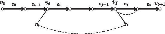
In practice, the most commonly employed safe strings are those spelled by maximal unitigs, where unitigs are paths whose internal nodes have in- and out-degree 1. Figure 2 shows an example of the output of the unitig algorithm, and also illustrates that it does not identify all safe strings. The EULER assembler (Pevzner et al., 2001) takes unitigs a step further and identifies strings spelled by paths whose internal nodes have out-degree equal to 1 (with no constraint on their in-degree). It can be shown that such strings are also safe. However, the most complete characterization of safe strings that we found is given by the Y-to-V algorithm (Medvedev et al., 2007; Jackson, 2009; Kingsford et al., 2010). Consider a node v with exactly one in-neighbor u and more than one out-neighbors w₁,…,w_d. The Y-to-V reduction applied to v removes v and its incident edges from the graph and adds nodes v₁,…,v_d with edges from u to v_i and from v_i to w_i, for all 1 ≤ i ≤ d. The Y-to-V reduction is defined symmetrically for nodes with out-degree exactly 1 and in-degree greater than 1. Figure 1 illustrates the definition. The Y-to-V algorithm proceeds by repeatedly applying Y-to-V reductions, in arbitrary order, for as long as possible. The algorithm then outputs the strings spelled by the maximal unitigs in the final graph (see Fig. 2d for an example). The Y-to-V algorithm can also be shown to be safe, but, as we will show in Figure 2, it does not always output all the safe strings. We are not aware of any study that compares the merits of Y-to-V contigs with those of unitigs, and we therefore perform this analysis in Section 8.

FIG. 1.

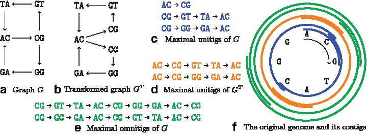
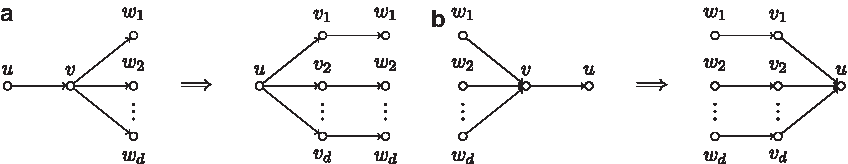
The output of the three algorithms on the edge-centric de Bruijn graph G from (a), built from the circular string in (f). Each contig is drawn as an arc on the wheel in (f). (c) The maximal unitigs of G; (b) the Y-to-V reduction is applied to node CG and the resulting graph G^T is shown; no more reductions are applicable and G^T has two maximal unitigs, shown in (d); (e) the maximal omnitigs of G; in this particular example, they are also circular edge-covering walks of G, and one can be obtained from the other by a circular permutation. Note that this example illustrates that the Y-to-V algorithm does not always output all safe strings, because its output (d) does not contain the strings of (e).

FIG. 2.

The Y-to-V reduction applied to node v. (a) v has in-degree exactly 1; (b) v has out-degree exactly 1.

3. Basic Definitions

Given a string x and an index 1 ≤ i ≤ |x|, we define pre(x, i) and suf(x, i) as its length i prefix and suffix, respectively. If x and y are two strings, and suf(x, k) = pre(y, k) for some k ≤ |x| − 1, then we define x ⨁^k y as x[1..|x|−k] concatenated with y. This captures the notion of merging two overlapping strings. A k-mer of x is a substring of length k. Let R be a set of strings, which we equivalently refer to as reads. The node-centric de Bruijn graph built on R, denoted \documentclass{aastex}\usepackage{amsbsy}\usepackage{amsfonts}\usepackage{amssymb}\usepackage{bm}\usepackage{mathrsfs}\usepackage{pifont}\usepackage{stmaryrd}\usepackage{textcomp}\usepackage{portland, xspace}\usepackage{amsmath, amsxtra}\pagestyle{empty}\DeclareMathSizes{10}{9}{7}{6}\begin{document} $${ \rm{DB}}_{nc}^k ( R )$$ \end{document} , is the graph whose set of nodes is the set of all k-mers of R, in which there is an edge from a node x to a node y iff suf(x, k − 1) = pre(y, k − 1) (Chikhi and Rizk, 2012). The edge-centric de Bruijn graph built on R, denoted \documentclass{aastex}\usepackage{amsbsy}\usepackage{amsfonts}\usepackage{amssymb}\usepackage{bm}\usepackage{mathrsfs}\usepackage{pifont}\usepackage{stmaryrd}\usepackage{textcomp}\usepackage{portland, xspace}\usepackage{amsmath, amsxtra}\pagestyle{empty}\DeclareMathSizes{10}{9}{7}{6}\begin{document} $${ \rm{DB}}_{{ \rm{ec}}}^k ( R )$$ \end{document} is defined similarly to \documentclass{aastex}\usepackage{amsbsy}\usepackage{amsfonts}\usepackage{amssymb}\usepackage{bm}\usepackage{mathrsfs}\usepackage{pifont}\usepackage{stmaryrd}\usepackage{textcomp}\usepackage{portland, xspace}\usepackage{amsmath, amsxtra}\pagestyle{empty}\DeclareMathSizes{10}{9}{7}{6}\begin{document} $${ \rm{DB}}_{nc}^k ( R )$$ \end{document} , with the difference that there is an edge from x to y iff suf(x, k − 1) = pre(y, k − 1) and x ⨁^k−1 y is a substring of some string in R (Idury and Waterman, 1995). The weight of the edges of \documentclass{aastex}\usepackage{amsbsy}\usepackage{amsfonts}\usepackage{amssymb}\usepackage{bm}\usepackage{mathrsfs}\usepackage{pifont}\usepackage{stmaryrd}\usepackage{textcomp}\usepackage{portland, xspace}\usepackage{amsmath, amsxtra}\pagestyle{empty}\DeclareMathSizes{10}{9}{7}{6}\begin{document} $${ \rm{DB}}_{nc}^k ( R )$$ \end{document} and \documentclass{aastex}\usepackage{amsbsy}\usepackage{amsfonts}\usepackage{amssymb}\usepackage{bm}\usepackage{mathrsfs}\usepackage{pifont}\usepackage{stmaryrd}\usepackage{textcomp}\usepackage{portland, xspace}\usepackage{amsmath, amsxtra}\pagestyle{empty}\DeclareMathSizes{10}{9}{7}{6}\begin{document} $${ \rm{DB}}_{ec}^k ( R )$$ \end{document} is k − 1.

Let G be a graph, possibly with parallel edges and self-loops. The number of nodes and edges in a graph is denoted by n and m, respectively. We use N⁻(v) to denote the set of in-neighbors and N⁺(v) to denote the set of out-neighbors of a node v. A walk w is a sequence (v₀, e₀, v₁, e₁,…,v_t, e_t, v_t₊₁) where v₀,…,v_t₊₁ are nodes, and each e_i is an edge from v_i to v_i₊₁, and t ≥ − 1. Its length is its number of edges, namely t + 1. A path is a walk in which the nodes are all distinct, except possibly the first and last nodes may be the same, in which case it will also be called a cycle. Walks and paths of length at least 1 are called proper. A walk whose first and last nodes coincide is called circular walk. A path (walk) with first node u and last node v will be called a path (walk) from u to v, and denoted as (u)-(v) path (walk). A walk is called node-covering if it passes through each node of G, and edge-covering if it passes through each edge of G. The notions of prefix and subwalk are defined for walks in the natural way, for example, by interpreting a walk to be a string made up by concatenating its edges. In particular, we say that a walk w₁ is a subwalk of a circular walk w₂ if w₁ interpreted as string is a substring of w₂ interpreted as circular string. In this article, we allow strings and walks to have overlapping extremities when viewed as substrings of a circular string, that is, when aligned to a circular string (see, e.g., the two omnitigs from Figure 2f that have an overlapping tail and head).

Let ℓ be a function labeling the nodes of G and let c be a function giving weights to the edges (intuitively, c should represent the length of overlaps). One can apply the notion of string spelled by a walk w = (v₀, e₀, v₁, e₁,…,v_t, e_t, v_t₊₁) by defining the string spelled by w as spell \documentclass{aastex}\usepackage{amsbsy}\usepackage{amsfonts}\usepackage{amssymb}\usepackage{bm}\usepackage{mathrsfs}\usepackage{pifont}\usepackage{stmaryrd}\usepackage{textcomp}\usepackage{portland, xspace}\usepackage{amsmath, amsxtra}\pagestyle{empty}\DeclareMathSizes{10}{9}{7}{6}\begin{document} $$( w ) = \ell ( {v_0} ) { \oplus ^{c ( {e_0} ) }} \ell ( {v_1} ){ \oplus ^{c ( {e_1} ) }} \cdots { \oplus ^{c ( {e_t} ) }} \ell ( {v_{t + 1}} )$$ \end{document} . When the walk w is circular (thus v_t₊₁ = v₀), then spell(w) will be interpreted as the circular string obtained by overlapping the strings ℓ(v₀) and ℓ(v_t₊₁).

4. Problem Formulation

There are various theoretical approaches to formulating the assembly problem. Here, we adopt a model that captures the most popular models: the node-centric de Bruijn graph, the edge-centric de Bruijn graph, and the string graph (Myers, 2005). We generalize these using the notion of a genome graph:

Definition 1 (Genome graph). A graph G with edge-weights given by c and node-labels is a genome graph if and only if (1) for every edge e = (u, v), suf (u, c(e)) = pre(v, c(e)) and (2) for any two walks w₁ and w₂, w₁ is a subwalk of w₂ if and only if spell(w₁) is a substring of spell(w₂).

Both node- and edge-centric de Bruijn graphs are genome graphs, directly by their definition. Similarly, the interested reader can verify that string graphs, as commonly defined by Myers (2005), Nagarajan and Pop (2009), Medvedev et al. (2007), Simpson and Durbin (2010), are genome graphs. Intuitively, the first condition states that the edge-weights represent the length of overlaps between strings, whereas the second condition prohibits a certain redundancy in the graph. It can be broken if, for example, there are nodes with duplicate labels, or if some labels are substrings of others. Or, for string graphs, it can be broken if transitive edges are not removed from the graph (Myers, 2005). We now augment a genome graph with a rule defining a “genomic reconstruction.”

Definition 2 (Graph model). A graph model \documentclass{aastex}\usepackage{amsbsy}\usepackage{amsfonts}\usepackage{amssymb}\usepackage{bm}\usepackage{mathrsfs}\usepackage{pifont}\usepackage{stmaryrd}\usepackage{textcomp}\usepackage{portland, xspace}\usepackage{amsmath, amsxtra}\pagestyle{empty}\DeclareMathSizes{10}{9}{7}{6}\begin{document} $${\cal G}$$ \end{document} is defined by

• An algorithm that transforms a set of reads R into a genome graph, denoted by \documentclass{aastex}\usepackage{amsbsy}\usepackage{amsfonts}\usepackage{amssymb}\usepackage{bm}\usepackage{mathrsfs}\usepackage{pifont}\usepackage{stmaryrd}\usepackage{textcomp}\usepackage{portland, xspace}\usepackage{amsmath, amsxtra}\pagestyle{empty}\DeclareMathSizes{10}{9}{7}{6}\begin{document} $${\cal G}$$ \end{document} (R).

• A rule that determines whether a walk in \documentclass{aastex}\usepackage{amsbsy}\usepackage{amsfonts}\usepackage{amssymb}\usepackage{bm}\usepackage{mathrsfs}\usepackage{pifont}\usepackage{stmaryrd}\usepackage{textcomp}\usepackage{portland, xspace}\usepackage{amsmath, amsxtra}\pagestyle{empty}\DeclareMathSizes{10}{9}{7}{6}\begin{document} $${\cal G}$$ \end{document} (R) is a genomic reconstruction.

Intuitively, a genomic reconstruction spells a genome that could have generated the observed set of reads R. In this article, we consider two graph models. In the edge-centric model, a genomic reconstruction is a circular edge-covering walk; its underlying genome graph can be, for example, an edge-centric de Bruijn graph. In the node-centric model, a genomic reconstruction is a circular node-covering walk; its underlying genome graph can be a node-centric de Bruijn graph or a string graph. As mentioned in the introduction, we assume, without always explicitly stating it onward, that \documentclass{aastex}\usepackage{amsbsy}\usepackage{amsfonts}\usepackage{amssymb}\usepackage{bm}\usepackage{mathrsfs}\usepackage{pifont}\usepackage{stmaryrd}\usepackage{textcomp}\usepackage{portland, xspace}\usepackage{amsmath, amsxtra}\pagestyle{empty}\DeclareMathSizes{10}{9}{7}{6}\begin{document} $${\cal G}$$ \end{document} (R) contains at least one genomic reconstruction, and for technical reasons—see the proof of Lemma 1—that \documentclass{aastex}\usepackage{amsbsy}\usepackage{amsfonts}\usepackage{amssymb}\usepackage{bm}\usepackage{mathrsfs}\usepackage{pifont}\usepackage{stmaryrd}\usepackage{textcomp}\usepackage{portland, xspace}\usepackage{amsmath, amsxtra}\pagestyle{empty}\DeclareMathSizes{10}{9}{7}{6}\begin{document} $${\cal G}$$ \end{document} (R) is always different from a single cycle. In fact, in the latter case, the assembly problem is trivial.

We now define the strings that belong to all genomic reconstructions.

Definition 3 (Safe string). Given a set of reads R and a graph model \documentclass{aastex}\usepackage{amsbsy}\usepackage{amsfonts}\usepackage{amssymb}\usepackage{bm}\usepackage{mathrsfs}\usepackage{pifont}\usepackage{stmaryrd}\usepackage{textcomp}\usepackage{portland, xspace}\usepackage{amsmath, amsxtra}\pagestyle{empty}\DeclareMathSizes{10}{9}{7}{6}\begin{document} $${\cal G}$$ \end{document} , a string s is said to be a safe string for \documentclass{aastex}\usepackage{amsbsy}\usepackage{amsfonts}\usepackage{amssymb}\usepackage{bm}\usepackage{mathrsfs}\usepackage{pifont}\usepackage{stmaryrd}\usepackage{textcomp}\usepackage{portland, xspace}\usepackage{amsmath, amsxtra}\pagestyle{empty}\DeclareMathSizes{10}{9}{7}{6}\begin{document} $${\cal G}$$ \end{document} (R) if for every genomic reconstruction w of \documentclass{aastex}\usepackage{amsbsy}\usepackage{amsfonts}\usepackage{amssymb}\usepackage{bm}\usepackage{mathrsfs}\usepackage{pifont}\usepackage{stmaryrd}\usepackage{textcomp}\usepackage{portland, xspace}\usepackage{amsmath, amsxtra}\pagestyle{empty}\DeclareMathSizes{10}{9}{7}{6}\begin{document} $${\cal G}$$ \end{document} (R), s is a substring of spell(w).

In particular, for a node-centric (respectively, edge-centric) graph model \documentclass{aastex}\usepackage{amsbsy}\usepackage{amsfonts}\usepackage{amssymb}\usepackage{bm}\usepackage{mathrsfs}\usepackage{pifont}\usepackage{stmaryrd}\usepackage{textcomp}\usepackage{portland, xspace}\usepackage{amsmath, amsxtra}\pagestyle{empty}\DeclareMathSizes{10}{9}{7}{6}\begin{document} $${\cal G}$$ \end{document} , a string s is safe if for every circular node-covering (respectively, edge-covering) walk w, s is a substring of spell(w). It also follows from the definitions (again assuming no gaps in coverage and no errors in the reads) that if the genome graph is \documentclass{aastex}\usepackage{amsbsy}\usepackage{amsfonts}\usepackage{amssymb}\usepackage{bm}\usepackage{mathrsfs}\usepackage{pifont}\usepackage{stmaryrd}\usepackage{textcomp}\usepackage{portland, xspace}\usepackage{amsmath, amsxtra}\pagestyle{empty}\DeclareMathSizes{10}{9}{7}{6}\begin{document} $${ \rm{DB}}_{nc}^k ( R )$$ \end{document} or \documentclass{aastex}\usepackage{amsbsy}\usepackage{amsfonts}\usepackage{amssymb}\usepackage{bm}\usepackage{mathrsfs}\usepackage{pifont}\usepackage{stmaryrd}\usepackage{textcomp}\usepackage{portland, xspace}\usepackage{amsmath, amsxtra}\pagestyle{empty}\DeclareMathSizes{10}{9}{7}{6}\begin{document} $${ \rm{DB}}_{ec}^k ( R )$$ \end{document} , then a string is safe if it is a substring of every circular string with the same set of k-mers, or (k + 1)-mers respectively, as R.

Solving the following problem gives all the information that can be safely retrieved from a graph model.

Definition 4 (The safe and complete contig assembly problem). Given a set of reads R and a graph model \documentclass{aastex}\usepackage{amsbsy}\usepackage{amsfonts}\usepackage{amssymb}\usepackage{bm}\usepackage{mathrsfs}\usepackage{pifont}\usepackage{stmaryrd}\usepackage{textcomp}\usepackage{portland, xspace}\usepackage{amsmath, amsxtra}\pagestyle{empty}\DeclareMathSizes{10}{9}{7}{6}\begin{document} $${\cal G}$$ \end{document} , output all the safe strings for \documentclass{aastex}\usepackage{amsbsy}\usepackage{amsfonts}\usepackage{amssymb}\usepackage{bm}\usepackage{mathrsfs}\usepackage{pifont}\usepackage{stmaryrd}\usepackage{textcomp}\usepackage{portland, xspace}\usepackage{amsmath, amsxtra}\pagestyle{empty}\DeclareMathSizes{10}{9}{7}{6}\begin{document} $${\cal G}$$ \end{document} (R).

In this article, we solve this problem for the node- and edge-centric models already defined. In Sections 5 and 6, we first deal with the edge-centric model, and then in Section 7, we show how these results can be modified for the node-centric model.

As a technical aside, our algorithms will output only maximal safe strings, in the sense that they are not a substring of any other safe string. In fact, this is desirable in practice, and moreover, the set of all safe strings is the set of all substrings of the maximal safe strings.

A note on assumptions: Our model makes three implicit assumptions, as outlined at the end of the Introduction. Here, we observe that such assumptions are necessary to prove even the simplest desired property: that the unitig algorithm outputs only safe strings. Let w = (v₀,e₀,v₁,e₁,v₂) be a unitig in an edge-centric de Bruijn graph G built from the (k + 1)-mers of a genome S. If the genome is not circular [assumption (i)], then, for example, the last k-mer of S can be v₀, its first k-mer can be v₁, the string v₀ ⨁^k v₁ can appear inside S, but v₀ ⨁^k v₁ ⨁^k v₂ does not have to appear in S. If there are gaps in coverage [assumption (ii)], then both an in-neighbor v′ and an out-neighbor v′′ of v₁ may be missing from G making w look safe, whereas in reality v₀ ⨁^k v₁ ⨁^k v₂ may not be a substring of S. If a read contains a sequencing error [assumption (iii)], then this creates a bubble in G with one of its paths being a unitig not spelling a substring of S.

5. Characterization of Safe Strings: Omnitigs

In this section, we provide a characterization of walks that spell safe strings (see Fig. 3 for an illustration). This characterization is the basis of our omnitig algorithm in the next section.

FIG. 3.

An illustration of the omnitig definition, edge-centric model.

Definition 5 (Omnitig, edge-centric model). Let G be a directed graph and let w = (v₀, e₀, v₁, e₁, …, v_t, e_t, v_t₊₁) be a walk in G. We say that w is a omnitig if and only if for all 1 ≤ i ≤ j ≤ t, there is no proper (v_j)-(v_i) path with first edge different from e_j, and last edge different from e_i₋₁.

The following theorem proves that the omnitigs spell all the safe strings, using the help of an intermediary characterization of omnitigs.

Theorem 1. Given an edge-centric graph model G = \documentclass{aastex}\usepackage{amsbsy}\usepackage{amsfonts}\usepackage{amssymb}\usepackage{bm}\usepackage{mathrsfs}\usepackage{pifont}\usepackage{stmaryrd}\usepackage{textcomp}\usepackage{portland, xspace}\usepackage{amsmath, amsxtra}\pagestyle{empty}\DeclareMathSizes{10}{9}{7}{6}\begin{document} $${\cal G}$$ \end{document} (R) built for a set of reads R, and a string s, the following three statements are equivalent:

(1) s is a safe string for G;

(2) s is spelled by a walk w = (v₀, e₀, v₁, e₁, …, v_t, e_t, v_t₊₁) in G and w is an omnitig;

(3) s is spelled by a walk w = (v₀, e₀, v₁, e₁, …, v_t, e_t, v_t₊₁) in G and for all 1 ≤ j ≤ t all proper v_j−v_j (circular) walks w′ fulfill at least one of the following conditions:

(i) the subwalk (v_j, e_j, …, v_t, e_t, v_t₊₁) of w is a prefix w′, or

(ii) the subwalk (v₀, e₀, …, v_j_-1, e_j₋₁, v_j) of w is a suffix of w′, or

(iii) w is a subwalk of w′.

We prove Theorem 1 by proving the cyclical sequence of implications (1) ⇒ (2) ⇒ (3) ⇒ (1).

Proof of (1) ⇒ (2). Assume that s is a safe string for G. By definition of a genome graph, s is spelled by a unique walk in G. Let w = (v₀, e₀, v₁, e₁, …, v_t, e_t, v_t₊₁) be this walk, and let A be a circular edge-covering walk of G; thus A contains w as subwalk, and s is a substring of spell(A).

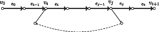
Assume for a contradiction that there exist 1 ≤ i ≤ j ≤ t, and a proper v_j−v_i path p with first edge different from e_j and last edge different from e_i₋₁. From A, we construct another circular edge-covering walk B of G that does not contain w as subwalk, and hence, by the definition of a genome graph, also spell(B) does not contain s as substring. This contradicts the safeness of s. Whenever A visits node v_j, then B follows the v_j−v_i path p, then follows (v_i, e_i, …, e_j₋₁, v_j), and finally continues as A. To see that w does not appear as a subwalk of B, consider the subwalk w′ = (v_i₋₁,e_i₋₁,v_i,e_i,…,e_j₋₁,v_j,e_j,v_j₊₁) of w (recall that 1 ≤ i ≤ j ≤ t). Since p is proper, and its first edge is different from e_j and its last edge is different from e_i₋₁, then, by construction, the only way that w′ can appear in B is as a subwalk of p. However, this implies that both v_j and v_i appear twice on p, contradicting the fact that p is a path. ■

Proof of (2) ⇒ (3). Suppose that w is an omnitig, and assume for a contradiction that there exists a proper v_j−v_j walk (for some 1 ≤ j ≤ t) not satisfying (i)–(iii). Let w′ be the shortest such walk. Since w′ does not have (v_j,e_j,…,v_t,e_t,v_t₊₁) as prefix, then there exists a first node v_ℓ on w, j ≤ ℓ ≤ t, such that from v_ℓ, w′ continues with an edge \documentclass{aastex}\usepackage{amsbsy}\usepackage{amsfonts}\usepackage{amssymb}\usepackage{bm}\usepackage{mathrsfs}\usepackage{pifont}\usepackage{stmaryrd}\usepackage{textcomp}\usepackage{portland, xspace}\usepackage{amsmath, amsxtra}\pagestyle{empty}\DeclareMathSizes{10}{9}{7}{6}\begin{document} $${e^{\prime} _ \ell } \, \ne {e_ \ell }$$ \end{document} . Symmetrically, since w′ does not have (v₀, e₀,…,v_j₋₁, e_j₋₁, v_j) as suffix, let v_i be the last node of w, 1 ≤ i ≤ j, such that before entering v_i, the walk w′ uses an edge \documentclass{aastex}\usepackage{amsbsy}\usepackage{amsfonts}\usepackage{amssymb}\usepackage{bm}\usepackage{mathrsfs}\usepackage{pifont}\usepackage{stmaryrd}\usepackage{textcomp}\usepackage{portland, xspace}\usepackage{amsmath, amsxtra}\pagestyle{empty}\DeclareMathSizes{10}{9}{7}{6}\begin{document} $${e^{\prime} _{i - 1}} \ne {e_{i - 1}}$$ \end{document} . Let \documentclass{aastex}\usepackage{amsbsy}\usepackage{amsfonts}\usepackage{amssymb}\usepackage{bm}\usepackage{mathrsfs}\usepackage{pifont}\usepackage{stmaryrd}\usepackage{textcomp}\usepackage{portland, xspace}\usepackage{amsmath, amsxtra}\pagestyle{empty}\DeclareMathSizes{10}{9}{7}{6}\begin{document} $${w^{\prime} _0}$$ \end{document} denote the subwalk of w′ between \documentclass{aastex}\usepackage{amsbsy}\usepackage{amsfonts}\usepackage{amssymb}\usepackage{bm}\usepackage{mathrsfs}\usepackage{pifont}\usepackage{stmaryrd}\usepackage{textcomp}\usepackage{portland, xspace}\usepackage{amsmath, amsxtra}\pagestyle{empty}\DeclareMathSizes{10}{9}{7}{6}\begin{document} $${e^{\prime} _ \ell }$$ \end{document} and \documentclass{aastex}\usepackage{amsbsy}\usepackage{amsfonts}\usepackage{amssymb}\usepackage{bm}\usepackage{mathrsfs}\usepackage{pifont}\usepackage{stmaryrd}\usepackage{textcomp}\usepackage{portland, xspace}\usepackage{amsmath, amsxtra}\pagestyle{empty}\DeclareMathSizes{10}{9}{7}{6}\begin{document} $${e^{\prime} _{i - 1}}$$ \end{document} (inclusive). If \documentclass{aastex}\usepackage{amsbsy}\usepackage{amsfonts}\usepackage{amssymb}\usepackage{bm}\usepackage{mathrsfs}\usepackage{pifont}\usepackage{stmaryrd}\usepackage{textcomp}\usepackage{portland, xspace}\usepackage{amsmath, amsxtra}\pagestyle{empty}\DeclareMathSizes{10}{9}{7}{6}\begin{document} $${w^{\prime} _0}$$ \end{document} is a path, then w″ is a proper v_ℓ−v_i path, 1 ≤ i ≤ ℓ ≤ t, whose first edge \documentclass{aastex}\usepackage{amsbsy}\usepackage{amsfonts}\usepackage{amssymb}\usepackage{bm}\usepackage{mathrsfs}\usepackage{pifont}\usepackage{stmaryrd}\usepackage{textcomp}\usepackage{portland, xspace}\usepackage{amsmath, amsxtra}\pagestyle{empty}\DeclareMathSizes{10}{9}{7}{6}\begin{document} $${e^{\prime} _ \ell }$$ \end{document} is different from e_ℓ, and its last edge \documentclass{aastex}\usepackage{amsbsy}\usepackage{amsfonts}\usepackage{amssymb}\usepackage{bm}\usepackage{mathrsfs}\usepackage{pifont}\usepackage{stmaryrd}\usepackage{textcomp}\usepackage{portland, xspace}\usepackage{amsmath, amsxtra}\pagestyle{empty}\DeclareMathSizes{10}{9}{7}{6}\begin{document} $${e^{\prime} _{i - 1}}$$ \end{document} is different from e_i₋₁, which contradicts the fact that w is an omnitig. We now prove that w′ is in fact a path.

Suppose for a contradiction that it is not, thus that it contains a cycle c, with c ≠ w′. Let w′′ be the walk obtained from w′ by removing the cycle c. Observe that w″ is still a proper v_j−v_j walk. We show that w″ still does not satisfy (i)–(iii), which will contradict the minimality of w′. Assume for a contradiction that w″ satisfies at least one of (i), (ii), or (iii).

First, if w″ satisfies (i), this implies that the edge \documentclass{aastex}\usepackage{amsbsy}\usepackage{amsfonts}\usepackage{amssymb}\usepackage{bm}\usepackage{mathrsfs}\usepackage{pifont}\usepackage{stmaryrd}\usepackage{textcomp}\usepackage{portland, xspace}\usepackage{amsmath, amsxtra}\pagestyle{empty}\DeclareMathSizes{10}{9}{7}{6}\begin{document} $${e^{\prime} _ \ell }$$ \end{document} out going from v_ℓ belongs to c, and after traversing c, the walk w′ continues through (v_ℓ, e_ℓ,…,v_t, e_t, v_t₊₁; Fig. 4a, b). Let v_p be the node of w with greatest index p ∈{0,…,ℓ} that c visits with an edge e′ = (v, v_p) not on w. Such a node exists because c is a cycle and it must return to v_ℓ. If p ≥ 1 (Fig. 4a), then c does not satisfy (i)–(iii). Since c is proper and passes through v_ℓ, where 1 ≤ ℓ ≤ t, this contradicts the minimality of w′. Therefore, p = 0 (Fig. 4b), and thus, the initial v_j−v_j walk w′ (containing c as subwalk) visits (v₀,e₀,…,v_ℓ), and then continues through (v_ℓ,e_ℓ,…,v_t,e_t,v_t₊₁). This implies that w′ contains w as subwalk, which contradicts the choice of w′.

FIG. 4.

Illustration of three cases in the proof of the implication (2) ⇒ (3) of Theorem 1.

The second case when w″ satisfies (ii) is entirely symmetric.

Third, assume that w″ contains w as subwalk. Since w is not a subwalk of w′, this implies that c is a proper v_r−v_r walk, for some 1 ≤ r ≤ t, not satisfying (i)–(iii), which again contradicts the minimality of w′ (Fig. 4c). This completes the proof of (2) ⇒ (3) ■

Proof of (3) ⇒ (1). Assume w satisfies (3), and let A be a circular edge-covering walk of G. We need to show that w is a subwalk of A. Let w_j = (v₀,e₀,…,v_j₋₁,e_j₋₁,v_j) be the longest prefix of w that A ever traverses, ending at some v_j. Since A covers all edges, then it also covers e₀, and thus j ≥ 1. Suppose for a contradiction that j ≠ t + 1.

Since A is circular and covers all edges of G, then after traversing w_j, the walk A eventually visits the edge e_j. The walk A may visit v_j multiple times before traversing the edge e_j. Let w′ denote the subwalk of A between the last two occurrences of v_j before A traverses the edge e_j. Since w′ is a proper v_j−v_j walk, 1 ≤ j ≤ t, and w satisfies (3), we have that one of the following must hold:

• the walk (v_j,e_j,…,v_t,e_t,v_t₊₁) is a prefix of w′: this contradicts the fact that w′ is a subwalk of A between v_j and the immediately next occurrence of e_j (since in this case w′ contains e_j);

• the walk (v₀,e₀,…,v_j₋₁,e_j₋₁,v_j) is a suffix of w′: this implies that (w′, e_j, v_j₊₁) is a longer prefix of w that is a subwalk of A, contradicting the maximality of w_j;

• the walk w appears on w′: since w′ is a subwalk of A, this implies that also w is a subwalk of A, contradicting again the maximality of w_j.

6. Omnitig Algorithm

In this section, we use Theorem 1 to give the omnitig algorithm (Algorithm 1) and prove that it runs in polynomial time (Theorem 2). The algorithm finds all maximal omnitigs of \documentclass{aastex}\usepackage{amsbsy}\usepackage{amsfonts}\usepackage{amssymb}\usepackage{bm}\usepackage{mathrsfs}\usepackage{pifont}\usepackage{stmaryrd}\usepackage{textcomp}\usepackage{portland, xspace}\usepackage{amsmath, amsxtra}\pagestyle{empty}\DeclareMathSizes{10}{9}{7}{6}\begin{document} $${\cal G}$$ \end{document} (R), which, by Theorem 1, are exactly the maximal safe strings of \documentclass{aastex}\usepackage{amsbsy}\usepackage{amsfonts}\usepackage{amssymb}\usepackage{bm}\usepackage{mathrsfs}\usepackage{pifont}\usepackage{stmaryrd}\usepackage{textcomp}\usepackage{portland, xspace}\usepackage{amsmath, amsxtra}\pagestyle{empty}\DeclareMathSizes{10}{9}{7}{6}\begin{document} $${\cal G}$$ \end{document} (R). Our algorithm is based on the following observation, which follows directly from the definition of omnitigs:

Observation 1. Consider a walk w′ = (v₀, e₀,…,e_t−₁,v_t,e_t,v_t₊₁) of length at least 2, and consider its subwalk w = (v₀,e₀,…,e_t−₁,v_t). Then w′ is an omnitig if and only if (i) w is an omnitig and (ii) for all 0 ≤ i ≤ t − 1, there is no proper v_t−v_i path with first edge different from e_t and last edge different from e_i−₁.

Algorithm 1:

Omnitig algorithm to find all safe strings of a graph G.

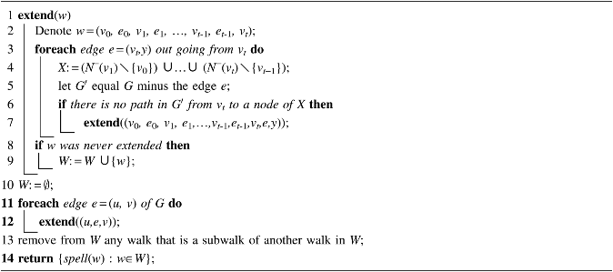
The idea of the algorithm is to start an exhaustive traversal of G from every edge (Lines 11 and 12), which by definition is an omnitig, and to keep traversing edges as long as the current walk is an omnitig. An omnitig w is thus recursively constructed, by possibly extending to the right with each edge e out going from its last vertex (Lines 3–7). If w extended with e is not an omnitig, then we abandon this extension because Observation 1 tells us that no further extension could be an omnitig. To check whether this extension is an omnitig or not, it is enough to check whether condition (ii) of Observation 1 is satisfied. Condition (i) is automatically satisfied because of the structure of the algorithm—we extend only walks that are omnitigs. The omnitigs found are saved in a set W (Line 9), except for those omnitigs that are obviously nonmaximal (Line 8). In the final step (Lines 13 and 14), we remove the nonmaximal omnitigs from W and report the rest.

To check whether condition (ii) is satisfied (Lines 4–6), we take the set X (Line 4) and check whether there is a path starting with an edge out going from v_t and different from e, and leading to a node of X. The correctness of this procedure can be seen as follows. If there is no such path, then we know that there is no path satisfying (ii). If we do find a path p from v_t to some in-neighbor x ∈X of some v_i, and p does not use v_i, then the path obtained by extending p to v_i contradicts (ii). If p contains v_i, then such an extension is not possible, because a path cannot repeat a vertex; however, we will show that p cannot use v_i by contradiction. Assume that it does, and observe that after passing through v_i, the path p cannot pass again through v_t. Let v_j, i ≤ j < t, be the first vertex that p visits after v_i such that from v_j it continues with an edge e′ ≠ e_j. Let p′ denote the v_j−x subpath of p from v_j until x. We obtained that p′ followed by v_i is a proper v_j−v_i path with first edge different from e_j, last edge different from e_i−₁, and 1 ≤ i ≤ j ≤ t. This contradicts the fact that w (the walk we are extending) is an omnitig.

Next, we show that the algorithm runs in polynomial time. First, we show that the number of omnitigs included in W and their length, before removal of nonmaximal omnitigs, is polynomial:

Lemma 1. Let W be a set of omnitigs in an edge-centric graph model \documentclass{aastex}\usepackage{amsbsy}\usepackage{amsfonts}\usepackage{amssymb}\usepackage{bm}\usepackage{mathrsfs}\usepackage{pifont}\usepackage{stmaryrd}\usepackage{textcomp}\usepackage{portland, xspace}\usepackage{amsmath, amsxtra}\pagestyle{empty}\DeclareMathSizes{10}{9}{7}{6}\begin{document} $${\cal G}$$ \end{document} (R), whose genome graph is different from a single cycle. Furthermore, suppose no omnitig in W is a prefix of another omnitig in W. Then, |W| ≤ nm and the length of any omnitig in W is O(nm).

Proof. We first show that we can visit the edges of G = \documentclass{aastex}\usepackage{amsbsy}\usepackage{amsfonts}\usepackage{amssymb}\usepackage{bm}\usepackage{mathrsfs}\usepackage{pifont}\usepackage{stmaryrd}\usepackage{textcomp}\usepackage{portland, xspace}\usepackage{amsmath, amsxtra}\pagestyle{empty}\DeclareMathSizes{10}{9}{7}{6}\begin{document} $${\cal G}$$ \end{document} (R) with a circular edge-covering walk C of at most nm nodes. Let e₀,…,e_m₋₁ be an arbitrary order of the edges of G. Since we assume that G admits one genomic reconstruction, then G is strongly connected. Thus, from every end extremity of e_i, there is a path to the start extremity of e_{(i+1) mod m}, 0 ≤ i ≤ m − 1, of length at most n − 1. Therefore, C can be constructed to first visit e₀, then to follow such a path until e₁, and so on until e_m₋₁, from where it follows such a path back to e₀.

By Theorem 1, we have that any omnitig of G is a subwalk of C. We can associate every w ∈W with all the start positions in C (in terms of nodes) where it is a subwalk. Because W does not contain walks that are prefixes of other walks, a position of C can have at most one walk associated with it. Since |C| ≤ nm, W can contain at most nm walks.

It remains to prove that the length of any omnitig in W is O(nm). To simplify notation, rename C as (v₀, e₀, v₁, e₁,…,v_t, e_t, v_t₊₁) with v_t₊₁ = v₀. Since G is different from a single cycle, then there exist v_j and v_i on C, such that e = (v_j, v_i) is an edge of G, and \documentclass{aastex}\usepackage{amsbsy}\usepackage{amsfonts}\usepackage{amssymb}\usepackage{bm}\usepackage{mathrsfs}\usepackage{pifont}\usepackage{stmaryrd}\usepackage{textcomp}\usepackage{portland, xspace}\usepackage{amsmath, amsxtra}\pagestyle{empty}\DeclareMathSizes{10}{9}{7}{6}\begin{document} $$e\, \notin \, \left\{ {{e_j}, \,{e_{i - 1}}} \right\} $$ \end{document} . Any omnitig (thus a subwalk of C) cannot contain twice v_j and v_i as internal nodes, since otherwise the proper path (v_j, e, v_i) violates the omnitig definition. Thus the length of any omnitig is O(nm). ■

(As an aside, it remains open whether the bound on |W| can be reduced to m, which is the case for unitigs; our experiments in Section 8 suggest that this may be the case in practice.) Note that Line 8 guarantees that W, before removal of subwalks in Line 13, satisfies the prefix condition of Lemma 1. Lemma 1 then implies that reporting one omnitig by our algorithm takes polynomial time, and there are only polynomially many omnitigs reported. Furthermore, removing the nonmaximal omnitigs (Line 13) can be done in linear time in the sum of the omnitig lengths, by appropriately traversing a suffix tree constructed from them. Thus, we have our main theorem:

Theorem 2. Let R be a set of reads and let \documentclass{aastex}\usepackage{amsbsy}\usepackage{amsfonts}\usepackage{amssymb}\usepackage{bm}\usepackage{mathrsfs}\usepackage{pifont}\usepackage{stmaryrd}\usepackage{textcomp}\usepackage{portland, xspace}\usepackage{amsmath, amsxtra}\pagestyle{empty}\DeclareMathSizes{10}{9}{7}{6}\begin{document} $${\cal G}$$ \end{document} (R) be an edge-centric graph model. Algorithm 1 outputs in polynomial time all safe strings of \documentclass{aastex}\usepackage{amsbsy}\usepackage{amsfonts}\usepackage{amssymb}\usepackage{bm}\usepackage{mathrsfs}\usepackage{pifont}\usepackage{stmaryrd}\usepackage{textcomp}\usepackage{portland, xspace}\usepackage{amsmath, amsxtra}\pagestyle{empty}\DeclareMathSizes{10}{9}{7}{6}\begin{document} $${\cal G}$$ \end{document} (R).

Finally, we note some implementation details that are crucial in practice. Before starting, we apply the Y-to-V algorithm and the standard graph compaction algorithm to compact unitigs (Chikhi et al., 2014). This significantly reduces the number of nodes/edges in the graph without changing the maximal safe strings. We also precompute all omnitigs of length 2 and store them in a hash table so that whenever we want to extend the omnitig w in Line 6, we check beforehand whether the pair (e_t₋₁,e) is stored in the hash table. This significantly limits, in practice, the number of graph traversals we have to do at Line 6. Finally, we do not compute the set X every time, but instead incrementally built it up as we extend the omnitig w. Our implementation is freely available for use (https://github.com/alexandrutomescu/complete-contigs).

7. Node-Centric Model

In this section, we obtain analogous results for node-centric models, although both the definitions, algorithms, and proofs need to be modified. The following definition is similar to that for the edge-centric model, the only addition being its second bullet (see Fig. 5 for an illustration).

FIG. 5.

An illustration of the omnitig definition, node-centric model.

Definition 6 (Omnitig, node-centric model). Let G be a directed graph and let w = (v₀, e₀, v₁, e₁,…,v_t, e_t, v_t₊₁) be a walk in G. We say that w is an omnitig iff the following two conditions hold:

• for all 1 ≤ i ≤ j ≤ t, there is no proper v_j−v_i path with first arc being different from e_j, and last arc being different from e_i₋₁.

• for all 0 ≤ j ≤ t, the arc e_j is the only v_j−v_j₊₁ path.

The following theorem is analogous to Theorem 1 and characterizes the safe strings in the node-centric model.

Theorem 3. Given a node-centric graph model G = \documentclass{aastex}\usepackage{amsbsy}\usepackage{amsfonts}\usepackage{amssymb}\usepackage{bm}\usepackage{mathrsfs}\usepackage{pifont}\usepackage{stmaryrd}\usepackage{textcomp}\usepackage{portland, xspace}\usepackage{amsmath, amsxtra}\pagestyle{empty}\DeclareMathSizes{10}{9}{7}{6}\begin{document} $${\cal G}$$ \end{document} (R) built for a set of reads R, and a string s, the following three statements are equivalent:

(1) s is a safe string for G;

(2) s is spelled by a walk w = (v₀,e₀,v₁,e₁…,v_t,e_t,v_t₊₁) in G and w is a omnitig;

(3) s is spelled by a walk w = (v₀,e₀,v₁,e₁…,v_t,e_t,v_t₊₁) in G and w satisfies: for all 0 ≤ j ≤ t, the arc e_j of w is the only v_j−v_j₊₁ path, and for all 1 ≤ j ≤ t, all proper v_j−v_j (circular) walks w′ fulfill at least one of the following conditions:

(i) the subwalk (v_j,e_j,…,v_t,e_t,v_t₊₁) of w is a prefix w′, or

(ii) the subwalk (v₀,e₀,…,v_j₋₁,e_j₋₁,v_j) of w is a suffix of w′, or

(iii) w is a subwalk of w′.

We analogously prove Theorem 3 by proving the cyclical sequence of implications (1) ⇒ (2) ⇒ (3) ⇒ (1).

Proof of (1) ⇒ (2). Assume that s is a safe string for R. By definition of a graph model, a safe string for R is spelled by a unique walk in a node-centric model for R. Let this walk be w, and let A be a circular node-covering walk of G (thus containing w as subwalk).

First, assume for a contradiction that there exist 1 ≤ i ≤ j ≤ t and a proper v_j−v_i path p whose first arc is different from e_j and its last arc is different from e_i₋₁. From A, we can construct another circular node-covering walk B of G that does not contain w as subwalk, and thus spell(B) does not contain s as substring. This will contradict the fact that s is a safe string for G.

Whenever A visits node v_j, then B follows the (v_j)-(v_i) path p, then it follows (v_i,e_i,…,e_j₋₁,v_j), and finally continues as A. To see that w does not appear as a subwalk of B, consider the subwalk w′ = (v_i₋₁,e_i₋₁,v_i,e_i,…,e_j₋₁,v_j,e_j,v_j₊₁) of w (recall that 1 ≤ i ≤ j ≤ t). Since p is proper, and its first arc is different from e_j and its last arc is different from e_i₋₁, then, by construction, the only way that w′ can appear in B is as a subwalk of p. However, this implies that both v_j and v_i appear twice on p, contradicting the fact that p is a v_j−v_i path.

Second, assume for a contradiction that there is some 0 ≤ j ≤ t and another v_j−v_j₊₁ path p′ than the arc e_j. Just as above, from A we can construct another node-covering walk C that avoids w [and thus spell(C) does not contain s as substring] as follows. Whenever A traverses the arc e_j, C traverses instead p′. The walk C is node covering because it still covers all nodes of w, and otherwise C coincides with A. However, it does not contain w as subwalk because p′ is different from the arc e_j, and, since it is a path, it cannot pass through e_j again, as otherwise it would visit twice either v_j, v_j₊₁, or both. ■

The proof of (2) ⇒ (3) is identical to the corresponding proof of (2) ⇒ (3) for Theorem 1.

Proof of (3) ⇒ (1). Assume w satisfies (3), and let A be a circular node-covering walk of G. We need to show that w is a subwalk of A. Let w_j = (v₀, e₀, …, v_j₋₁, e_j₋₁, v_j) be the longest prefix of w that A ever traverses, ending at some v_j. Since A covers all nodes, then j ≥ 0. Suppose for a contradiction that j≠t + 1. Since A is circular and covers all nodes of G, then after traversing w_j, the walk A eventually visits the node v_j₊₁. The walk A may, or may not, visit v_j again before visiting the node v_j₊₁.

First, suppose that after visiting v_j at the end of w_j, A visits again v_j before visiting v_j₊₁. Let w′ denote the subwalk of A between the last two occurrences of v_j before visiting the node v_j₊₁. If 1 ≤ j ≤ t, since w′ is a v_j−v_j walk, and w satisfies (3), we have that either:

• the walk (v_j, e_j, v_j₊₁, …, v_t,e_t, v_t₊₁) is a prefix of w′: this contradicts the fact that w′ is a subwalk of A between v_j and the immediately next occurrence of v_j₊₁, since in this case w′ would contain v_j₊₁ more times;

• the walk (v₀, e₀, …, v_j₋₁, e_j₋₁, v_j) is a suffix of w′: this implies that (w′, e_j, v_j₊₁) is a longer prefix of w that is a subwalk of A, contradicting the maximality of w_j;

• the walk w appears on w′: since w′ is a subwalk of A, this implies that also w is a subwalk of A, contradicting again the maximality of w_j.

If j = 0, then by removing all cycles from w′, we obtain a v_j−v_j₊₁ path, different from the arc e₀, since otherwise we would contradict the maximality of w_j. But this contradicts the fact that w satisfies (3).

Second, suppose that the walk A does not visit v_j again after w_j and before visiting v_j₊₁. Let w′′ be the v_j−v_j₊₁ subwalk of A between w_j and this next occurrence of v_j₊₁. The walk w′′′ may not be a path, but by removing all cycles from it, we obtain a v_j−v_j₊₁ path w′′′. This path is different from e_j by the maximality of w_j, contradicting again the fact that w satisfies (3). ■

Analogous to the edge-centric case, we can prove the following polynomial upper bound on the number and length of all omnitigs.

Lemma 2. Let W be a set of omnitigs in a node-centric graph model \documentclass{aastex}\usepackage{amsbsy}\usepackage{amsfonts}\usepackage{amssymb}\usepackage{bm}\usepackage{mathrsfs}\usepackage{pifont}\usepackage{stmaryrd}\usepackage{textcomp}\usepackage{portland, xspace}\usepackage{amsmath, amsxtra}\pagestyle{empty}\DeclareMathSizes{10}{9}{7}{6}\begin{document} $${\cal G}$$ \end{document} (R), whose genome graph is different from a single cycle. Furthermore, suppose no omnitig in W is a prefix of another omnitig in W. Then, |W| ≤ n² and the length of any omnitig in W is O(n²).

We also leave open the question whether the bound on the number of maximal omnitigs in the node-centric model can be reduced to n. We now combine Theorem 3 and Lemma 2 for obtaining our polynomial-time safe and complete assembly algorithm.

Theorem 4. There is a safe and complete assembly algorithm for any node-centric graph model \documentclass{aastex}\usepackage{amsbsy}\usepackage{amsfonts}\usepackage{amssymb}\usepackage{bm}\usepackage{mathrsfs}\usepackage{pifont}\usepackage{stmaryrd}\usepackage{textcomp}\usepackage{portland, xspace}\usepackage{amsmath, amsxtra}\pagestyle{empty}\DeclareMathSizes{10}{9}{7}{6}\begin{document} $${\cal G}$$ \end{document} (R) built on a set R of reads, which runs in polynomial time.

Proof. The proof is identical to that for the edge-centric case (Algorithm 1 and Theorem 2). The only difference that needs to be made to Algorithm 1 is to check whether the second bullet in the definition of omnitig for the node-centric case holds. This can be similarly performed by a single graph traversal, and only for the last edge added to the omnitig. ■

8. Experimental Results

We wanted to test the potential of omnitigs as an alternative to unitigs, under the assumptions of Section 4. We chose two genomes: one bacterial genome, Escherichia coli, and one larger genome, Human chr10 (circularized). The graph model was the edge-centric de Bruijn graph built on the set of all (k + 1)-mers of the genome. We used k = 31 and k = 55 for E. coli and chr10, respectively, according to what has been used in practice for the assembly of such genomes.

We wanted to measure the effect of omnitigs on assembly contiguity in terms of (1) increase in contig length and (2) increase of biological context for elements of interest. To measure the increase in length, we measured the average contig length and the E-size. Since multiple contigs can cover overlapping regions, we found the E-size metric (Salzberg et al., 2011) to be more appropriate than the N50 metric. The E-size of a set of substrings of a genome is defined as the average, over all genomic positions i, of the mean length of all substrings spanning position i. This was computed by aligning the contigs to the reference. Table 1 shows that omnitigs exhibit significantly more contiguity than unitigs, with an average contig length that is 62%–82% higher. There is very little improvement in the E-size (1%–4%), indicating that most of the improvement comes from increasing the length of shorter contigs.

Table 1.

Results for \documentclass{aastex}\usepackage{amsbsy}\usepackage{amsfonts}\usepackage{amssymb}\usepackage{bm}\usepackage{mathrsfs}\usepackage{pifont}\usepackage{stmaryrd}\usepackage{textcomp}\usepackage{portland, xspace}\usepackage{amsmath, amsxtra}\pagestyle{empty}\DeclareMathSizes{10}{9}{7}{6}\begin{document} $${ \rm{DB}}_{{ \rm{ec}}}^k ( R )$$ \end{document} , Where R Is the Set of All (k + 1)-mers of the Genome

	Escherichia coli (k = 31)				chr10 (k = 55)
	No. of strings	Average length	E-size	Time (seconds)	No. of strings	Average length	E-size	Time (seconds)
Unitigs	1743	2654	33,309	<1	259,845	546	8344	1
Y-to-V	1004	4682	33,632	<1	159,101	878	8376	2
Omnitigs	983	4832	34,557	<1	158,236	887	8401	1046

We wanted to also measure the potential of omnitigs to improve downstream biological analysis, relative to unitigs. Longer contigs can provide more flanking context around important genomic elements such as single nucleotide polymorphisms (SNPs). One general type of study collects statistics about the relationship of each SNP with other SNPs on the same contig; such a study is necessarily limited by the number of SNPs present on the same contig (Uricaru et al., 2015). We call this number the block size of an SNP. To see the effect of omnitigs on such a study, we identified chr10 locations of SNPs in the human population (using dbSNP), and the block size of each SNP in the omnitig versus the unitig algorithms. Figure 6A shows that omnitigs in many cases provide more SNP context. The number of SNPs whose block size increased was ∼1.7 million (out of ∼5.9 million) and whose block size increased by more than 10 was ∼137,000. The average number of SNPs per omnitig was 41, with only 26 per unitig. Consistent with the contiguity results given in Table 1, the effect is more pronounced on contigs with less SNPs on them.

FIG. 6.

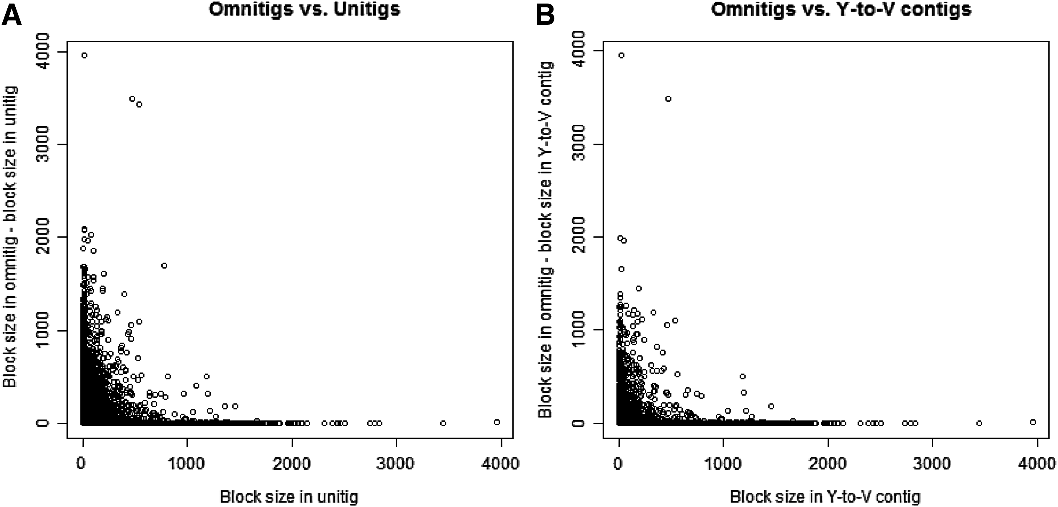
The increase in SNP block size in omnitigs compared with unitigs (A) and Y-to-V contigs (B). Each point is an SNP, and the x-value is the block size of the unitig (A) or Y-to-V contig (B) covering it. The y-value is the increase in the block size, when compared with omnitigs. Note that the y-axis does not represent the block size, but a difference of block sizes.

We also compared omnitigs with Y-to-V contigs. Y-to-V contigs have been proposed in the literature (Medvedev et al., 2007; Jackson, 2009; Kingsford et al., 2010), but, to the best of our knowledge, there has not been a quantitative study comparing their merits against other contig assembly algorithms. Omnitigs also provide more SNP context than Y-to-V contigs, with ∼266,000 SNPs having an increase in block size (Fig. 6B). Omnitigs are only marginally better than Y-to-V contigs in terms of average contiguity (Table 1). Our results suggest that, although not as beneficial as omnitigs, Y-to-V contigs may nevertheless provide a better alternative to unitigs that is faster than the omnitig algorithm.

Table 1 also shows the wall clock running times of our algorithms. The experiments were run on a node with two Xeon 2.53 GHz CPUs. We parallelized the omnitig algorithm so that it utilized all eight available cores. We observe negligible running times for all algorithms on E. coli. On chr10, the running time of the omnitig algorithm is significantly longer (by 18 mins) than the unitig or Y-to-V algorithm, although it would still not form a bottleneck in an assembly pipeline. The memory usage did not exceed 1 GB at any point, although we believe it can be significantly reduced with a more careful implementation.

9. Conclusion

There are two natural directions for future work: practical and theoretical. In the practical direction, the omnitig algorithm should be extended to handle the complexities of real data such as sequencing errors, imperfect coverage, linear genomes, and double-strandedness. This is a nontrivial task that is outside the scope of the current study, but it will be important in facilitating the application to genome analysis and assembly. In the theoretical direction, we believe that omnitigs exhibit more structure that can be exploited in a faster algorithm for finding all maximal omnitigs. We are also currently studying the graph model in which a genomic reconstruction is any collection of circular walks that together cover all nodes/edges of the graph (as in metagenomic sequencing of bacteria). We are also studying the class of genome graphs admitting a single safe walk covering all of their nodes or edges, question related to those about unique reconstructions.

Footnotes

Acknowledgments

We would like to thank Daniel Lokshtanov for initial discussions, Rayan Chikhi for feedback on the article, and Nidia Obscura Acosta for very helpful discussion on the article. This work was supported, in part, by NSF awards DBI-1356529, IIS-1453527, and IIS-1421908 to P.M. and by Academy of Finland grant 274977 to A.I.T.

Author Disclosure Statement

No competing financial interests exist.

References

Bankevich

, Nurk

, Antipov

, et al. 2012. SPAdes: A new genome assembly algorithm and its applications to single-cell sequencing. J. Comput. Biol., 19, 455–477.

Boetzer

, Henkel

C.V.

, Jansen

H.J.

, et al. 2011. Scaffolding pre-assembled contigs using SSPACE. Bioinformatics, 27, 578–579.

Boetzer

, and Pirovano

2012. Toward almost closed genomes with gapfiller. Genome Biol. 13, 1–9.

Boisvert

, Laviolette

, and Corbeil

2010. Ray: Simultaneous assembly of reads from a mix of high-throughput sequencing technologies. J. Comput. Biol., 17, 1519–1533.

Bresler

, Bresler

, and Tse

2013. Optimal assembly for high throughput shotgun sequencing. BMC Bioinformatics, 14, S18.

Chikhi

, Limasset

, Jackman

, et al. 2014. On the representation of de bruijn graphs, 35–55. In Research in Computational Molecular Biology. Springer.

Chikhi

, and Rizk

2012. Space-efficient and exact de Bruijn graph representation based on a Bloom filter, 236–248. In WABI, volume 7534 of Lecture Notes in Computer Science. Springer.

Guénoche

1992. Can we recover a sequence, just knowing all its subsequences of given length?. Comput. Appl. Biosci., 8, 569–574.

Haussler

, O'Brien

S.J.

, Ryder

O.A.

, et al. 2008. Genome 10K: A proposal to obtain whole-genome sequence for 10,000 vertebrate species. J. Hered., 100, 659–674.

10.

Idury

R.M.

, and Waterman

M.S.

1995. A new algorithm for DNA sequence assembly. J. Comput. Biol., 2, 291–306.

11.

Jackson

B.G.

2009. Parallel methods for short read assembly. Ph.D. thesis, Iowa State University.

12.

Kapun

, and Tsarev

2013a. De Bruijn superwalk with multiplicities problem is NP-hard. BMC Bioinform. 14, S7.

13.

Kapun

, and Tsarev

2013b. On NP-hardness of the paired de Bruijn sound cycle problem, 59–69. In Algorithms in Bioinformatics. Springer.

14.

Kececioglu

J.D.

1992. Exact and approximation algorithms for DNA sequence reconstruction. Ph.D. thesis, University of Arizona, Tucson, AZ, USA.

15.

Kececioglu

J.D.

, and Myers

E.W.

1995. Combinatiorial algorithms for DNA sequence assembly. Algorithmica, 13, 7–51.

16.

Kingsford

, Schatz

M.C.

, and Pop

2010. Assembly complexity of prokaryotic genomes using short reads. BMC Bioinformatics, 11, 21.

17.

Lam

, Khalak

, and Tse

2014. Near-optimal assembly for shotgun sequencing with noisy reads. BMC Bioinformatics, 15, S4.

18.

Lander

E.S.

, and Waterman

M.S.

1988. Genomic mapping by fingerprinting random clones: A mathematical analysis. Genomics, 2, 231–239.

19.

Luo

, Liu

, Xie

, et al. 2012. Soapdenovo2: An empirically improved memory-efficient short-read de novo assembler. GigaScience, 1, 18.

20.

Lysov

IuP

, Florent'ev

V.L.

, Khorlin

A.A.

, et al. 1988. Determination of the nucleotide sequence of DNA using hybridization with oligonucleotides. A new method. Dokl. Akad. Nauk SSSR, 303, 1508–1511.

21.

Medvedev

, and Brudno

2009. Maximum likelihood genome assembly. J. Comput. Biol., 16, 1101–1116.

22.

Medvedev

, Georgiou

, Myers

, et al. 2007. Computability of models for sequence assembly, 289–301. In WABI. Springer LNCS, pg. 289.

23.

Medvedev

, Pham

, Chaisson

, et al. 2011. Paired de Bruijn graphs: A novel approach for incorporating mate pair information into genome assemblers. J. Comput. Biol., 18, 1625–1634.

24.

Miller

J.R.

, Koren

, and Sutton

2010. Assembly algorithms for next-generation sequencing data. Genomics, 95, 315–327.

25.

Motahari

A.S.

, Bresler

, and Tse

D.N.C.

2013. Information theory of DNA shotgun sequencing. IEEE Trans. Inform. Theory, 59, 6273–6289.

26.

Myers

E.W.

2005. The fragment assembly string graph, 85. In ECCB/JBI. Springer LNCS 85.

27.

Nagarajan

, and Pop

2009. Parametric complexity of sequence assembly: Theory and applications to next generation sequencing. J. Comput. Biol., 16, 897–908.

28.

Nagarajan

, and Pop

2013. Sequence assembly demystified. Nat. Rev. Genet., 14, 157–167.

29.

Narzisi

, Mishra

, and Schatz

M.C.

2014. On algorithmic complexity of biomolecular sequence assembly problem, 183–195. In Algorithms for Computational Biology. Springer.

30.

Peltola

, Söderlund

, Tarhio

, et al. 1983. Algorithms for some string matching problems arising in molecular genetics, 59–64. In IFIP Congress.

31.

Pevzner

P.A.

1989. L-Tuple DNA sequencing: Computer analysis. J. Biomol. Struct. Dyn., 7, 63–73.

32.

Pevzner

P.A.

, Tang

, and Waterman

M.S.

2001. An Eulerian path approach to DNA fragment assembly. Proc. Natl. Acad. Sci. U.S.A., 98, 9748–9753.

33.

Rubinov

A.R.

, and Gelfand

M.S.

1995. Reconstruction of a string from substring precedence data. J. Comput. Biol., 2, 371–381.

34.

Sahlin

, Vezzi

, Nystedt

, et al. 2014. BESST-efficient scaffolding of large fragmented assemblies. BMC Bioinformatics, 15, 281.

35.

Salmela

, Sahlin

, Mäkinen

, et al. 2015. Gap filling as exact path length problem, 281–292. In Research in Computational Molecular Biology. Springer.

36.

Salzberg

S.L.

, Phillippy

A.M.

, Zimin

, et al. 2011. GAGE: A critical evaluation of genome assemblies and assembly algorithms. Genome Res. 22, 557–567.

37.

Simpson

J.T.

, and Durbin

2010. Efficient construction of an assembly string graph using the FM-index. Bioinformatics, 26, i367–i373.

38.

Simpson

J.T.

, and Durbin

2012. Efficient de novo assembly of large genomes using compressed data structures. Genome Res. 22, 549–556.

39.

Uricaru

, Rizk

, Lacroix

, et al. 2015. Reference-free detection of isolated SNPs. Nucleic Acids Res. 43, e11.

40.

Vyahhi

, Pyshkin

, Pham

, et al. 2012. From de Bruijn graphs to rectangle graphs for genome assembly, 249–261. In Algorithms in Bioinformatics. Springer.

41.

Waterman

M.S.

1995. Introduction to Computational Biology: Maps, Sequences and Genomes. CRC Press, New York.

42.

Zerbino

D.R.

, and Birney

2008. Velvet: Algorithms for de novo short read assembly using de Bruijn graphs. Genome Res. 18, 821–829.